Abstract
The oil and gas (O&G) industry is now as focused on minimizing costs and maximizing efficiency just as much as maximizing production. Operators are looking for new and cost-effective ways to add profitable assets to their portfolio. One such way is to re-fracture existing wells. There is evidence that these wells can be very productive in the Bakken. However, because of factors such as depletion and aging wellbore material, re-fracturing wells can be a difficult process to implement successfully and often have binding constraints on surface treating pressure (STP). This study attempts to quantify the effects that completion parameters have on re-fracturing treatment implementation by constructing dynamic fixed effects (FE) multivariate regression models. These models are not generally used in O&G and are more commonly used in economics and policy analysis. However, given that both economics and O&G deal with large amounts of uncertainty for each individual person and well, respectively, these models provide a much simpler approach to handle the uncertainty. These models also attempt to account for stress shadow effects from subsequent stages on treatment. The FE model has the advantage of treating a compilation of well treatment data as panel data and differencing out any unobservable fixed parameters. To the authors’ knowledge, this is the first study using dynamic FE models to estimate temporal stress shadow effects from one stage to the next. These models may then be thought of as estimating the boundary effects from stress shadows, which will affect treatment implementation. The novelty lies in estimating these effects, while accounting for fixed within-well variation, using simpler models than those usually found in industry. We stress that the simplicity of these models is a feature, not a bug. This study found that previous stage average STP, acid volume pumped, and perforation standoff were all statistically significant predictors of average STP with a strong temporal dependence of average STP on subsequent stages after accounting for fixed wellbore and geologic parameters. The models in this study also predict a positive marginal effect from acid volume average STP, which may seem counterintuitive, but is also backed by a previous study.
1. Introduction
Many companies are now focused on minimizing costs as much as maximizing production [1]. This pivot along with overleveraging and persistent low prices in the market have forced many operators to shift their focus towards re-developing existing assets instead of focusing on new drills and initial hydraulic fracturing (HF) stimulation [2]. Re-fractured wells may become economic due to insufficient initial stimulation [2]. Rignol and Bui (2020) estimate production from re-fractured wells to be as high as 92% of initial production in the Bakken [2]. Figure 1 shows the production gains specific to the Bakken after analyzing re-fracturing data captured from FracFocus [3]. Shammam et al. (2021) estimate production gains as high as 160% of original production in the Bakken, conditioned on proper well selection. These studies show that there is opportunity in the Bakken for operators to add economic wells to their portfolio without incurring the cost of new drills.
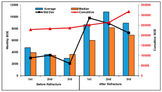
Figure 1.
Expected production gains in Bakken after re-fracturing treatment [3].
New knowledge and methods are necessary for the development of unconventional reservoirs [4]; however, until recently, no approach encompassed engineering fundamentals and data mining techniques to optimize operations with production maximization as an objective function [4]. Thus, there has been an increase in the utilization of field treatment, or time series, data and machine learning (ML) models to optimize operations. These ML models attempt to find trends and patterns in data that are used to make data-driven decisions [5] and improve well economics. Ramirez and Iriarte (2019) used field treatment data and logistic regression algorithms to predict HF stage start and end times to reduce redundant work for petroleum engineers. Ramirez and Iriarte (2019 Part II) also used an Artificial Neural Network (ANN) and field treatment data to predict Instantaneous Shut In Pressures (ISIP) which are useful in a multitude of petroleum engineering applications [6]. More recently, Ramirez and Iriarte (2021) used ML techniques to isolate time-series treatment data prior to sand entering the formation and predict breakdown pressures [7].
Expected production from re-fractured wells hinges mostly on well selection [2]. Mohaghegh et al. (2017) developed “Shale Analytics” as a self-contained process utilizing ML to optimize well spacing, predict the best candidates for re-fracturing, and construct production decline curves [8]. Other re-fracturing candidate selection algorithms were developed by Mohaghegh (2016). Mohaghegh (2016) concluded that the HF job that created the largest fracture network that maximizes O&G production is optimal, conditioned on trade-offs with costs [9]. This type of process will become increasingly important for re-fracs as well as mature plays experiencing infill drilling and encountering possible parent–child well interactions since the impact depends not only on the age of the parent well, but also on well spacing [10]. The optimization between cost and expected production is crucial for re-fracturing economics due to a high level of uncertainty [3]. Candidate selection is outside the scope of this study, and it is assumed that the best candidates were selected for re-fracturing.
The re-fracturing process is more complex than the initial HF treatment due to factors including permeability decrease from pore pressure depletion, local stress changes due to depletion, clogged perforations from production, geomechanical property changes, and fracture conductivity [11]. HF treatments with multiple stages and differing clusters leads to competition amongst different propagating fractures [12]. Wu and Olsen (2015) derived a unique fracture propagation method that incorporates propagation of closely spaced fractures, which will be affected by stress shadow effects. This also provides a physics-based model that produces realistic fracture geometries that are representative of results observed in the lab [13]. When multiple fractures are growing close to each other, the stress fields created around each fracture must be evaluated as these will affect fracture growth and treatment pressures [1]. Stress shadow factors will then affect production. This effect on production is also observed in parent–child well interactions and are probably closely related. Sakhardande and Devegowda (2021) used a covariate, causal approach to characterizing parent–child well interactions an developed an optimal well spacing method to avoid production degradation [14]. Just as parent–child well interactions may adversely affect production, fracture propagation interference within each zone will also hinder production through inefficient stimulation. This interference will result in stress shadow effects on the interior perforations resulting in more fluid, and therefore proppant, to the bookend fractures [15]. These fractures on the bookends of the stage will behave as individual fractures, regardless of the number of competing fractures between the two [1]. Poro-elastic effects also alter the net vertical stress along the wellbore [1], further complicating stress shadow estimations. Siddhamshetty, Wu, and Sang-Il Kwon (2018) constructed a novel model order reduction technique accounting for friction along the wellbore and perforations and then incorporated this into a reduced order model (ROM) that accounts for the friction drop along the fracture due to induced stress shadow effects. This was then used to optimize pump rate in combination with perforation design to achieve a limited entry design that achieves uniform fracture growth within a stage [15]. Siddhamshetty, Wu, and Sang-Il Kwon (2019) followed this study by then accounting for the additional compressive stresses on interior perforations added by stress shadow effects and proppant transport within a fracture. Combining this with their previous study allowed for the design of a pumping schedule by utilizing a ROM [16].
Stress shadow effects may be even more significant in re-fracturing treatments since decreases in pore pressure from production can lead to redistributing stresses or even reversal of principle stress in regions around fractures created during initial stimulation [17]. The types of initial completion methods vary depending on how old the well is, the prices at the time of drilling and stimulation, and the hydraulic fracturing (HF) fluid design at the time based on the understanding of the reservoir. These initial, and constant, factors along with any associated wellbore degradation may have significant effects on treatment implementation.
Kroschel, Rabiei, and Rasouli (2022) created a dynamic multivariate regression model to investigate the temporal dependence of average surface treating pressure (STP) on subsequent stages for re-fractured wells. The authors found that the distance between stages, presence of a 3.5 inches liner, average pump rate, and acid volume were all statistical predictors of average STP at the 95% level. The authors also found that the average STP from the previous stage was a statistically significant predictor of average STP at the 99% level. The estimated marginal effects of an increase in the previous stage average STP was 0.713 [18]. This pressure translation from one stage to the next may be caused by significant stress shadow effects due to depletion and possible stress reversal. However, these may also be due to things like faulty packers and cement due to aging wellbores. Therefore, it is necessary to try and control for these unobservable factors using more advanced multivariate regression models [18].
The purpose of this study is to build off the work of Kroschel, Rabiei, and Rasouli (2022) and augment the work of Siddhamshetty, Wu, and Sang-Il Kwon (2018) by investigating how stress shadow and other fixed factors in HF treatments affect the boundary conditions from one stage to another. By using the average STP of previous treatments and using panel data, we attempt to estimate the temporal dependence of STP from the one stage to the next. These models will also attempt to account for the FE previously discussed (wellbore geometry, wellbore degradation, heterogeneities, etc.). To the authors’ knowledge, there is no study using post HF treatment data as a panel data set to construct dynamic FE multivariate models. There are numerous studies on stress shadow effects on fracture propagation. However, there are also very few, if any, studies investigating the effects of stress shadow on treatment implementation. This unique approach allows for presumably fixed wellbore and geological features to be accounted for when trying to diagnose complex problems that may occur during re-fracturing treatments. There also is very little literature on using econometric models such as these to characterize HF treatments using field data and, to the authors’ knowledge, not a single study using a FE dynamic panel model to describe HF treatment behavior. There is a plethora of literature in the O&G industry of increasingly complex physics-based deterministic models that seek to fully determine fracture characterization. This is impossible and leads to overfitting. Although the physics is present, we argue that more flexible, statistical models may in fact work better in highly stochastic systems such as unconventional reservoirs.
This study was conducted after exceedingly high STP caused the abandonment of the last four stages of a recently re-fractured well. It was hypothesized that factors such as stress shadow effects, stress re-orientation, or fixed wellbore properties played a causal role in the excessively high STP. Understanding what factors might be limiting treatment is necessary to engineer solutions and implement successful HF treatments as these will play a vital role in the economics of re-fractured wells.
2. Data
Panel data is data that consists of multiple observations for an individual over time [19]. For instance, data collected for an individual person over years or data collected on a single well over years. For this study, the data consists of multiple HF treatments per well combined into a single data set. Therefore, the data is cross-sectional as it consists of multiple observations for the same well over time. Data for this study was collected from four wells that have been recently re-fractured in Dunn County, North Dakota. Figure 2 shows the location of the field in the larger context of North Dakota [20]. Individual well names and unique identifiers were not permitted to be included.
Figure 3 shows the data set as cross-sectional, separating out the groups by well with associated trendlines. Although all trend in the same direction, they do not do so at the same rate and well 3 seems to be treated drastically different than the other wells in the data set. We presume these can be at least partially explained fixed differences within-well. Variables such as wellbore trajectory, percent of wellbore out of zone, formation, etc., are expected to have different effects on treatment for each well. This presumption and the graphical evidence are why it is necessary to treat panel data appropriately and highlights the fixed effects inherent within each well. Table 1 provides the summary statistics for the data set assuming the pooled model from Kroschel, Rabiei, and Rasouli (2022) for reference. Table 2 provides definitions for each variable included in the data set with corresponding units.
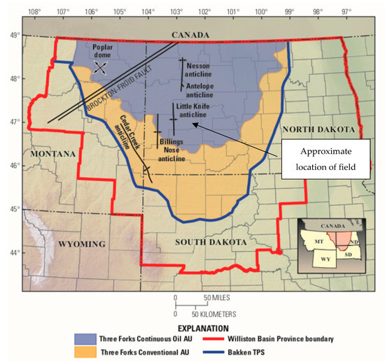
Figure 2.
Location map [20].
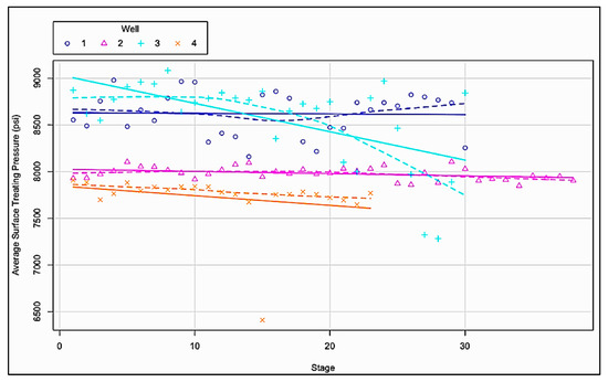
Figure 3.
Cross-sectional data set from re-fractured wells with associated trendlines highlighting the effect of different within-well characteristics.
Data for this study was not standardized. Standardizing the data would only change the interpretation of the coefficients and will have no effect on the statistical significance of variables [19]. Each unit that the dependent and independent variables are measured in is an appropriate unit for field measurement in which a marginal (per unit) increase makes sense [18]. For example, it is perfectly reasonable to increase rate, stage proppant weight, acid volume, etc., by one unit. If the model were to incorporate something like Poisson’s ratio, which is measured from 0–0.5, a one-unit increase does not make sense [18]. In this case, standardization of variables makes for valid coefficient interpretation.

Table 1.
Summary statistics for the re-fracturing data set assuming a pooled model [18].
Table 1.
Summary statistics for the re-fracturing data set assuming a pooled model [18].
| Variable | N | Mean | Std. Dev. | Min | Pctl. 25 | Pctl. 75 | Max |
|---|---|---|---|---|---|---|---|
| avg_pump_rate | 121 | 50.331 | 9.966 | 10.5 | 42.6 | 57.8 | 75.4 |
| avg_stp | 121 | 8234.355 | 465.448 | 6411 | 7903 | 8726 | 9083 |
| acid_volume | 121 | 20.711 | 30.92 | 0 | 11 | 23 | 227 |
| total_clean_volume | 121 | 3950.039 | 839.746 | 2920.091 | 3606.364 | 4024.941 | 8940.621 |
| stage_prop_weight | 121 | 220,207.884 | 37,671.035 | 25,649 | 212,565 | 218,373 | 405,515 |
| perfs | 121 | 24.165 | 1.562 | 22 | 24 | 24 | 36 |
| liner_3.5 | 121 | 0.686 | 0.466 | 0 | 0 | 1 | 1 |
| formation | 121 | 0.752 | 0.434 | 0 | 1 | 1 | 1 |
| perf_standoff | 117 | 25.573 | 4.415 | 18 | 22 | 26 | 49 |
| avg_stp_prev | 117 | 8235.778 | 467.02 | 6411 | 7907 | 8726 | 9083 |

Table 2.
Variable definitions [18].
Table 2.
Variable definitions [18].
| Variable Name | Variable Definition and Field Units |
|---|---|
| avg_pump_rate | Average total pump rate for the stage, bpm |
| avg_stp | Average surface treating pressure for the stage, psi |
| acid_volume | Total acid volume pumped for the stage, bbl |
| total_clean_volume | Total clean volume for the stage, bbl |
| stage_prop_weight | Total proppant weight pumped for the stage, lb-m |
| perfs | Total number of perforations for the stage |
| liner_3.5 | Binary variable for presence of a 3.5” liner, (1 = yes, 0 = no) |
| formation | Binary variable for formation (1 = middle Bakken, 0 = Three Forks) |
| perf_standoff | Perforation standoff for each zone, ft |
| avg_stp_prev | Previous stage average surface treating pressure used in pooled model, psi |
Figure 4, Figure 5, Figure 6, Figure 7 and Figure 8 show the individual cross plots for average STP vs. stage for each well. These highlight why treating the data as panel data is important, separating out each well instead of pooling the data together. These plots also highlight the apparent cyclical trend in average STP and provide further justification for within-well variation creating differences in treatment implementation.
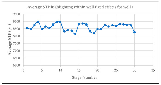
Figure 4.
Plot showing trend in average STP for well 1.
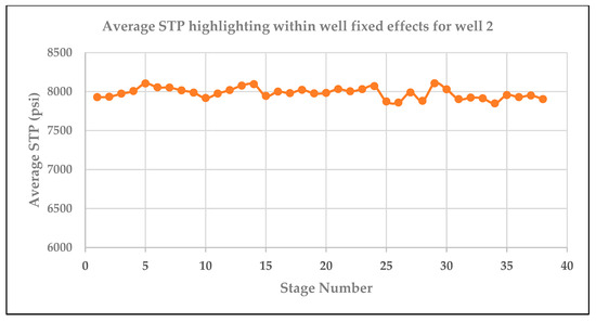
Figure 5.
Plot showing trend in average STP for well 2.
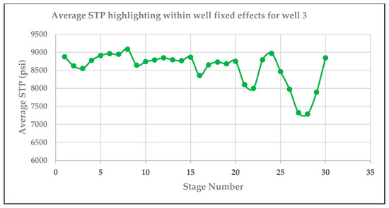
Figure 6.
Plot showing trend in average STP for well 3.
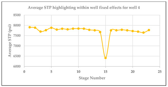
Figure 7.
Plot showing trend in average STP for well 4.
3. Materials and Methods
3.1. Multivariate Regression
Equation (1) shows the generic multivariate model that provides the basis for the models in this study [19]. Multivariate regression is an extension of bivariate regression but allows for the addition of more independent variables as controls. This approach is useful in complex systems where there is more than one causal factor affecting a dependent variable of interest.
3.2. Panel Model
However, since the data in this study has multiple observations for each well, it can be treated as “panel data” which is multiple sets of observations for given number of entities [19]. A pooled model treats all observations as independent [19]. Therefore, using a pooled data model, Equation (1), for panel data will ignore the panel nature of the data and within well variation [19]. Here is where the panel data model is introduced. Equation (2) shows the generic form of a panel data model accounting for well i over time t.
Although this model accounts for the panel nature of the data used in this study, it will be helpful to account for effects within individual wells where data was not collected, is expensive to obtain, or is outright unobservable. For instance, it is reasonable to assume that a natural fracture network that exists for a given well is unobservable in entirety. Although there may be some indications from data sources such as logs, tracers, offset well data such as fiber optic, microseismic, etc., knowing the extent of the entire natural fracture network will almost certainly not be observable for every well. Mapping the entire existing fracture network would be cost intensive. However, it is also reasonable to assume that this network will be constant prior to stimulation and constant from stage to stage during stimulation. This is where we introduce the concept of fixed effects (FE).
3.3. Fixed Effects Models
Equation (3) shows the generic form of an FE model. FE models attempt to deal with endogeneity by dividing the error term into two parts. The first part is a random error term, , and the second part is a FE term, . The FE term essentially accounts for every unobserved factor that is constant for observation of individual i.
Pulling the FE term out of the error term allows for control of anything that may be correlated with the error term and an independent variable which causes endogeneity and bias [19]. FE may be thought of as taking a long list of variables, condensing them into one variable, and then controlling for that variable [21]. This means that they control for variation between wells [21]. Things like perforation erosion, geologic properties and structure, reservoir heterogeneities, natural fracture networks, etc., will play a critical role in STP. It is presumed that these characteristics that are inherent within a well will affect treatment and may be driving the differences in trends seen in Figure 2. However, FE allows us to control for the variation that can be expected between each well.
Complex fracture geometry cannot be measured by any fracture diagnostic technique [13]. If many of these variables are presumed to be constant, they can be accounted for using an FE model without costly data collection and computationally expensive models. FE models also have the benefit of accounting for factors that are unobservable where data cannot even be collected. For example, fracture initiation depends on stress around the wellbore caused by drilling, cementing, perforating, etc. This is unobservable. However, there is no reason to assume it will change prior to treatment and could possibly remain relatively constant over the course of a wellbore. In this regard, FE models have certain advantages over deterministic physics-based models.
From the literature, there seems to be several trends that do not change significantly throughout HF treatments. Roberts, Whittaker, and Paxson (2020) conducted a study on perforation erosion that included more than 6000 clusters over 600 stages and noted the tendency for non-uniform proppant placement across a stage and a strong preference for heel-side perforation proppant placement and erosion [22]. It is also reasonable to assume that large geologic structures and wellbore characteristics will also remain constant through HF stimulation. For existing structures such as a natural fracture network, HF treatment will neither seal a pre-existing fracture nor, by definition, can it create a pre-existing fracture. Therefore, these may be thought of as constant between each well prior to and during treatment. Evidence from the literature also suggests that other geologic and geomechanical properties may be treated as constant in the middle Bakken as well. Vertical and horizontal moduli show similarity in the middle Bakken and thus indicate elastic isotropy [23,24,25]. The assumption is that any of these properties that do not vary wildly from their mean can be considered constant and captured by the FE term and thus differenced out and accounted for in the regression models using a de-meaned approach.
Production logs indicate that as many as 30% of perforations do not contribute to production due to under-stimulation from stress shadow effects [26]. Understanding and characterizing these effects, therefore, is important to increasing production and implementing effective treatments in the field. Kroschel, Rabiei, and Rasouli (2022) have already modeled the temporal dependence of average STP from one stage to the next. However, this study should give a better estimation of the temporal dependence of stress shadow effects and previous stage treatment after accounting for fixed wellbore and geologic effects, while accounting for other factors that affect treatment. Properly characterizing the temporal dependence of these effects from one stage to the next may aid engineers in effective perforation and treatment design and thus help treatment implementation in the field.
3.4. Independent Variable Selection
The independent variables were selected using domain knowledge and are the same variables that were included in the regressions constructed by Kroschel, Rabiei, and Rasouli (2022). Domain knowledge suggests that these variables are most likely to affect average STP. The results from the FE models constructed in this study will differ as any constant term will be differenced out. Therefore, the presence of a 3.5” liner, the formation, and the constant term will not appear in the regression results. These will not be discussed in the following section.
3.4.1. Previous Stage Average STP
This variable is meant to capture the temporal effects from stress shadows at the boundaries [18]. Stress interference of reorientation increases with the number of fractures created and depends on the sequence of fracturing as well [27]. Net pressure and stress contrast both also increase substantially with the number of sequential fractures and decreased fracture spacing [27]. This study will not focus on interference between fractures in the interior perforations. We instead try to measure the temporal effect of stress shadows between zones [18].
3.4.2. Perforation Standoff
Induced stress shadow from previous stages on subsequent stages has effects that extend beyond the top perforation of one stage and may thus change the fracture initiation at the bottom perforation for the next stage [1]. Therefore, the standoff (distance) between the top perforation for one stage and the bottom perforation for the next stage may affect average STP through stress shadow effects [18]. Figure 8 is a schematic of the perforation standoff in the wellbore [18].

Figure 8.
Perforation standoff between the top perforation of the previous stage and the bottom perforation of the subsequent stage [18].
3.4.3. Stage Proppant Weight
Proppant amount is an important design parameter in re-fracturing design [11]. The stage proppant weight placed during a stage affects bottom hole treating pressure by increasing the hydrostatic pressure, and therefore, negatively affects the STP [18]. The amount of proppant pumped may also affect STP from hole erosion and rounding [28].
3.4.4. Total Clean Volume
It is reasonable to assume that stage treatment size will affect the average STP. Total clean volume pumped should be an indication of treatment size. The hypothesis is that higher total clean volumes will increase average STP [18]. Fluid intensity is also more effective than proppant intensity overall at reducing diminishing effects of production [29]. This indicates that fluid intensity may have positive effects on STP. Thus, we would expect to see a positive effect from total clean volume on average STP.
3.4.5. Number of Perforations
Perforations form the conduit from wellbore to formation from which fractures will initiate and treatment will be delivered through [18]. Although only a limited number of perforations may preferentially take fluid and propagate fractures, usually the toe and heel fractures [27], it is still necessary to have a certain number of perforations above the number of fractures for pressure relief during treatment.
3.4.6. Average Pump Rate
Increases in pump rate create more friction along the wellbore and fracture. The average pump rate will most likely influence treatment costs as service companies generally charge for pump time [18]. Therefore, longer pump times will increase treatment costs which can be critical in re-fractured well economics. The assumption is that an increase in average pump rate will increase the average surface treating pressure [18].
3.4.7. Acid Volume Pumped
Acid cleans up any near wellbore damage caused by perforating and cement [18]. It can also affect average STP if the formation is carbonate. The assumption is that an increase in acid volume will decrease the average surface treating pressure [18].
4. Results
4.1. Initial Results
The results from the FE and dynamic FE models are shown in Table 3. It is important to note that any constant term was differenced out of the regression. Therefore, the constant , the presence of a 3.5″ liner, and the formation are no longer in the regression results. These along with any other unobservable fixed effect captured by the variable are now accounted for in the regression results. We see that there is still a statistically significant temporal dependence on average STP from stage to stage, although the coefficient estimate of 0.537 is smaller than that estimated from Kroschel, Rabiei, and Rasouli (2022).

Table 3.
Results from FE and dynamic FE models using the stargazer package from R [30].
The results from the models closely match those from Kroschel, Rabiei, and Rasouli (2022). However, the coefficient estimate for previous average STP is significantly lower. Model 2 estimates a temporal effect of 0.537 that is statistically significant. Perforation standoff is also positive and statistically significant which matches model estimates from Kroschel, Rabiei, and Rasouli (2022) but is counterintuitive.
One interesting note is that the marginal effects from volume of acid pumped is positive and statistically significant which also matches Kroschel, Rabiei, and Rasouli (2022). Reasons for this will be explored in the next section.
We can also perform an F-test using under the null hypothesis H0: α1 = α2 = … = αi = 0 to see if at least one of the fixed effects are non-zero (Baily, 2017). This will compare the models in this study and the pooled model from Kroschel, Rabiei, and Rasouli (2022). Table 4 shows the model results from this study as well as the results from the pooled model in Kroschel, Rabiei, and Rasouli (2022).

Table 4.
Model summaries from panel linear (FE) models and pooled models from Kroschel, Rabiei, and Rasouli (2022) using the stargazer package from R [30].
Using R and the pFtest() package, and using the above pooled and FE models, the F-statistic is 11.318 with a p-value of 0.00107 under the null hypothesis that fixed effects are zero and the alternative hypothesis that there are significant effects. Using the qf() function in R, the critical F value is 3.931. Since the F-statistic is greater than the critical value (11.318 > 3.931), we can reject the null hypothesis that at least one of the FE is 0.
Figure 9 shows the regression results with associated statistical significance. Blue indicates an estimated positive marginal effect and red indicates an estimated negative marginal effect on average STP. This provides a concise visual for quick reference for the results of alternating completion parameters on average STP.
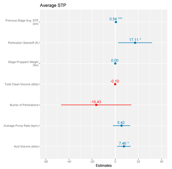
Figure 9.
Regression results showing the expected marginal effect of independent variables with associated statistical significance. Note: * p < 0.1; *** p < 0.01.
4.2. Further Model Investigation
The standard error (se) refers to accuracy of the parameter estimate which is determined by the distribution of the parameter estimate [19]. This in turn affects possible values for the estimate and statistical significance [21]. Separating the data out by well highlights an apparent cyclical trend in average STP that is different in each well. Given the nature of panel data, and the apparent trends shown in Figure 4, Figure 5, Figure 6 and Figure 7, we may want to report clustered standard errors.
We use clustered standard errors when we think there are correlations between the error terms within the group. This is common in data with multiple time periods and known as temporal autocorrelation [21]. This violates the assumption that the error term is independent and identically distributed. This assumption requires that the error term is uncorrelated with error terms for each observation (independent) and has the same distribution for each observation (independently distributed) [21]. Therefore, if the error term for one observation can predict another (as is in the case of cycles or seasonal trends), the error terms are correlated. The following plots indicate that there is some autocorrelation between stages.
Table 5 shows that the coefficient estimates have not changed; however, the statistical significance of a few variables has changed. The se for each coefficient estimate is reported in parentheses. These results indicate that previous stage average STP, perforation standoff, the number of perforations, and acid volume pumped are all statistically significant at the 99% level and the average pump rate is significant at the 95% level. Therefore, for those variables at the 99% level, we can reject the null hypothesis that the coefficient estimate is 0 with 99% confidence and we can reject the null that the coefficient estimate for average pump rate is 0 with 95% confidence. The results for each statistically coefficient estimates are discussed below.

Table 5.
Results from the dynamic FE model with clustered se using the stargazer package from R [30].
4.3. Coefficient Estimates
4.3.1. Previous Stage Average STP
The coefficient estimate for the previous stage average STP indicates that a 1 psi change in average STP for a stage is linearly associated with a temporal effect of a 0.537 psi increase in average STP for the subsequent stage. This estimate is significantly lower than estimated using the pooled model from Kroschel, Rabiei, and Rasouli (2022). This coefficient gives an estimate of the boundary effects from stress shadows as this estimates the temporal pressure translation from one stage to the subsequent stage.
4.3.2. Perforation Standoff
The coefficient estimate for perforation standoff indicates that a 1 psi change in perforation standoff between stages is linearly associated with a 17.112 psi increase in average STP for the subsequent stage. This estimate is counterintuitive, but consistent with the estimates from Kroschel, Rabiei, and Rasouli (2022). This indicates that increasing the perforation standoff between zones actually increases the average STP in expectation.
4.3.3. Number of Perforations
The coefficient estimate for number of perforations indicates that adding 1 perforation is linearly associated with a 16.432 psi decrease in average STP for the stage. This makes sense intuitively as adding entry points and conduits from wellbore to formation should yield pressure relief. This is also observed anecdotally when cleaning up a wellbore and retrieving the frac ball for the previous stage after flowing back into a well. Well cleanup is much easier when pumping across two zones as opposed to one.
4.3.4. Average Pump Rate
The coefficient estimate for average pump rate indicates that a 1 bpm change in average pump rate is linearly associated with a 5.418 psi increase in average STP for the stage. This also makes sense intuitively since increasing the rate increases friction along the wellbore and fracture.
4.3.5. Acid Volume Pumped
The coefficient estimate for acid volume pumped indicates that a 1 bbl change in acid placed in formation is linearly associated with a 7.457 psi increase in average STP for the subsequent stage. This finding is counterintuitive, but consistent with the results from Kroschel, Rabiei, and Rasouli (2022). Possible reasons are examined in the next section.
5. Discussion
The FE model in this study cannot be used for prediction since all fixed wellbore effects and intercepts were differenced from the data. This model only provides an estimation of effect sizes and would need to be augmented with a physics-based model or direct observation from fiber optics. Experiments would need to be set up in the field by design. This could be tested anecdotally, for example, by increasing the perforation standoff between zones. The hypothesis could also be tested by changing the perforation standoff halfway through well completions and constructing a difference in difference model and investigating the effects of the change in design. This will hopefully be investigated in a future study.
Haustveit, Elliot, and Roberts (2022) derived a novel solution to estimate net pressure using bottom hole pressure gauge (BHPG) data to measure poroelastic responses from stress shadows. Although the primary application from Haustveit, Elliot, and Roberts (2022) was to estimate net pressure, they observed a temporal dependence from poroelastic effects and net pressure from subsequent stages relative to a fixed BHPG at the toe of a well. They observed a diminishing temporal dependence since the measured poroelastic effect from stages 3–7 was measured relative to a BHPG fixed near stage 1 in the wellbore [31]. This makes sense intuitively as one would expect to lose serial correlation the further from the measuring device each sample was taken. Our study augments Haustveit, Elliot, and Roberts (2022) by providing an estimate of the temporal dependence on average STP from one stage to the next as opposed temporal poroelastic responses to a fixed point in the wellbore.
These models only yield insights about the fixed effects within wells contained in the dataset. Prediction would not be clear since the models are not accounting for other wells which have their own within-well variation that is not captured by the model. These models are only used as a tool to investigate the temporal dependence of average STP. More data for re-fracturing treatments is necessary to expand on this idea and provide estimates of temporal dependence that may differ by company, location, formation, etc.
It is interesting to note that the coefficient estimate for acid volume from both the FE (model 1 in Table 4) and dynamic FE model (model 2 in Table 4) is positive. This also matches the results from Kroschel, Rabiei, and Rasouli (2022) yielding strong evidence that increasing acid volume tends to increase average STP in re-fractured wells. Cross et al. (2021) hypothesized that the Bakken may experience quicker production decay from fluid and proppant intensity because the Bakken more resembles a hybrid formation instead of a true unconventional formation [29]. The same logic may apply to the effects of acid. Acid may be less effective due to things like mineralogy and formation properties. Another possibility may be that the acid is opening more interior perforations; thus, increasing overall fracture width but decreasing individual fracture width as individual fractures compete at a constant rate and pressure [32], and increasing total friction along the fracture face. There is also the possibility of faulty acid or insufficient mixing on location as the acid is delivered to the location raw and cut with water on-the-fly. One area of increasing interest is that of supramolecular complexes fracture fluids. Bhat et al. (2021) introduced a novel supramolecular-structure-based fluid that is used in alkaline conditions [33]. Assuming acid is opening interior perforations, which will increase overall width while decreasing individual width, these new fluid structures may help alleviate individual fracture width restrictions. One advantage of this fluid is that its properties are amplified in the presence of salt [33]. This may prove even more useful as produced water reuse is becoming more common in HF designs.
One possible source of endogeneity is that independent variables such as perforations and perforation standoff vary only slightly within the dataset. More data is needed with more diverse perforation stand-off, clusters, and number of perforations per cluster.
It is important to reiterate that the coefficient estimates will be biased due to the structure of the model. One way to combat this is to use what is known as an instrumental variable (IV) but these can be complicated and lead to imprecise results [19]. However, it is worth noting that the bias becomes less severe as the number of observations for each panel (in this case each well) increases. For observations over ~20, the problem of bias becomes less serious [19]. Thus, since there are more than 20 observations for each well in the data set, the bias will be accepted as tolerable.
This FE model does not specifically account for well–well interactions as this would be a different type of model. Interactions between wells that are on a single pad may also exist and were not accounted for in this study. These interactions will be investigated in a future study.
6. Conclusions
- Unobservable wellbore and geologic properties that do not vary wildly from stage to stage may be accounted for using fixed effects (FE) multivariate regression models. These models also allow for estimation of boundary effects from stress shadows from one stage to the next. These estimates may differ by formation due to inherent geologic, reservoir, and wellbore differences. However, having an estimate on the temporal dependence of pressure between stages may be an important design parameter for treatments, perforation design, and field implementation.
- After accounting for FE, previous stage average STP, perforation standoff, and acid volume pumped were the only statistically significant predictors of average STP for a re-fracturing treatment. Based on our models, a marginal increase in average STP in one stage will yield a 0.537 psi increase in the subsequent stage. This is significantly smaller than our previous estimate. This estimate of boundary conditions and temporal dependence of average STP is the novelty of this study.
- The amount of acid pumped seems to have a positive and statistically significant effect on average STP. This assertion is backed by the models constructed in this study as well as the models constructed from Kroschel, Rabiei, and Rasouli (2022). From field experience, this is often seen anecdotally, and acid is often cut out of the treatment due to little to no pressure relief. This may be due to interior perforations being opened, decreasing individual fracture width and increasing perforation friction pressure as well as friction pressure along the fracture face.
- Characterizing stage to stage interactions and how completion parameters affect treatment from stage to stage may be an important modeling parameter that can be incorporated into more complex fracture models. The models constructed in this study may be augmented with more complex fracture models and fiber optic data to verify the model predictions with fiber optic measurements.
Author Contributions
Conceptualization, J.K.; methodology, J.K.; software, J.K.; validation, J.K., M.R., and V.R.; formal analysis, J.K.; investigation, V.R.; resources, M.R.; data curation, J.K.; writing—original draft preparation, J.K.; writing—review and editing, M.R. and V.R.; visualization, M.R.; supervision, M.R.; project administration, M.R. and V.R. All authors have read and agreed to the published version of the manuscript.
Funding
This research received no external funding.
Informed Consent Statement
Not applicable.
Conflicts of Interest
The authors declare no conflict of interest.
References
- Barree, R. Potential Issues with Limited Entry Horizontal Wells. In Proceedings of the Unconventional Resources Technology Conference, Austin, TX, USA, 20–22 July 2020. URTEC-2020-1024-MS. [Google Scholar] [CrossRef]
- Rignol, V.; Bui, B. The Key Factors for Re-fracturing Success: A Simulation Study. In Proceedings of the 54th US Rock Mechanics/Geomechanics Symposium, Golden, CO, USA, 28 June–1 July 2020. [Google Scholar]
- Shammam, F.O.; Alkinani, A.; Al-Hameddi, A.T.; Dunn-Norman, S.; Al-alwani, M.A. Assesment of Production Gain From Refracturing Wells in the Major Shale Plays in the United States. In Proceedings of the 55th Annual U.S. Rock Mechanics/Geomechanics Symposium, Held Virtually. 20–23 June 2021. [Google Scholar]
- Kumar, A.; Shih, C.; Liu, G.; Holcomb, P.; Zhao, S.; Hammack, R.; Bromhal, G. Machine Learning Applications for a Qualitative Evaluation of the Fracture Network in the Wolfcamp Sahle Using Tracer and Completion Data. In Proceedings of the Unconventional Resources Technology Conference, Houston, TX, USA, 26–28 July 2021. [Google Scholar]
- Ramirez, A.; Iriarte, J. Event Recognition on Time Series Frac Data Using Machine Learning. In Proceedings of the SPE Western Regional Metting, San Jose, CA, USA, 23–26 April 2019. [Google Scholar]
- Ramirez, A.; Iriarte, J. Event Recognition on Time Series Frac Data Using Machine Learning—Part II. In Proceedings of the SPE Liquids-Rich Basins Conference-North America, Odessa, TX, USA, 7–8 November 2019. [Google Scholar]
- Ramirez, A.J.; Iriarte, J.G. Novel Application to Recognize a Breakdown Pressure Event on Time Series Frac Data vs. An Artificial Intelligence Approach. In Proceedings of the SPE Western Regional Meeting, Held Virtually. 20–22 April 2021. [Google Scholar]
- Mohaghegh, S.; Gaskari, R.; Maysami, M. Shale Analytics: Making Production and Operational Decisions Based on Facts: A Case Study in Marcellus Shale. In Proceedings of the SPE Hydraulic Fracturing Technology Conference and Exhibition, The Woodlands, TX, USA, 24–26 January 2017. SPE-184822-MS. [Google Scholar] [CrossRef] [Green Version]
- Mohaghegh, S. Fact Based Re-Frac Candidate Selection and Design in Shale—A Case Study in Application of Data Analytics. In Proceedings of the Unconventional Resources Technology Conference, San Antonio, TX, USA, 1–3 August 2016. [Google Scholar] [CrossRef] [Green Version]
- Ratcliff, D.; McClure, M.; Fowler, G.; Elliot, B.; Qualls, A. Modelling of Parent Child Well Interactions. In Proceedings of the SPE Hydraulic Fracturing Technology Conference and Exhibition, The Woodlands, TX, USA, 1–3 February 2022. [Google Scholar]
- Li, C.; Han, J.; LaFollette, R.; Kotov, S. Lessons LEarned From Refractured Wells: Using Data to Develop an Engineered Approach to Rejuvenation. In Proceedings of the SPE Hydraulic Fracturing Technology Conference, The Woodlands, TX, USA, 9–11 February 2016. [Google Scholar]
- Damjanac, B.; Maxwell, S.; Pirayehgar, A.; Torres, M. Numerical Study of Stress Shadowing Effect on Fracture Initiation and Interaction between Perforation Clusters. In Proceedings of the Unconventional Resources Technology Conference, Houston, TX, USA, 23–25 July 2018. URTEC-2901800-MA. [Google Scholar] [CrossRef]
- Wu, K.; Olson, J. Simultaneous Multifracture Treatments: Fully Coupled Fluid Flow and Fracture Mechanics for Horizontal Wells. In Proceedings of the SPE Annual Technical Conference and Exhibition, New Orleans, LA, USA, 30 September–2 October 2015. [Google Scholar]
- Sakhardande, R.; Devegowda, D. Data-Driven Causal analyses of Parent-Child Well Interactions for Well Spacing Decisions. In Proceedings of the SPE Hydraulic Fracturing Technology Conference and Exhibition, Held Virtually. 4–6 May 2021. [Google Scholar]
- Siddhamshetty, P.; Wu, K.; Sang-Il Kwon, J. Optimizatio of Simultaneously Propagating Fractures in Hydraulic Fracturing to Achieve Uniform Growth Using Data-Based Model Reduction. Chem. Eng. Res. Des. 2018, 136, 675–686. [Google Scholar] [CrossRef]
- Siddhamshetty, P.; Wu, K.; Sang-Il Kwon, J. Modeling and Control of Proppant Distribution Distribution of Multistage Hydraulic Fracturing in Horizontal Shale Wells. Ind. Eng. Chem. Res. 2019, 58, 3159–3169. [Google Scholar] [CrossRef]
- He, J.; Pei, Y.; Sepehrnoori, K. Impact of Stochastic Hydraulic Fracture Properties on Stress Reorientation in Shale Gas Reservoirs. In Proceedings of the 55th US Rock Mechanics/Geomechanics Symposium, Houston, TX, USA, 20–23 June 2021. ARMA-2021-1340. [Google Scholar]
- Kroschel, J.; Rabiei, M.; Rasouli, V. Prediction of Re-Fracturing Average Surface Treating Pressure in the Williston Basin Using Multivariate Regression. Energies 2022, 15, 2271. [Google Scholar] [CrossRef]
- Baily, M. Real Econometrics: The Right Tools to Answer Important Questions, 1st ed.; Oxford University Press: New York, NY, USA, 2017. [Google Scholar]
- Gaswirth, S.; Marra, K.; Cook, T.; Charpentier, R.; Gautier, D.; Higley, D.; Whidden, K. Assesment of Undiscovered OIl Resources in the Bakken and Three Forks Formations, Williston Basin Province, Montana, North Dakota, and South Dakota 2013. USA Geol. Surv. Fact. Sheet 2013, 3013, 4. [Google Scholar]
- Huntington-Klein, N. The Effect: An Introduction to Research Design and Causality; CRC Press: Boca Raton, FL, USA, 2022. [Google Scholar]
- Roberts, G.; Whittaker, J.; Paxson, T. Proppoant Distribution Observations from 20,000+ Perforation Measurements. In Proceedings of the SPE Hydraulic Fracturing Technology Conference and Exhibition, The Woodlands, TX, USA, 4–6 February 2020. [Google Scholar]
- Ostadhassan, M. Geomechanics and Elastic Anisotropy of the Bakken Formation, Williston Basin. Ph.D. Thesis, University of North Dakota, Grand Forks, ND, USA, 2013. [Google Scholar]
- Havens, J. Mechanical Properties of the Bakken Formation. Master’s Thesis, Colorado School of Mines, Golden, CO, USA, 2012. [Google Scholar]
- Ostadhassan, M.; Zeng, Z.; Zamiran, S. Geomechanical modeling of an anisotropic formation–Bakken case study. In Proceedings of the 46th US Rock Mechanics/Geomechanics Symposium, Chicago, IL, USA, 24–27 June 2012. [Google Scholar]
- Huang, J.; Datta-Gupta, A. Optimization of Hydraulic Fracture Development and Well Performance Using Limited Entry Perforations. In Proceedings of the SPE Oklahoma City Oil and Gas Symposium, Oklahoma City, OK, USA, 27–31 March 2017. [Google Scholar]
- Roussel, N.; Sharma, M. Optimizing Fracture Spacing and Sequencing in Horizontal-Well Fracturing. In Proceedings of the SPE International Symposium and Exhibition on Formation Damage Control, Lafayette, LA, USA, 10–12 February 2011. SPE-127986-PA. [Google Scholar] [CrossRef]
- Behrmann, A.; Nolte, K. Perforating Requirements for Fracture Stimulations. In Proceedings of the SPE International Symposium on Formation Damage Control, Lafayette, LA, USA, 18–19 February 1998. [Google Scholar] [CrossRef]
- Cross, T.; Niederhut, D.; Cui, A.; Sathaye, K.; Chaplin, J. Quantifying the Diminishing Impact of Completions Over Time Across the Bakken, Eagle Ford, and Wolfcamp Using Multi-Target Machine Learning Model and SHAP Values. In Proceedings of the Unconventional Resources Technology Conference, Houston, TX, USA, 26–28 July 2021. [Google Scholar]
- Hlavac, M. Stargazer: Well-Formatted Regression and Summary Statistic Tables. Central European Labor Studies Institute (CELSI). 2018. Available online: https://CRAN-Rproject.org/package=stargazer (accessed on 23 June 2022).
- Haustveit, K.; Elliot, B.; Roberts, J. Empirical Meets Analytical-Novel Case Study Quantifies Fracture Stress Shadowing and Net Presure Using Bottom Hole Pressure and Optical Fiber. In Proceedings of the SPE Hydraulic Fracturing Technology Conference and Exhibition, The Woodlands, TX, USA, 1–3 February 2022. [Google Scholar]
- Cleary, M.; Johnson, D.; Kogsboll, H.; Owens, K.; Perry, K.; de Pater, C.; Mauro, T. Field Implementation of Proppant Slugs to Avoid Premature, Screen-Out of Hydraulic Fractures with Adequate Proppant Concentration. In Proceedings of the Low Permeability Reservoir Symposium, Denver, CO, USA, 26–28 April 1993. SPE-25892-MS. [Google Scholar] [CrossRef]
- Bhat, B.; Lui, S.; Lin, Y.; Sentmanat, M.; Kwon, J.; Akbulut, M. Supramolecular Dynamic Binary Complexes with pH and Salt-Responsive Properties for use in Unconventional Resrvoirs. PLoS ONE 2021, 16, e0260786. [Google Scholar] [CrossRef] [PubMed]
Publisher’s Note: MDPI stays neutral with regard to jurisdictional claims in published maps and institutional affiliations. |
© 2022 by the authors. Licensee MDPI, Basel, Switzerland. This article is an open access article distributed under the terms and conditions of the Creative Commons Attribution (CC BY) license (https://creativecommons.org/licenses/by/4.0/).