
Assessing China’s Investment Risk of the Maritime Silk Road: A Model Based on Multiple Machine Learning Methods

Abstract
:1. Introduction
- As far as we know, this study is the first to use ICRG data combined with the machine learning methods to predict China’s investment risks in the Maritime Silk Road region. In the prediction process, China’s foreign investment data was used to replace the weighted risk results from ICRG data, improving the assessment results’ objectivity and effectiveness.
- Machine learning and deep learning technologies were applied to the prediction model, and multi-source information of the current year was used to predict the investment risk of China in the Maritime Silk Road region in the next year, with an accuracy rate of 86%.
2. Data
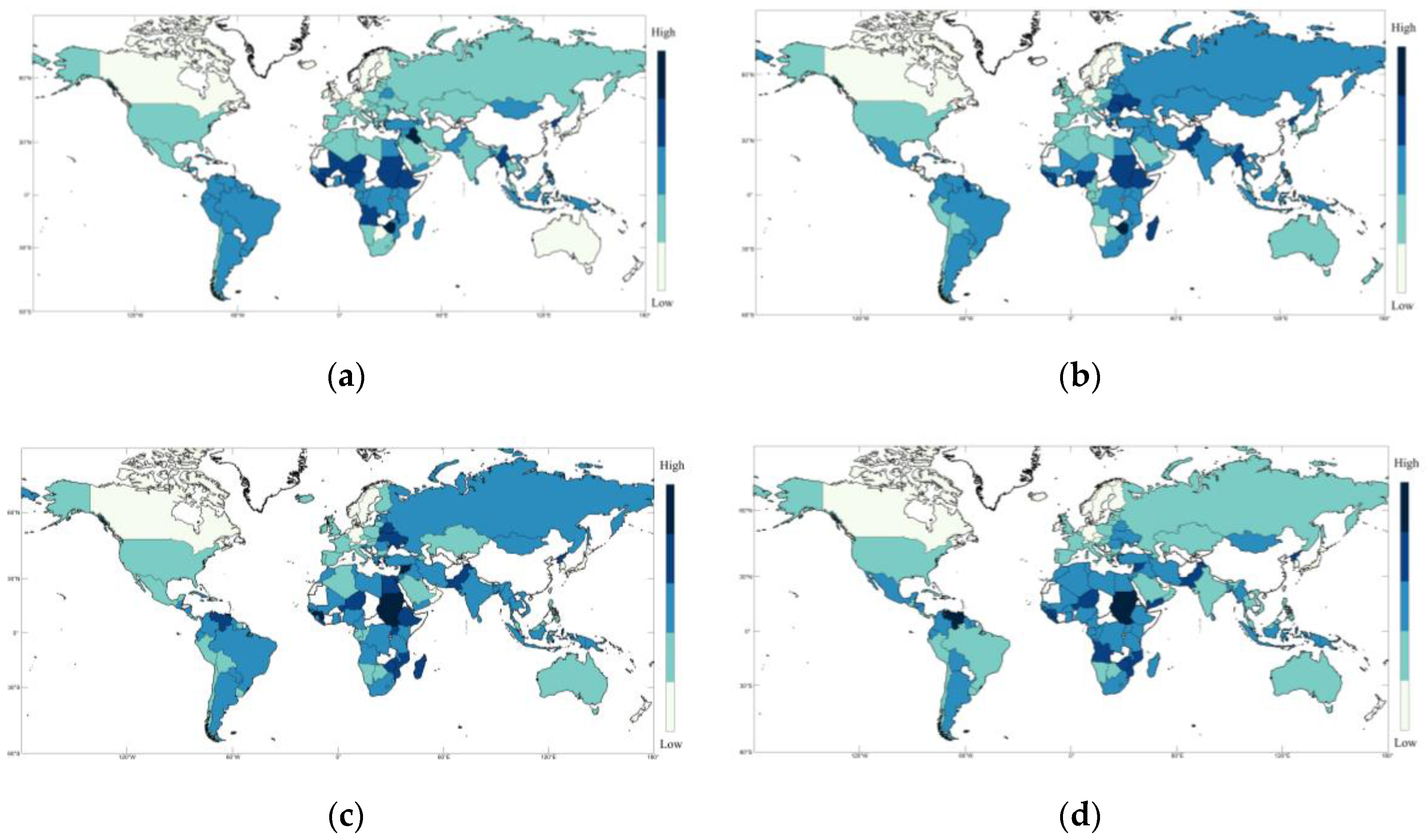
2.1. ICRG
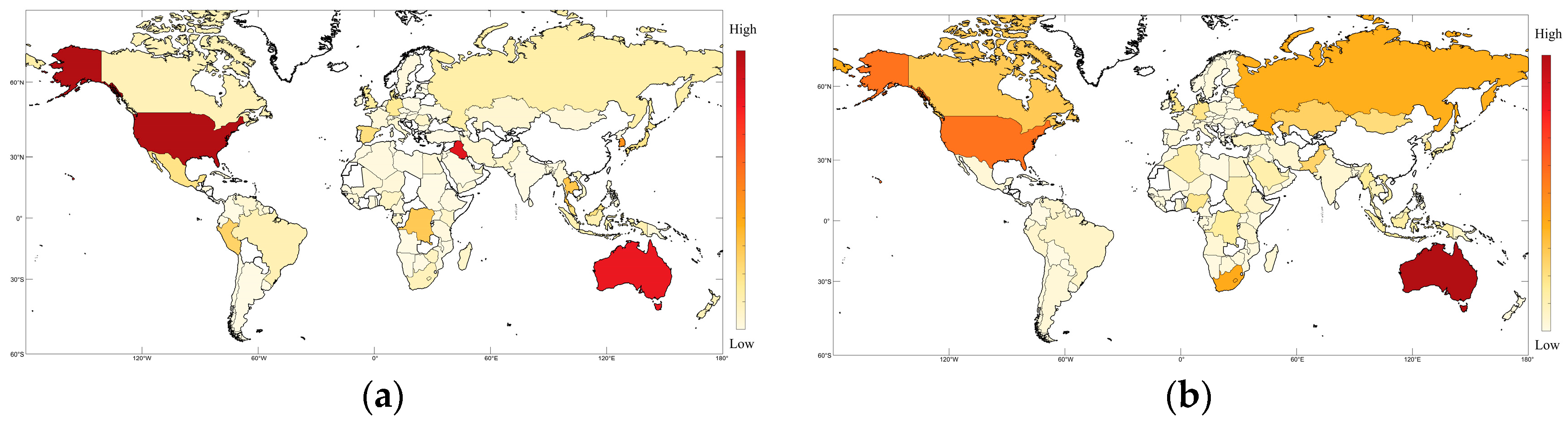
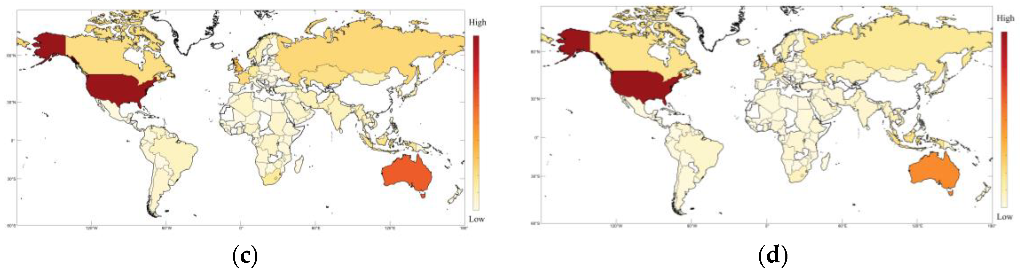
2.2. OFDI
2.3. Historical Situation Analysis
2.4. Data Preprocessing
3. Methods
3.1. Machine Learning
3.1.1. SVM
3.1.2. XGB
3.1.3. LightGBM
3.1.4. Random Forest
3.1.5. KNN
3.1.6. Logistic Regression
3.2. Deep Learning
DNN
3.3. Research Flow
3.3.1. Machine Learning
3.3.2. Deep Learning
3.4. Evaluation Indicators
4. Results and Discussion
4.1. Accuracy
4.2. Local Prediction Effect
4.3. Discussion
5. Conclusions
Author Contributions
Funding
Conflicts of Interest
References
- Hall, S.; Du Gay, P. Questions of Cultural Identity; Sage: Thousand Oaks, CA, USA, 1996. [Google Scholar]
- Schinas, O.; von Westarp, A.G. Assessing the Impact of the Maritime Silk Road. J. Ocean. Eng. Sci. 2017, 2, 186–195. [Google Scholar] [CrossRef]
- Busse, M.; Hefeker, C. Political Risk, Institutions and Foreign Direct Investment. Eur. J. Polit. Econ. 2007, 23, 397–415. [Google Scholar] [CrossRef] [Green Version]
- Zhang, X. Interpret the Legal Risk Management of Overseas Investment under the New Situation of “One Belt and One Road”. Int. Eng. Labor 2015. [Google Scholar]
- Flint, C.; Zhu, C. The Geopolitics of Connectivity, Cooperation, and Hegemonic Competition: The Belt and Road Initiative. Geoforum 2019, 99, 95–101. [Google Scholar] [CrossRef]
- Ukwueze, E.R.; Ugwu, U.C.; Okafor, O.A. Impact of Institutional Quality on Multilateral Aid in Nigeria. J. Econ. Sci. Res. 2021, 4, 3116. [Google Scholar] [CrossRef]
- Javaid, A.; Arshed, N.; Munir, M.; Zakaria, Z.A.; Alamri, F.S.; Abd El-Wahed Khalifa, H.; Hanif, U. Econometric Assessment of Institutional Quality in Mitigating Global Climate-Change Risk. Sustainability 2022, 14, 699. [Google Scholar] [CrossRef]
- Mullainathan, S.; Spiess, J. Machine Learning: An Applied Econometric Approach. J. Econ. Perspect. 2017, 31, 87–106. [Google Scholar] [CrossRef] [Green Version]
- Lecun, Y.; Bengio, Y.; Hinton, G. Deep Learning. Nature 2015, 521, 436–444. [Google Scholar] [CrossRef]
- Kamilaris, A.; Prenafeta-Boldú, F.X. Deep Learning in Agriculture: A Survey. Comput. Electron. Agric. 2018, 147, 70–90. [Google Scholar] [CrossRef] [Green Version]
- Brown, C.L.; Cavusgil, S.T.; Lord, A.W. Country-Risk Measurement and Analysis: A New Conceptualization and Managerial Tool. Int. Bus. Rev. 2015, 24, 246–265. [Google Scholar] [CrossRef]
- Gezikol, B.; Tunahan, H. The Econometric Analysis of the Relationship between Perceived Corruption, Foreign Trade and Foreign Direct Investment in the Context of International Indices. Alphanumeric J. 2018, 6, 117. [Google Scholar] [CrossRef] [Green Version]
- Rawson, A.; Brito, M. A Survey of the Opportunities and Challenges of Supervised Machine Learning in Maritime Risk Analysis. Transp. Rev. 2022, 1–23, in press. [Google Scholar] [CrossRef]
- Xiong, Y.; Zhu, M.; Li, Y.; Huang, K.; Chen, Y.; Liao, J. Recognition of Geothermal Surface Manifestations: A Comparison of Machine Learning and Deep Learning. Energies 2022, 15, 2913. [Google Scholar] [CrossRef]
- Akyuz, E.; Cicek, K.; Celik, M. A Comparative Research of Machine Learning Impact to Future of Maritime Transportation. Procedia Comput. Sci. 2019, 158, 275–280. [Google Scholar] [CrossRef]
- Pisner, D.A.; Schnyer, D.M. Support Vector Machine. In Machine Learning: Methods and Applications to Brain Disorders; Mechelli, A., Vieira, S., Eds.; Elsevier: Amsterdam, The Netherlands, 2019; pp. 101–121. [Google Scholar] [CrossRef]
- Christopher, J.C. Burges A Tutorial on Support Vector Machines for Pattern Recognition. Data Min. Knowl. Discov. 1998, 2, 121–167. [Google Scholar]
- Ali, W.; Tian, W.; Din, S.U.; Iradukunda, D.; Khan, A.A. Classical and Modern Face Recognition Approaches: A Complete Review. Multimed. Tools Appl. 2021, 80, 4825–4880. [Google Scholar] [CrossRef]
- Pan, B. Application of XGBoost Algorithm in Hourly PM2.5 Concentration Prediction. IOP Conf. Ser. Earth Environ. Sci. 2018, 113, 12127. [Google Scholar] [CrossRef] [Green Version]
- Nobre, J.; Neves, R.F. Combining Principal Component Analysis, Discrete Wavelet Transform and XGBoost to Trade in the Financial Markets. Expert Syst. Appl. 2019, 125, 181–194. [Google Scholar] [CrossRef]
- Gumus, M.; Kiran, M.S. Crude Oil Price Forecasting Using XGBoost. In Proceedings of the 2017 International Conference on Computer Science and Engineering (UBMK), Antalya, Turkey, 5–8 October 2017; pp. 1100–1103. [Google Scholar] [CrossRef]
- Zhang, D.; Qian, L.; Mao, B.; Huang, C.; Huang, B.; Si, Y. A Data-Driven Design for Fault Detection of Wind Turbines Using Random Forests and XGboost. IEEE Access 2018, 6, 21020–21031. [Google Scholar] [CrossRef]
- Chen, T.; Guestrin, C. XGBoost: A Scalable Tree Boosting System. In Proceedings of the 22nd ACM SIGKDD International Conference, San Francisco, CA, USA, 13–17 August 2016. [Google Scholar]
- Shi, X.; Wong, Y.D.; Li, M.Z.F.; Palanisamy, C.; Chai, C. A Feature Learning Approach Based on XGBoost for Driving Assessment and Risk Prediction. Accid. Anal. Prev. 2019, 129, 170–179. [Google Scholar] [CrossRef]
- Ren, X.; Guo, H.; Li, S.; Wang, S. A Novel Image Classi Fi Cation Method with CNN-XGBoost Model. In Proceedings of the 16th International Workshop, IWDW 2017, Magdeburg, Germany, 23–25 August 2017; pp. 378–390. [Google Scholar] [CrossRef]
- Ogunleye, A.; Wang, Q.G. XGBoost Model for Chronic Kidney Disease Diagnosis. IEEE ACM Trans. Comput. Biol. Bioinform. 2020, 17, 2131–2140. [Google Scholar] [CrossRef] [PubMed]
- Fan, J.; Wang, X.; Wu, L.; Zhou, H.; Zhang, F.; Yu, X.; Lu, X.; Xiang, Y. Comparison of Support Vector Machine and Extreme Gradient Boosting for Predicting Daily Global Solar Radiation Using Temperature and Precipitation in Humid Subtropical Climates: A Case Study in China. Energy Convers. Manag. 2018, 164, 102–111. [Google Scholar] [CrossRef]
- Ke, G.; Meng, Q.; Finley, T.; Wang, T.; Chen, W.; Ma, W.; Ye, Q.; Liu, T.Y. LightGBM: A Highly Efficient Gradient Boosting Decision Tree. In Proceedings of the 31st Conference on Neural Information Processing Systems (NIPS 2017), Long Beach, CA, USA, 4–9 December 2017; pp. 3147–3155. [Google Scholar]
- Tang, M.; Zhao, Q.; Ding, S.X.; Wu, H.; Li, L.; Long, W.; Huang, B. An Improved LightGBM Algorithm for Online Fault Detection of Wind Turbine Gearboxes. Energies 2020, 13, 807. [Google Scholar] [CrossRef] [Green Version]
- Wang, D.; Zhang, Y.; Zhao, Y. LightGBM: An Effective MiRNA Classification Method in Breast Cancer Patients. In Proceedings of the 2017 International Conference on Computational Biology and Bioinformatics, Newark, NJ, USA, 18–20 October 2017; pp. 7–11. [Google Scholar] [CrossRef]
- Javier, P.; Camino, G.; Javier, M. Electricity Price Forecasting with Dynamic Trees: A Benchmark Against the Random Forest Approach. Energies 2018, 11, 1588. [Google Scholar]
- Breiman, L. Random Forests. Mach. Learn. 2001, 45, 5–32. [Google Scholar] [CrossRef] [Green Version]
- Liaw, A.; Wiener, M. Classification and Regression by Random Forest. R News 2002, 2/3, 18–22. [Google Scholar]
- Karballaeezadeh, N.; Ghasemzadeh Tehrani, H.; Mohammadzadeh Shadmehri, D.; Shamshirband, S. Estimation of Flexible Pavement Structural Capacity Using Machine Learning Techniques. Front. Struct. Civ. Eng. 2020, 14, 1083–1096. [Google Scholar] [CrossRef]
- Guo, G.; Wang, H.; Bell, D.; Bi, Y.; Greer, K. KNN Model-Based Approach in Classification. In Proceedings of the On The Move to Meaningful Internet Systems 2003: CoopIS, DOA, and ODBASE, Sicily, Italy, 3–7 November 2003; pp. 986–996. [Google Scholar] [CrossRef]
- Zhang, M.L.; Zhou, Z.H. ML-KNN: A Lazy Learning Approach to Multi-Label Learning. Pattern Recognit. 2007, 40, 2038–2048. [Google Scholar] [CrossRef] [Green Version]
- Zhang, S.; Li, X.; Zong, M.; Zhu, X.; Wang, R. Efficient KNN Classification with Different Numbers of Nearest Neighbors. IEEE Trans. Neural Netw. Learn. Syst. 2018, 29, 1774–1785. [Google Scholar] [CrossRef]
- Weinberger, K.Q.; Saul, L.K. Distance Metric Learning for Large Margin Nearest Neighbor Classification. J. Mach. Learn. Res. 2009, 10, 207–244. [Google Scholar]
- Zhang, H.; Berg, A.; Maire, M.; Malik, J. SVM-KNN: Discriminative Nearest Neighbor Classification for Visual Category Recognition. In Proceedings of the 2006 IEEE Computer Society Conference on Computer Vision and Pattern Recognition (CVPR’06), New York, NY, USA, 17–22 June 2006; pp. 2126–2136. [Google Scholar]
- Trstenjak, B.; Mikac, S.; Donko, D. KNN with TF-IDF Based Framework for Text Categorization. Procedia Eng. 2014, 69, 1356–1364. [Google Scholar] [CrossRef] [Green Version]
- Pratama, B.Y.; Sarno, R. Personality Classification Based on Twitter Text Using Naive Bayes, KNN and SVM. In Proceedings of the 2015 International Conference on Data and Software Engineering (ICoDSE), Yogyakarta, Indonesia, 25–26 November 2016; pp. 170–174. [Google Scholar] [CrossRef]
- Nguyen, A.; Yosinski, J.; Clune, J. Deep Neural Networks Are Easily Fooled: High Confidence Predictions for Unrecognizable Images. In Proceedings of the 2015 IEEE Conference on Computer Vision and Pattern Recognition (CVPR), Boston, MA, USA, 7–12 June 2015. [Google Scholar]
- Moosavi-Dezfooli, S.M.; Fawzi, A.; Frossard, P. DeepFool: A Simple and Accurate Method to Fool Deep Neural Networks. In Proceedings of the 2016 IEEE Conference on Computer Vision and Pattern Recognition (CVPR), Las Vegas, NV, USA, 27–30 June 2016. [Google Scholar]
- Seltzer, M.L.; Dong, Y.; Wang, Y. An Investigation of Deep Neural Networks for Noise Robust Speech Recognition. In Proceedings of the IEEE International Conference on Acoustics, Speech and Signal Processing, Vancouver, BC, Canada, 26–31 May 2013. [Google Scholar]
- Lee, S.; Cho, S.; Kim, S.H.; Kim, J.; Chae, S.; Jeong, H.; Kim, T.; Sciubba, E. Deep Neural Network Approach for Prediction of Heating Energy Consumption in Old Houses. Energies 2020, 14, 122. [Google Scholar] [CrossRef]
- Sun, Y.; Liang, D.; Wang, X.; Tang, X. DeepID3: Face Recognition with Very Deep Neural Networks. Comput. Sci. 2015. [Google Scholar] [CrossRef]
- Montavon, G.; Samek, W.; Müller, K.R. Methods for Interpreting and Understanding Deep Neural Networks. Digit. Signal Process. 2018, 73, 1–15. [Google Scholar] [CrossRef]
- Veselý, K.; Ghoshal, A.; Burget, L.; Povey, D. Sequence-Discriminative Training of Deep Neural Networks. Proc. Interspeech 2013, 2013, 2345–2349. [Google Scholar]
- Kingma, D.; Ba, J. Adam: A Method for Stochastic Optimization. Comput. Sci. 2014. [Google Scholar] [CrossRef]
- Kaplan, H.; Tehrani, K.; Jamshidi, M. A Fault Diagnosis Design Based on Deep Learning Approach for Electric Vehicle Applications. Energies 2021, 14, 6599. [Google Scholar] [CrossRef]
- Kaplan, H.; Tehrani, K.; Jamshidi, M. Fault Diagnosis of Smart Grids Based on Deep Learning Approach. In Proceedings of the 2021 World Automation Congress (WAC), Taipei, Taiwan, 1–5 August 2021; pp. 164–169. [Google Scholar] [CrossRef]
- Fontana, V.; Blasco, J.M.D.; Cavallini, A.; Lorusso, N.; Scremin, A.; Romeo, A. Artificial Intelligence Technologies for Maritime Surveillance Applications. In Proceedings of the 2020 21st IEEE International Conference on Mobile Data Management (MDM), Versailles, France, 30 June–3 July 2020; pp. 299–303. [Google Scholar] [CrossRef]


| Layers | Number of Neurons | Output Category | Batch Size | Learning Rate | Optimizer |
|---|---|---|---|---|---|
| 2 | (256, 128) | 5 | 64 | 0.01 | Adam |
| 3 | (256, 128, 64) | 5 | 64 | 0.01 | Adam |
| 4 | (256, 128, 64, 64) | 5 | 64 | 0.01 | Adam |
| Indicator | SVM | XGB | LightGBM | RF | KNN | Logistic | DNN |
|---|---|---|---|---|---|---|---|
| Accuracy | 0.75 | 0.70 | 0.71 | 0.77 | 0.86 | 0.42 | 0.71 |
| F1 | 0.75 | 0.71 | 0.71 | 0.78 | 0.86 | 0.42 | 0.71 |
| Precision | 0.78 | 0.72 | 0.73 | 0.80 | 0.86 | 0.44 | 0.73 |
| Recall | 0.75 | 0.70 | 0.71 | 0.77 | 0.86 | 0.42 | 0.71 |
| MAPE | 9.1% | 20.3% | 18.9% | 19.1% | 4.5% | 38.5% | 13.7% |
| Indicator | SVM | XGB | LightGBM | RF | KNN |
|---|---|---|---|---|---|
| Accuracy | 0.88 | 0.5 | 0.5 | 0.62 | 0.88 |
| F1 | 0.93 | 0.67 | 0.67 | 0.77 | 0.93 |
| Precision | 1 | 1 | 1 | 1 | 1 |
| Recall | 0.88 | 0.5 | 0.5 | 0.62 | 0.88 |
| Indicator | SVM | XGB | LightGBM | RF | KNN |
|---|---|---|---|---|---|
| Accuracy | 0.74 | 0.77 | 0.79 | 0.82 | 0.91 |
| F1 | 0.85 | 0.87 | 0.88 | 0.9 | 0.95 |
| Precision | 1 | 1 | 1 | 1 | 1 |
| Recall | 0.74 | 0.77 | 0.79 | 0.82 | 0.91 |
Publisher’s Note: MDPI stays neutral with regard to jurisdictional claims in published maps and institutional affiliations. |
© 2022 by the authors. Licensee MDPI, Basel, Switzerland. This article is an open access article distributed under the terms and conditions of the Creative Commons Attribution (CC BY) license (https://creativecommons.org/licenses/by/4.0/).
Share and Cite
Xu, J.; Zhang, R.; Wang, Y.; Yan, H.; Liu, Q.; Guo, Y.; Ren, Y. Assessing China’s Investment Risk of the Maritime Silk Road: A Model Based on Multiple Machine Learning Methods. Energies 2022, 15, 5780. https://doi.org/10.3390/en15165780
Xu J, Zhang R, Wang Y, Yan H, Liu Q, Guo Y, Ren Y. Assessing China’s Investment Risk of the Maritime Silk Road: A Model Based on Multiple Machine Learning Methods. Energies. 2022; 15(16):5780. https://doi.org/10.3390/en15165780
Chicago/Turabian StyleXu, Jing, Ren Zhang, Yangjun Wang, Hengqian Yan, Quanhong Liu, Yutong Guo, and Yongcun Ren. 2022. "Assessing China’s Investment Risk of the Maritime Silk Road: A Model Based on Multiple Machine Learning Methods" Energies 15, no. 16: 5780. https://doi.org/10.3390/en15165780
APA StyleXu, J., Zhang, R., Wang, Y., Yan, H., Liu, Q., Guo, Y., & Ren, Y. (2022). Assessing China’s Investment Risk of the Maritime Silk Road: A Model Based on Multiple Machine Learning Methods. Energies, 15(16), 5780. https://doi.org/10.3390/en15165780