Viscous Fingering Dynamics and Flow Regimes of Miscible Displacements in a Sealed Hele-Shaw Cell

Abstract

Miscible viscous fingering occurs when a less viscous fluid displaces a more viscous one in porous media or a Hele–Shaw cell. Such flow instabilities are of particular interest in a variety of applications in flows and displacements in subsurface energy and environment systems. In this study, we investigate the miscible viscous fingering dynamics experimentally using water to displace glycerol in a sealed Hele–Shaw cell with two wells located in it instead of at the boundary or corners. We comprehensively examine the spatial and temporal variations of fingering dynamics, different flow regimes, and how they are affected by the water injection rate and control of pressure or rate at the outlet. Alongside the widely recognized diffusion-dominated and convection-dominated flow regimes, we identify three new regimes: a slow expansion regime prior to breakthrough, a rapid shrinkage regime immediately after breakthrough, and a uniform, slow expansion regime without fingering instability. Each regime is characterized by interesting flow dynamics, which has not been reported previously. The duration of each regime depends on the water injection rate and whether constant pressure or a constant production rate is applied at the outlet. The variations of swept area, interfacial length, and count of fingers are also quantitatively examined. This study provides new insights into the fundamental mechanisms for miscible fluid displacements in a variety of applications such as CO₂ sequestration, hydrogen storage, enhanced oil recovery, and groundwater contaminate remediation.

1. Introduction

Viscous fingering (VF) is a pervasive phenomenon of hydrodynamic instability observed in fluid–fluid displacements in porous media. The viscosity contrast between two fluids plays a role in inducing the instability in the form of a fingering pattern. Such instability is of particular interest in a variety of applications such as CO₂ sequestration [1], hydrogen storage [2], oil recovery [3], soil and aquifer contamination remediation [4], chromatographic separation [5], and food processing [6]. For example, in CO₂ sequestration in aquifer systems, the CO₂ fingering tends to bypass the brine, leading to the unstable propagation of CO₂ plume and larger contact between CO₂ and rock. To investigate the fundamental mechanisms of VF, a large number of experiments have been conducted in real porous media or a Hele–Shaw cell [7,8,9,10,11,12,13].

Most of the previous studies focus on the flow dynamics of the displacement processes until breakthrough, i.e., when the injected fluids reach production end [14,15,16,17,18,19]. Therefore, two regimes before breakthrough have been intensively investigated: the stable diffusion-dominated regime and the subsequent unstable convection-dominated regime with noticeable VF dynamics [20,21]. These two regimes result from the competition between convection and diffusion, which is represented by the Péclet number (Pe). At a relatively large Pe and under an unfavorable viscosity ratio, the flows shift quickly from a diffusion-dominated regime to a convection-dominated regime, leading to unstable flows in the form of fingering structures [22,23,24]. Other key factors that influence these two flow regimes include viscosity ratio [25], injection rate [26], heterogeneity [27], and gravity [28]. The VF dynamics and flow regimes after breakthrough are however poorly understood.

The post-breakthrough behaviors of VF and its characterization are also important in many applications in subsurface energy and environment systems. For instance, in CO₂ sequestration, when CO₂ fluid leaks from an abandoned well, an assessment should be made to estimate the CO₂ plume and its temporal variations in aquifers or reservoirs. Similarly, in Enhanced Oil Recovery (EOR) and CO₂-enhanced geothermal recovery processes, the plume of injected CO₂ fluid undergoes re-distribution after breakthrough, which is poorly understood [29,30]. Therefore, the flow regimes, as well as the temporal and spatial variation of VF in the full ‘life-cycle’ development, should be investigated. Recently, through nonlinear numerical simulation of miscible displacements in a rectangular geometry, Nijjer et al. (2018) [24] identified an exchange-flow regime in which a single finger dominates the flows and grows exponentially. They also pointed out that this post-breakthrough flow regime is independent of viscosity ratio and Pe number.

As to the flow geometry, existing experimental studies on VF dynamics simply assume that the displacements take place in an unconfined condition with an open boundary. For example, in a Hele–Shaw cell with a radial geometry, fluids are typically injected at the center of the cell, and displaced fluid flows freely out of the boundary at ambient pressure [9,20,31]. Such simplification may only be valid near the injection well, as the influences of confined conditions and the production well are not incorporated. The five-spot geometry is a little bit better at taking these influences into consideration. In this geometry, fluids are injected through the well at the center of the domain with the sealed boundaries, while four wells at corners are producing fluids simultaneously. Consequently, the distribution of injected fluids around the injection well can be assumed to be symmetric. Thus, one-quarter of the geometry is typically used in experiments with an injector and a producer located at two corners in the diagonal direction of the geometry. The four boundaries are therefore sealed to ensure injected fluids flow preferentially from the injector to producer under a certain pressure gradient. However, the plume of injected fluids is strongly affected by the boundaries near the two wells, especially at the beginning of injection and after breakthrough. In addition, in most cases, the simultaneous production of fluids from four wells at corners cannot be met, which invalidates the assumption of symmetric flows. A more realistic geometry is to put the injector and producer inside the Hele–Shaw cell with sealed boundaries. This not only avoids the influences of boundary conditions on initial and post-breakthrough flows but also allows investigating the complete dynamics of injected fluids and its characteristics in full ‘life-cycle’ displacement processes.

In this paper, we aim to improve the understanding of miscible viscous fingering dynamics in a sealed Hele–Shaw cell with an injector and a producer located inside of it. We examine the effects of water injection rates using water–glycerol as working fluids. The different injection scenarios, i.e., constant production rate or constant pressure control at outlet, on the VF dynamics are investigated. We are especially interested in the evolution of full ‘life-cycle’ VF dynamics from the beginning of displacement to a long time after breakthrough. With this specific geometry, we identify three new flow regimes that have not been reported previously. We quantitatively examine how the flow regimes are influenced by water injection and different fluid injection scenarios.

2. Experiments

2.1. Experimental Setup and Materials

The experimental setup used to study the miscible viscous fingering is a sealed, horizontal, and squared Hele–Shaw cell, as depicted in Figure 1. The whole Hele–Shaw cell consists of two 26 cm × 26 cm transparent acrylic glass plates with a small gap between them. The thickness of each plate is 1.24 cm such that the bending or deformation of plates due to pressure change is negligible during experiments [32]. A box-shaped rubber spacer, with a width of 3 cm, is used to create the gap and also seal the boundaries of the Hele–Shaw cell. The view area of the Hele–Shaw cell is 20 cm × 20 cm (W). The two plates and rubber spacer are placed and closely aligned by 16 C-clamps with a uniform interval around the acrylic plates, as shown in Figure 1b. Furthermore, to ensure the consistency of the gap in different experiments and to prevent fluid leakage from boundaries, we use the same torque to the C-clamps. The gap between the two plates is b = 0.85 ± 0.02 mm. The aspect ratio is W/b = 235.3, which is above the limit of 28 recommended by Chevalier et al. (2006) [33] for ensuring the quasi-two-dimensional flows in the Hele–Shaw cell. In order to study the complete viscous fingering dynamics developed from the injector to producer, we drilled four wells in the diagonal direction on the lower plate, with the same distance of 9.43 cm between each well. The two wells (wells 1 and 4 in Figure 1) at the corners are used to saturate displaced fluid and then are closed. The other two wells (wells 2 and 3) are used for fluid injection and production and for visualizing the viscous fingering dynamics. The diameter of wells is about 1.5 mm.

Glycerol is used as the high-viscous fluid to be displaced, with a concentration ≥99.5%, density of 1.261 g/cm³, and viscosity of 1412 cp at 20 °C. Deionized (DI) water is used as displacing fluid, with a density of 1.0 g/cm³ and a viscosity of 1.0 cp at room conditions. The DI water is dyed with Trypan blue (0.1 g dye/300 mL water) to make the fingers more visible and to facilitate subsequent image analysis. A light board underneath the Hele–Shaw cell is used as a light source. Under an unfavorable viscosity ratio, the complete plume of injected water in a fingering pattern will develop near the injector and expands to the producer instead of just one-quarter of the plume in a five-spot geometry [14,34]. The evolution of the viscous fingering over time is recorded using a Nikon D850 digital camera. In the case of constant pressure control at the outlet, only one NE-1000 syringe pump (New Era Pump Systems, Inc. Farmingdale, NY, USA) is used at the injection well, while the ambient pressure is applied at the outlet with a plastic tubing connecting to the production well. For the scenario with a constant production rate control at the outlet, two pumps are used with the same fluid injection and production rate. The syringe pumps are fully automated dispensing systems that allow precise control of fluid injection and extraction. A 3-way valve is used for switching glycerol and water during fluid injections. This 3-way valve is located close to the injection well to minimize the mixing of fluids before water enters the Hele–Shaw cell.

2.2. Experimental Procedure and Image Treatment

Initially, glycerol is injected from well 1 to saturate the Hele–Shaw cell. Meanwhile, wells 2, 3, and 4 remain open to ensure air is displaced out of the Hele–Shaw cell and tube. Once the air is evacuated, wells 2 and 3 are closed, and glycerol is continuously injected until the Hele–Shaw cell is fully saturated. Wells 1 and 4 are then closed. Two groups of experiments are conducted at constant pressure control and constant production rate. In one group of experiments, dyed water is injected at a certain rate from well 2 via a pump, while the tube connected to well 3 remains open to atmosphere to maintain constant outlet pressure (one-pump scenario). In another group of experiments, both well 2 and well 3 are connected to a pump (two-pump scenario). The extraction rate from well 3 is controlled by the pump, which is the same as the injection rate. In both groups of experiments, injection rates are varied from 0.1 mL/min, 0.2 mL/min, 0.5 mL/min, 1.0 mL/min, and 2.0 mL/min to 5.0 mL/min.

The displacement processes are automatically recorded by taking images every 2 s Images are saved in RGB format by a digital camera placed over the Hele–Shaw cell. To quantitively examine the growth of viscous fingers, we use ImageJ to convert the images into an 8-bit format with grayscale intensities [35]. Such grayscale images are then converted into binary images with white and black pixels representing the displacing liquid (water) and displaced fluid (glycerol). A threshold of 213 (from 0 to 255) is used. This value is determined by considering the factors such as the camera settings, brightness and contrast of light, and concentration of dye in water. It can ensure the consistency and accuracy of the stable and unstable interface in displacements.

3. Results and Discussion

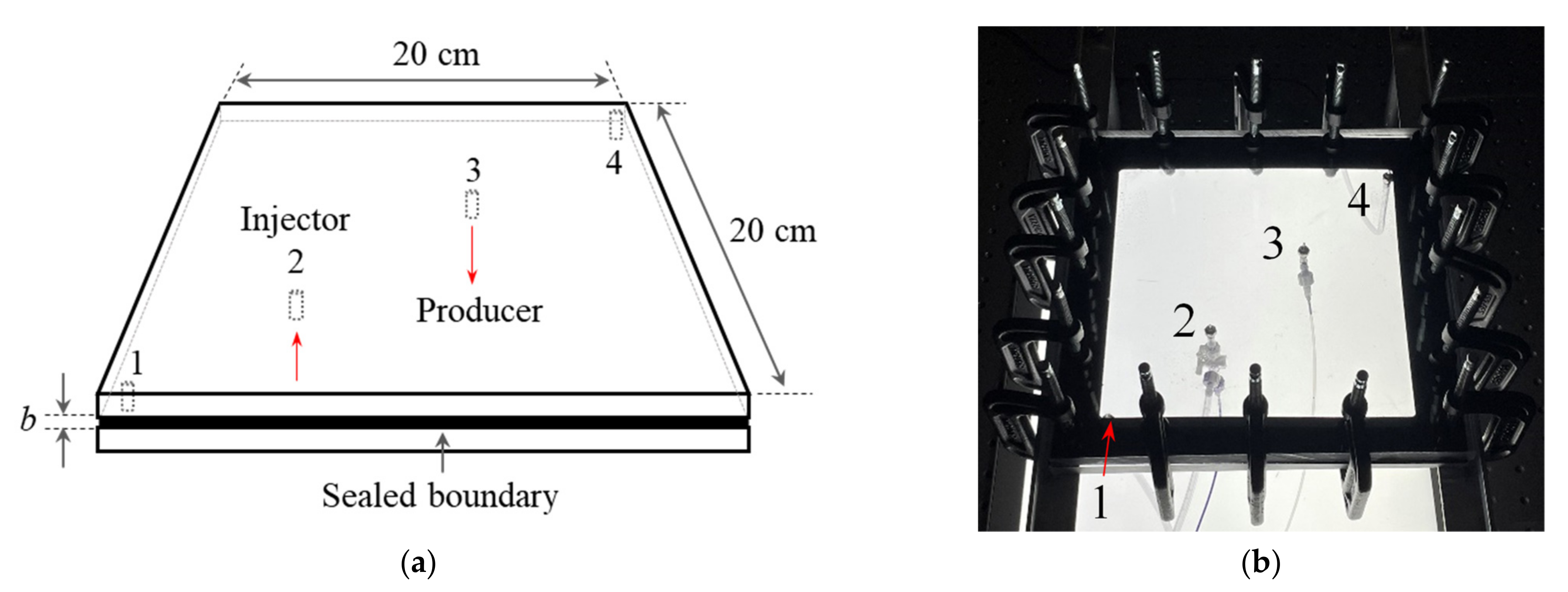
In this section, we will first analyze the flow regimes in miscible displacements at a constant injection rate under the control of constant pressure at outlet. Three new flow regimes are identified and discussed. We then examine how the injection rate affects the VF instabilities and flow regimes. Following that, the impacts of different controls at the production end, i.e., constant pressure vs. constant production rate at outlet, on VF dynamics will be discussed. Both qualitative and quantitative analysis will be performed to better understand the flow dynamics. In most of the following plots for water plumes, only a square of view area incorporating wells 1 to 3 is shown.

3.1. New Flow Regimes

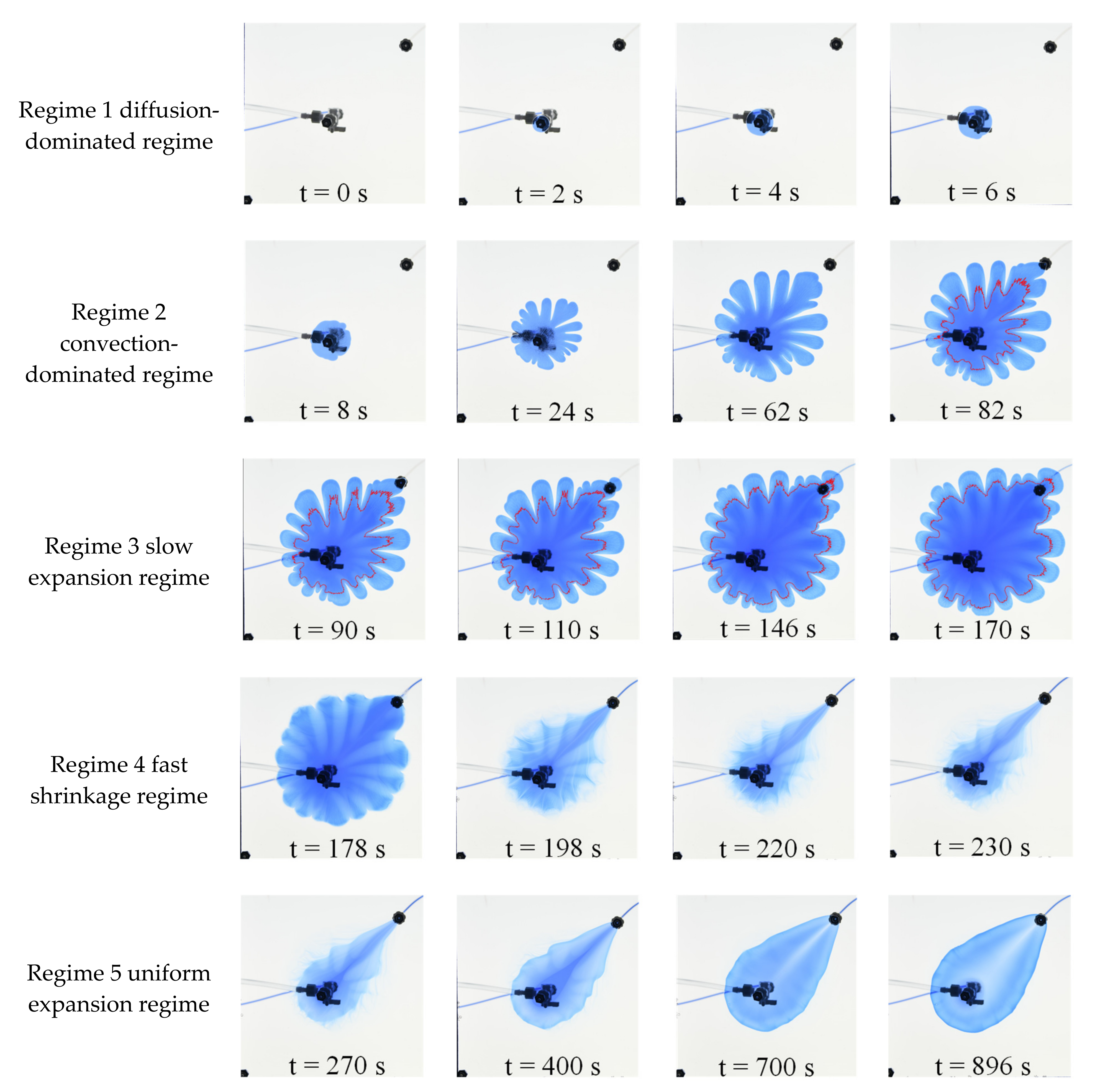
Previous studies on miscible viscous fingering show that flows are first dominated by diffusion at an initial time and then by convection at a later time. Such fingering dynamics result from the competition of these two mechanisms [20,21,36]. The two corresponding regimes are also shown in Figure 2 at a constant injection rate of 5.0 mL/min. Regime 1 (diffusion-dominated regime) starts from initial time to t = 6 s prior to the development of viscous fingering. Regime 2 (convection-dominated regime) is from t = 6 s to breakthrough at t = 82 s, with fingering becoming more unstable with time. During these two regimes, only pure glycerol is produced.

Interestingly, as water injection continues, three new flow regimes are observed following the first two regimes, as shown in Figure 2. Regime 3 starts from breakthrough time t = 82 s when water just reaches to the production well and ends at t = 170 s when the water begins to be produced from the outlet of the tubing. At the end of Regime 3, the water plume reaches the maximum size. This regime seems to be not significantly different from Regime 2 as the water plume continues to expand. However, a careful observation shows that it exhibits different characteristics in terms of fingering structures and dynamics. Specifically, from t = 90 s to t = 170 s, the fingers become shorter with time. The distance between the finger front and the inner water plume (deep blue and highlighted by red outlines) also becomes shorter. This is opposite to the observation in Regime 2. In Regime 3, VF instability is actually suppressed as water is continuously injected. Fingering coalescence happens in the injector-to-producer direction, resulting in a decrease in the count of fingers. In the perpendicular direction, much less fingering coalescence happens, while a minor tip-splitting is observed. Such a slow expansion of water plume is because a proportion of water instantaneously flows out of the Hele–Shaw cell through the production well as water is being injected. Thus, the driving force for water propagation at the water–glycerol interface become weaker compared with that in Regime 2. Overall, the water–glycerol interface grows slowly with stabilized fingers in this new regime. We therefore refer to it as a slow expansion regime.

At t = 170 s, the maximum water plume is achieved. After that, a rapid shrinkage of injected water plume is observed until t = 230 s, which is referred to a fast shrinkage regime. Note that under the control of constant pressure at the outlet, the injection rate is constant, while the pressure at the injector and in the Hele–Shaw continues to increase before water is produced from the outlet. At t = 170 s, the pressure gradient from the injector to outlet is the highest, and the viscosity of fluids along the injector-to-outlet direction is the lowest. According to the Darcy’s law, the production rate will be very fast, resulting in a fast shrinkage of water plume. A clear fluid flow path and backward fingers can be seen at times from t = 198 s to t = 230 s in Figure 2. In this regime, an irregular pattern of water–glycerol interface is achieved with observed residual water distributed outside of the main water plume.

The fast shrinkage of water plume also creates a connection from injector to producer with minimum resistance for injected water to flow. Consequently, most of the injected water will be directly produced. After a relatively long time after t = 230 s, the irregular pattern of the water plume disappears because of the diffusion of two fluids, while a plume with a stable water–glycerol interface appears. With time, this stable plume expands slowly without any viscous fingering (see Figure 2 Regime 5, t = 700 s and t = 896 s). Since most of the injected water is preferentially produced through a production well, it will not contribute to the expansion of the water plume. Instead, the expansion of the water plume results from the mixing of two fluids dominated by molecular diffusion. We, therefore, refer to this stage as a uniform expansion regime. An interesting phenomenon in this regime is that there seems to have a higher concentration of glycerol in the injector-to-producer direction.

The VF dynamics and new flow regimes are also examined quantitively in terms of the variations of swept area and interfacial length between two fluids, as depicted in Figure 3. The software ImageJ is used to determine the interface and their values at different times in each experiment. For immiscible displacements with a clear interface between two fluids, the swept area is expected to increase linearly, as it is proportional to the injection rate and time, regardless of VF instabilities. However, for the miscible case, diffusion plays a role in smoothening the interface of two fluids. For this reason, there is actually no so-called ‘interface’ in miscible displacements. However, for convenience, we use the ‘interface’ or ‘front’ to refer to the evolution of water plume. The variations of swept area also depend on the concentration threshold when determining the interface. As shown in Figure 3, the swept area of water (red dashed curve) increases linearly from initial time to breakthrough. After that, there is a very slight decrease in the slope from t = 82 s to t = 170 s due to the diffusion. Starting from t = 170 s in Regime 4, a sudden drop in water plume area is observed because of the fast shrinkage of the plume. At the end of Regime 4 at time t = 230 s, a minimum water plume area is achieved, which is followed by the slowly increasing stage of uniform expansion dominated by diffusion.

Interestingly, the variations of interfacial length of water plume exhibit different characteristics compared to the swept area. The interfacial length increases quickly in the first two regimes because of the continuous injection of water and viscous finger instabilities. In the subsequent Regime 3, starting at t = 82 s, it slightly decreases. This is because of the stabilized viscous fingers, as indicated in Figure 2 from t = 82 s to 170 s (the start and end times of Regime 3, respectively). This is also an important reason why Regime 3 is separated from other regimes. In the fast shrinkage Regime 4, the interfacial length also decreases dramatically. Interestingly, as water flows to the production well quickly, a fluctuation of interfacial length is clearly observed because of the backward fingers in irregular fingering structures, as shown from t = 170 s to 200 s in Figure 2 and Figure 3. Such backward fingers take effects in a short time because water quickly flows to the production well and mitigates the irregular structures to some extent. Overall, in Regime 4, the interfacial length decreases with time, and the swept area reaches a minimum value at the end of this regime. The backward fingers do not completely disappear even at the beginning of Regime 5. Instead, the more distorted interfaces lead to an increase in interfacial length (see Figure 3e at t = 300 s), although the swept area only slightly increases. Eventually, the interfacial length decreases and then increases extremely slowly as more water is injected and as the water plume expands with time.

The present VF dynamics clearly distinguishes itself from that in five-spot geometry [37], radial geometry [38], and rectangular geometry [36]. With the current well location and Hele–Shaw cell geometry, a non-symmetrical fingering pattern is observed, while the five-spot geometry assumes a symmetrical flow pattern. Interestingly, the present work also shows that small fingers can happen at the opposite side of the injector-to-producer direction due to the pressure gradient. The current case is, therefore, more realistic when only two wells exist in the miscible-based processes in subsurface energy and environment systems. Importantly, the new regimes provide more insights into the performance of the ‘life cycle’ miscible displacements.

We further analyze the fractal dimension of viscous fingering for different regimes based on the evolution of interface in Figure 2 at a water injection rate of 5.0 mL/min. The fractal dimension is obtained by box-counting characterization of the interface depicted by the invading fingers [39]. The Frac box count plugging in ImageJ is used to determine the fractal dimension for each image. Overall, the value of fractal dimension decreases as flows become more unstable with distorted fingers growing with time, while it increases when flows are stabilized [40]. Regime 1 (diffusion dominated regime) is neglected because it is too short at 5.0 mL/min. As shown in Figure 4, the fractal dimension of Regime 2 decreases rapidly as VF becomes more unstable with time. The convective effects are more significant in driving the mixing of two fluids relative to diffusive effects. In contrast, the fractal dimension for Regime 3 generally increases with time, which is consistent with the observation in Figure 2, where fingers become shorter and wider. This also distinguishes it from Regime 2 and confirms the existence of Regime 3. Following that, a rapid decrease in fractal dimension in Regime 4 is observed, resulting from the quick shrinkage and the backward fingers. The mixing in this regime is caused by the fast co-flowing of fluid mixtures to the outlet. As backward fingers are mitigated by diffusion in Regime 5, the variations of fractal dimension become smooth. Diffusion dominates the mixing of two fluids and the expansion of the water plume.

3.2. Impacts of Water Injection Rate

Displacements with several constant water injection rates are performed. Figure 5 shows the water plume at the start and end of different flow regimes at a water injection rate of 1.0 mL/min with constant pressure control at the outlet. Five flow regimes can still be seen in the whole displacement processes, which is similar to those at 5.0 mL/min in Figure 2. However, different characteristics are also observed when the injection rate decreases to 1.0 mL/min. Generally, at a lower injection rate, the VF is less unstable with apparently shorter fingers at a breakthrough time of t = 358 s and at the start of the shrinkage stage t = 476 s. The count of fingers is also less at a lower injection rate. Compared to Figure 2 where fingers are noticeably stabilized in a slow expansion stage (t = 82 s to 170 s), the stabilizing effect at 1.0 mL/min is however much weaker. At the end of the shrinkage stage at t = 566 s, the size of the water plume at 1.0 mL/min is larger than that of 5.0 mL/min and is less irregular. In fact, when the injection rate is as low as 0.1 mL/min, neither the stabilizing effect nor the shrinkage of water plume is obvious.

The impacts of injection rates are also examined by comparing the VF dynamics when 2.5 mL of water is injected, as depicted in Figure 6. The Péclet number Pe is defined as $\mathrm{Pe}=\mathrm{q}/\left(2\mathsf{\pi }\mathrm{bD}\right)$, where q is the volumetric flow rate of injection varying from 0.1 mL/min to 5.0 mL/min. D is the diffusivity between water and glycerol, which is 1.6 × 10⁻¹⁰ m²/s [13,41]. Overall, at a lower injection rate with a smaller Pe, the water plume is less unstable, and VF mainly develops in the injector-to-producer direction due to the higher pressure gradient in this direction. While on the opposite side of the injector-to-producer direction, the water–glycerol interface propagates stably at a lower injection rate. On the contrary, at a higher injection rate with a larger Pe, small fingers can still develop on the opposite side of the injector-to-producer direction. Another observation is that a larger swept area is achieved at a lower injection rate because of the longer period of time for injecting 2.5 mL water and the smaller water plume. For example, 1800 s is needed to inject 2.5 mL water at an injection rate of 0.1 mL/min. For such a long time, diffusion plays a role in enabling more expansion of the water plume, thus resulting in a larger swept area and less concentration gradient in the water plume.

We further examine water injection rates on the shape of the water plume, as depicted in Figure 7. When breakthrough happens in Figure 7a, the flows are apparently more unstable at a higher injection rate because of stronger convection. On the contrary, at a higher injection rate, the minimum size of the water plume at the end of the shrinkage stage is smaller, as shown in Figure 7b. This is because during the shrinkage stage the stronger convection mobilizes the water plume to the production well quickly under a larger pressure gradient from injector to producer. For the highest injection rate at 5.0 mL/min, the shrinkage rate is so fast that the irregular shape of the water plume is clearly observed with a flow path from the water–glycerol interface to producer, not only along the injection–producer. Water and glycerol are further mixed because of this quick shrinkage. When the injection rate is less than or equal to 0.5 mL/min, the minimum size of the water plume becomes insensitive to the water injection rate. Interestingly, for slower injection rates, some residual glycerol seems to be formed in the injector-to-producer direction indicated by the slight white color. Different from its counterpart at high injection rates, the change of glycerol concentration along the injector–producer direction is not obvious from breakthrough to the end of slow expansion at a low water injection rate. In addition, we have observed the backward fingers in the producer-to-injector direction in Figure 2, Figure 6 and Figure 7. They are caused by the larger pressure gradient at only higher water injection rates.

From the color of water plumes in Figure 7a, it can be seen that the viscosity of the water plume at a higher injection rate is apparently lower than that at a lower rate when breakthrough happens. This also leads to a large pressure gradient between the injector and producer according to Darcy’s law, which is another reason for the fast shrinkage of the water plume at a higher injection rate.

The influences of water injection rates on VF dynamics can also be quantified by the variations of swept areas, as depicted in Figure 8. It is clear that the slope of the swept area with time increases with the injection rate of water. Interestingly, the slope of the swept area with the volume of water injected however decreases with the injection rates before the maximum water plume is achieved in Figure 8b. This is because of the relatively weaker diffusion compared to the increasingly stronger convection at a higher rate. However, at the end of the slow expansion regime, the maximum size of the water plume increases with the injection rate. A non-monotonic relationship between the size of the water plume and injection rates is observed at the end of the shrinkage regime. At a very small injection rate, the shrinkage period is short, and the decrease in water plume is not obvious. Therefore, a larger maximum water plume size in the previous slow expansion stage leads to a larger minimum shrinkage size. However, at the higher injection rate, e.g., 2.0 mL/min and 5.0 mL/min, the stronger convection is favorable for the shrinkage of water plume, resulting in a smaller water plume at the end of the shrinkage regime.

Different water injection rates lead to unstable flows, which can be quantified by the evolution of count of fingers as water is injected to displace glycerol. As shown in Figure 9, under constant pressure control at the outlet, a higher flow rate induces more fingers because of the stronger convection. The maximum count of fingers is reached at an earlier time for a higher water injection rate. Interestingly, less fluid is needed to reach the maximum count of fingers, as shown in Figure 9b. Eventually, the count of fingers tends to be zero because of the formation of a stable and smooth interface in the uniform expansion regime.

3.3. Impacts of Control at the Outlet

Experiments with constant production rate control are performed. Figure 10 depicts the water plume at the beginning and end of the five flow regimes for water injection rates of 5.0 mL/min and 2.0 mL/min, respectively. The main effects occur at the breakthrough and following regimes occur after breakthrough. Because of the constant production rate control at the outlet, the injected water propagates much faster than that under a constant pressure control scenario at the outlet. This is confirmed by a significant reduction in breakthrough time at each injection rate. Furthermore, at 5.0 mL/min, the size of Regime 3 is smaller than that of constant pressure control. The interface of the water plume of Regime 4 is less unstable with fewer backward fingers (see Figure 10a at t = 132 s vs. Figure 2 at t = 130 s). For 2.0 mL/min, the duration of a slow expansion regime and fast shrinkage regime is greatly reduced, and the shrinkage regime is not obvious at all. In fact, for water injection rates at 1.0 mL/min, 0.5 mL/min, 0.2 mL/min and 0.1 mL/min, the shrinkage regime and expansion regime are negligible. So, the differences between the two control scenarios at the outlet are not obvious at slow water injection rates.

Figure 11 depicts the variations of swept area with time for the two scenarios with different controls at the outlet. The control with a constant production rate (two-pump scenario) initially shows the same trend of swept area of injected water. As seen in Figure 11a, the solid and dotted curves nearly overlap for a short time. However, the breakthrough and the time for the maximum size of the water plume occur at an earlier time, when the size of the water plume is much smaller for the two-pump scenario. This indicates that the constant extraction by the additional pump at the outlet may induce an extra pressure gradient from the injector to producer that is favorable for the injected water flowing to the production end. This also suppresses the expansion of the water plume in other directions. At the injection rate of 5.0 mL/min, this results in a much smaller water plume (i.e., 6641 mm² vs. 13,060 mm²). At the injection rate of 2.0 mL/min, the water plume for the two-pump scenario is also much smaller. Both scenarios lead to a comparable size of water plume at the end of the fast shrinkage regime for an injection rate of 5.0 mL/min. At a small injection rate of 2.0 mL/min, the shrinkage regime for the two-pump scenario is however not noticeable. A much larger, stable water plume is observed as water is continuously injected during the following slow expansion regime for the two-pump scenario, as shown in Figure 10a at t = 132 s and Figure 10b at t = 220 s.

Although the swept area for different controls at the outlet is significantly different, the interfacial length is however close for the two scenarios at the same injection rate, as shown in Figure 11b. This is because the scenario with a constant production rate at the outlet (two pumps) does not reduce the VF instabilities too much. Instead, it mainly affects the spreading direction of injected water, with a preferential flow path from the injector to producer. This also results in an early breakthrough time. Another interesting observation in Figure 11b is that the backward fingering is mitigated to some extent because of the constant production control, which is indicated by the lower fluctuations on the variations of interfacial length vs. time (i.e., the dotted curves in Figure 11b). At an injection rate of 2.0 mL/min, the backward fingering as well as the fluctuations of interfacial length are much weaker.

Two interesting phenomena were observed through the analysis of the variations of count of fingers with time in Figure 12. First, at a lower flow rate, a large number of small, uniform fingers are observed (see Figure 12 at t = 282 s for 0.1 mL/min). Along the injector-to-producer direction (i.e., the main flow direction), these fingers are induced by convection. In contrast, along the producer-to-injector direction and in the transverse direction, the water flow rate is very slow. Spontaneous fingers are formed due to the diffusion and possibly the small but non-zero interfacial tension between two fluids [42]. Second, the maximum count of fingers is achieved at a water injection rate of 1.0 mL/min for the control of a constant production rate at the outlet, which is different from its counterpart at constant pressure control at the outlet in Figure 9a. Below this rate, the small, spontaneous fingers tend to merge with each other as water is injected continuously (see 0.1 mL/min vs. 0.2 mL/min in Figure 13a,b, respectively). In the case of higher flow rates, tip splitting is more obvious. However, the coalesces among these fingers lead to long and wide fingers (see Figure 13 for 2.0 mL/min and 5.0 mL/min). Therefore, the highest injection rate does not lead to the maximum count of fingers. Eventually, the maximum count of fingers happens at the water injection rate of 1.0 mL/min.

To sum up, the design of experiments, flow regimes, and different controls at the production end in the present work provide new insights to the applications such as oil and gas recovery, geothermal recovery, and CO₂ and hydrogen geological storage. More specifically, the design of an injector–producer Hele–Shaw cell and sealed boundary allows examining the post-breakthrough fingering dynamics and flow regimes, which cannot be achieved using the classical radial geometry. The tubing connected to the producer mimics the effect of wellbore on flow dynamics in reservoirs. The different controls on the production end lead to different flow dynamics, which should be considered in the design of field projects. Last but not least, the new design of experiments, i.e., two wells inside the geometry, distinguishes from classical five-spot geometry and expands the capability of the Hele–Shaw cell for studying the non-symmetric flows in a variety of applications.

4. Conclusions

In this paper, we present the experimental results for the full ‘life cycle’ of miscible viscous fingering in a sealed Hele–Shaw cell, with particular interests in spatial and temporal variations of fingering dynamics. The effect of geometry, water injection rates, and pressure and rate controls at the outlet is investigated.

Based on qualitative and quantitative analysis, we identified five flow regimes: (1) a diffusion-dominated regime, (2) a convection-dominated regime with significant fingering instability, (3) a slow expansion regime before breakthrough, (4) a fast shrinkage regime immediately after breakthrough, and (5) a uniform expansion regime without fingering instability. The last three regimes are reported for the first time and confirmed by the characterization of fractal dimension. Such new characteristics of miscible displacements distinguish the current work from previous studies and provide new insights into flow dynamics in a Hele–Shaw cell and in porous media.

The water injection rate plays a role in affecting the fingering dynamics, flow regimes, swept area, interfacial length, and count of fingers in the whole displacements. The variations of expansion and shrinkage regimes are more significant at a higher water injection rate. Interestingly, the smallest water plume with the most irregular backward fingers is achieved by the fastest injection rate at the end of the shrinkage regime.

The two injection scenarios, i.e., constant pressure vs. constant production rate control at outlet, have more pronounced impacts on flow dynamics especially at large injection rates. For the scenario with a constant production rate at the outlet, the expansion and shrinkage regimes are less significant compared to its counterpart at constant pressure control. In addition, for the scenario with a constant production rate, the maximum count of fingers is obtained at the water injection rate of 1.0 mL/min. Below it, spontaneous fingers are formed, while above this injection rate, small fingers tend to merge with larger fingers.

The current work identifies new flow regimes, quantifies their characteristics, and reports interesting VF dynamics in miscible displacements. It provides new insights into the fundamental mechanisms of miscible developments in a variety of applications such as CO₂ sequestration, hydrogen storage, enhanced oil recovery, and groundwater contaminate remediation.

References

1. Huppert, H.E.; Neufeld, J.A. The fluid mechanics of carbon dioxide sequestration. Annu. Rev. Fluid Mech. 2014, 46, 255–272. [Google Scholar] [CrossRef]
2. Heinemann, N.; Scafidi, J.; Pickup, G.; Thaysen, E.M.; Hassanpouryouzb, A.; Wilkinson, M.; Satterley, A.K.; Booth, M.G.; Edlmann, K.; Haszeldine, R.S. Hydrogen storage in saline aquifers: The role of cushion gas for injection and production. Int. J. Hydrogen Energy 2021, 46, 39284–39296. [Google Scholar] [CrossRef]
3. Lake, L.W. Enhanced Oil Recovery; Prentice: Hoboken, NJ, USA, 1989; pp. 86–123. [Google Scholar]
4. Welty, C.; Allen, C.; Kane III, A.C.; Kauffman, L.J. Stochastic analysis of transverse dispersion in density-coupled transport in aquifers. Water Resour. Res. 2003, 39, 1150. [Google Scholar] [CrossRef]
5. Rana, S.; Ardichvili, A.; Tkachenko, O. A theoretical model of the antecedents and outcomes of employee engagement: Dubin’s method. J. Workplace Learn. 2014, 26, 249–266. [Google Scholar] [CrossRef]
6. Hill, S. Channeling in packed columns. Chem. Eng. Sci. 1952, 1, 247–253. [Google Scholar] [CrossRef]
7. Saffman, P.G.; Taylor, G.I. The penetration of a fluid into a porous medium or Hele-Shaw cell containing a more viscous liquid. Proc R Soc Lond A Math Phys. Sci. 1958, 245, 312–329. [Google Scholar] [CrossRef]
8. Homsy, G.M. Viscous fingering in porous media. Ann. Rev. Fluid Mech. 1987, 19, 271–311. [Google Scholar] [CrossRef]
9. Chen, J.D. Radial viscous fingering patterns in Hele-Shaw cells. Exp. Fluids 1987, 5, 363–371. [Google Scholar] [CrossRef]
10. McCloud, K.V.; Maher, J.V. Experimental perturbations to Saffman-Taylor flow. Phys. Rep. 1995, 260, 139–185. [Google Scholar] [CrossRef]
11. Kargozarfard, Z.; Riazi, M.; Ayatollahi, S. Viscous fingering and its effect on areal sweep efficiency during waterflooding: An experimental study. Pet. Sci. 2019, 16, 105–116. [Google Scholar] [CrossRef]
12. Kozlov, V.; Karpunin, I.; Kozlov, N. Finger instability of oscillating liquid–liquid interface in radial Hele-Shaw cell. Phys Fluids 2020, 32, 102. [Google Scholar] [CrossRef]
13. Suzuki, R.X.; Quah, F.W.; Ban, T.; Mishra, M.; Nagatsu, Y. Experimental study of miscible viscous fingering with different effective interfacial tension. AIP Advances 2020, 10, 115–219. [Google Scholar] [CrossRef]
14. Petitjeans, P.; Chen, C.Y.; Meiburg, E.; Maxworthy, T. Miscible quarter five-spot displacements in a Hele-Shaw cell and the role of flow-induced dispersion. Phys. Fluids 1999, 11, 1705–1716. [Google Scholar] [CrossRef]
15. Fernandez, J.; Kurowski, P.; Petitjeans, P.; Meiburg, E. Density-driven unstable flows of miscible fluids in a Hele-Shaw cell. J. Fluid Mech. 2002, 451, 239–260. [Google Scholar] [CrossRef]
16. Jiao, C.; Maxworthy, T. An experimental study of miscible displacement with gravity-override and viscosity-contrast in a Hele Shaw cell. Exp. Fluids 2008, 44, 781–794. [Google Scholar] [CrossRef]
17. Singh, A.; Singh, Y.; Pandey, K.M. Viscous fingering instabilities in radial Hele-Shaw cell: A review. Mater. Today Proc. 2020, 26, 760–762. [Google Scholar] [CrossRef]
18. Rana, C.; Mishra, M. Fingering dynamics on the adsorbed solute with influence of less viscous and strong sample solvent. J. Chem. Phys. 2014, 141, 214701. [Google Scholar] [CrossRef]
19. Keable, D.; Jones, A.; Krevor, S.; Muggeridge, A.; Jackson, S.J. The effect of viscosity ratio and Peclet number on miscible viscous fingering in a Hele-Shaw cell: A combined numerical and experimental study. Transp. Porous Media 2022, 143, 23–45. [Google Scholar] [CrossRef]
20. Lei, T.; Luo, K.H. Pore-scale study of dissolution-driven density instability with reaction A + B C in porous media. Phys. Rev. Fluids 2019, 4, 063907. [Google Scholar] [CrossRef]
21. Rana, C.; De Wit, A. Reaction-driven oscillating viscous fingering. Chaos 2019, 29, 043115. [Google Scholar] [CrossRef]
22. Lei, T.; Luo, K.H. Pore-scale simulation of miscible viscous fingering with dissolution reaction in porous media. Phys. Fluids 2021, 33, 034134. [Google Scholar] [CrossRef]
23. Videbæk, T.E.; Nagel, S.R. Diffusion-driven transition between two regimes of viscous fingering. Phys. Rev. Fluids 2019, 4, 033902. [Google Scholar] [CrossRef]
24. Nijjer, J.S.; Hewitt, D.R.; Neufeld, J.A. The dynamics of miscible viscous fingering from onset to shutdown. J. Fluid Mech. 2018, 837, 520–545. [Google Scholar] [CrossRef]
25. Etrati, A.; Frigaard, I.A. Viscosity effects in density-stable miscible displacement flows: Experiments and simulations. Phys Fluids 2018, 30, 123104. [Google Scholar] [CrossRef]
26. Coutinho, Í.M.; Miranda, J.A. Control of viscous fingering through variable injection rates and time-dependent viscosity fluids: Beyond the linear regime. Phys. Rev. E 2020, 102, 063102. [Google Scholar] [CrossRef]
27. Sajjadi, M.; Azaiez, J. Scaling and unified characterization of flow instabilities in layered heterogeneous porous media. Phys. Rev. E 2013, 88, 033017. [Google Scholar] [CrossRef]
28. Ruith, M.; Meiburg, E. Miscible rectilinear displacements with gravity override. Part 1. Homogeneous porous medium. J. Fluid Mech. 2000, 420, 225–257. [Google Scholar] [CrossRef]
29. Fahandezhsaadi, M.; Amooie, M.A.; Hemmati-Sarapardeh, A.; Ayatollahi, S.; Schaffie, M.; Ranjbar, M. Laboratory evaluation of nitrogen injection for enhanced oil recovery: Effects of pressure and induced fractures. Fuel 2019, 253, 607–614. [Google Scholar] [CrossRef]
30. Wu, Y.; Li, P. The potential of coupled carbon storage and geothermal extraction in a CO2-enhanced geothermal system: A review. Geotherm. Energy 2020, 8, 19. [Google Scholar] [CrossRef]
31. Tsuzuki, R.; Ban, T.; Fujimura, M.; Nagatsu, Y. Dual role of surfactant-producing reaction in immiscible viscous fingering evolution. Phys. Fluids 2019, 31, 022102. [Google Scholar] [CrossRef]
32. Bunton, P.; Marin, D.; Stewart, S.; Meiburg, E.; De Wit, A. Schlieren imaging of viscous fingering in a horizontal Hele-Shaw cell. Exp. Fluids. 2016, 57, 28. [Google Scholar] [CrossRef]
33. Chevalier, C.; Ben Amar, M.; Bonn, D.; Lindner, A. Inertial effects on Saffman-Taylor viscous fingering. J. Fluid Mech. 2006, 552, 83–97. [Google Scholar] [CrossRef]
34. Caudle, B.H.; Witte, M.D. Production potential changes during sweep-out in a five-spot system. J. Pet. Technol. 1959, 12, 63–65. [Google Scholar] [CrossRef]
35. Schneider, C.A.; Rasband, W.S.; Eliceiri, K.W. NIH Image to ImageJ: 25 years of image analysis. Nat. Methods 2012, 9, 671–675. [Google Scholar] [CrossRef] [PubMed]
36. Tan, C.T.; Homsy, G.M. Simulation of nonlinear viscous fingering in miscible displacement. Phys. Fluids 1988, 31, 1330–1338. [Google Scholar] [CrossRef]
37. Djabbarov, S.; Alistair, D.J.; Samuel, K.; Muggeridge, A.H. Experimental and numerical studies of first contact miscible injection in a quarter five spot pattern. In Proceedings of the SPE Europec featured at 78th EAGE Conference and Exhibition, Vienna, Austria, 30 May 2016. [Google Scholar] [CrossRef]
38. Pihler-Puzović, D.; Peng, G.; Lister, J.; Heil, M.; Juel, A. Viscous fingering in a radial elastic-walled Hele-Shaw cell. J. Fluid Mech. 2018, 849, 163–191. [Google Scholar] [CrossRef]
39. Foroutan-Pour, K.; Dutilleul, P.; Smith, D.L. Advances in the implementation of the box-counting method of fractal dimension estimation. Appl. Math. Comput. 1999, 105, 195–210. [Google Scholar] [CrossRef]
40. Aryana, S.A.; Kovscek, A.R. Experiments and analysis of drainage displacement processes relevant to carbon dioxide injection. Phys. Rev. E 2012, 86, 066310. [Google Scholar] [CrossRef]
41. Petitjeans, P.; Maxworthy, T. Miscible displacements in capillary tubes. Part 1. Experiments. J. Fluid Mech. J. Fluid Mech. 1996, 326, 37–56. [Google Scholar] [CrossRef]
42. Song, W.; Ramesh, N.N.; Kovscek, A.R. Spontaneous fingering between miscible fluids. Colloids Surfaces A Physicochem. Eng. Asp. 2020, 584, 123943. [Google Scholar] [CrossRef]
Figure 1. Experimental setup. Note four wells are located on the lower plate. (a) Schematic of view area of a Hele–Shaw cell. (b) Actual Hele–Shaw cell setup.
Energies 15 05798 g001
Figure 2. Different flow regimes at 5.0 mL/min at constant pressure control at the outlet.
Energies 15 05798 g002
Figure 3. The swept area and interfacial length of water plume for 5.0 mL/min. Fingering outlines are plotted for each regime.
Energies 15 05798 g003
Figure 4. Variations of fractal dimension of viscous fingering.
Energies 15 05798 g004
Figure 5. Flow regime at 1.0 mL/min with constant pressure control at the outlet.
Energies 15 05798 g005
Figure 6. Water plume at 2.5 mL injected water for different injection rates under constant pressure control at the outlet.
Energies 15 05798 g006
Figure 7. Viscous fingering for different injection rates under constant pressure control at the outlet. (a) at breakthrough time; (b) at the end of fast shrinkage regime.
Energies 15 05798 g007aEnergies 15 05798 g007b
Figure 8. Variations of swept area for different injection rates and volume of water injected. (a) Swept area vs. time; (b) Swept area vs. volume of water injected; (c) The viscous fingering at the maximum swept area for different injection rates.
Energies 15 05798 g008
Figure 9. Count of fingers vs. time at different flow rates under constant pressure control at the outlet. (a) Count of fingers vs. time; (b) Count of fingers vs. volume of water injected.
Energies 15 05798 g009
Figure 10. Water plumes at the end of reach regime with constant production rate control at the outlet. (a) Five regimes at 5.0 mL/min; (b) Five regimes at 2.0 mL/min.
Energies 15 05798 g010aEnergies 15 05798 g010b
Figure 11. Comparison of constant pressure control at the outlet (one pump) and constant production rate at the outlet (two pumps) scenarios at two different water injection rates. (a) Swept area vs. time; (b) Interfacial length vs. time.
Energies 15 05798 g011
Figure 12. Count of fingers with time at different flow rates with the control of constant production rate at the outlet (two-pump scenario).
Energies 15 05798 g012
Figure 13. Water plumes at fixed volume of water injected for the control of constant production rate at outlet: (a) at 1.5 mL water injected; (b) at 2.5 mL water injected.
Energies 15 05798 g013
Publisher’s Note: MDPI stays neutral with regard to jurisdictional claims in published maps and institutional affiliations.