SOC Estimation of Lithium-Ion Battery Based on Equivalent Circuit Model with Variable Parameters

Abstract

The state of charge (SOC) of the battery is an important basis for the battery management system to perform state monitoring and control decisions. In this paper, by identifying the internal parameters of the battery model at different temperatures and SOCs of the lithium-ion battery, the specific factors that affect the change of the parameters are analyzed, the segmentation basis of the model and the fitting method of related parameters are discussed, the second-order equivalent circuit model of the lithium-ion battery whose parameters vary with SOC and temperature is established, the unscented Kalman filter (UKF) is used to estimate the SOC of the lithium-ion battery, and an improved SOC estimation method based on optimized equivalent circuit model is proposed. Simulation and experimental results show that the improved SOC estimation strategy can obtain high estimation accuracy in a wide temperature range.

1. Introduction

The power lithium-ion battery has become a research hotspot in the electric vehicle industry because of its high energy density, low self-discharge, good safety performance, and long life [1,2]. In [3], a new material for lithium batteries was proposed to improve the energy of lithium batteries. In article [4], a new lithium battery structure was designed, which can effectively avoid the influence of temperature on battery parameters and improve battery energy utilization rates. On this basis, battery management technology also needs to be studied. A battery management system (BMS) can monitor and manage the working state of a power battery, making the battery run safely and reliably, improving the life of the battery, and extending the cruising range of the electric vehicle. The state of charge (SOC), which is a physical quantity representing the amount of energy left in a battery, is an important basis for BMS to monitor the status of the battery and control decision making [5]. Therefore, SOC estimation has become a key part of the effective operation of BMSs.

At present, the SOC estimation for power batteries mainly focuses on two aspects. Firstly, the equivalent model of batteries is studied. At present, the main battery models include the electrochemical model [6], the equivalent circuit model [7], the black box model [8], and the battery thermal model [9]. The electrochemical model has higher accuracy, but there are many model parameters, and most of the parameters are affected by the material, structure, and size of the battery. The black box model is simple and flexible, which is suitable for practical use. However, considering its high requirements for the quantity and quality of sample data, it needs more mature development. Although the battery thermal model has some research on battery heat generation, it cannot accurately reflect the heat generation and temperature rise pattern of the internal structure of large power lithium-ion batteries. The equivalent circuit model can well describe the electrochemical reaction with the circuit, which is suitable for a variety of batteries. However, its accuracy largely depends on the design of the specific equivalent circuit and the accuracy of parameter identification.

Secondly, the research aims at SOC itself. The SOC estimation methods mainly include the ampere-time integral method [10], neural networks [11], the particle filter (PF) algorithm [12,13,14], and the Kalman filter (KF) and its improved algorithm [15,16,17,18,19,20]. The ampere-time integral method is easy to implement, but it does not have feedback correction, so there will be accumulated errors. The neural network method is suitable for the simulation of highly nonlinear systems, but establishing an accurate network needs a lot of data to train and the training process is usually time-consuming. The filtering method (i.e., PF and KF mentioned above) can continuously modify the estimated value in the iterative process, which has a good suppression effect on the system noise, but it relies largely upon the accuracy of the underlying battery models.

Temperature changes have a great impact on the performance of lithium-ion batteries. The capacity, terminal voltage, and internal resistance of the battery are all affected by temperature, which brings a lot of inconvenience to the use of power batteries. Poor estimations have been reported for SOC at low temperatures [21]. Therefore, the influence of temperature must be considered when estimating the SOC of batteries.

In this paper, the battery capacity test and the hybrid pulse power characteristic (HPPC) test are carried out at different temperatures to obtain the characteristics of the battery. This paper analyzes the influence of different SOCs and temperatures on the open-circuit voltage, ohmic internal resistance, polarization resistance, and polarization capacitance of lithium-ion batteries. Based on this, an equivalent circuit model adapting to temperature and SOC changes is established, and the UKF algorithm is used to accurately estimate SOC.

The rest of this paper is organized as follows: In Section 2, the equivalent circuit model of the battery is established, the ohmic resistance and polarization parameters of the battery are identified, and UDDS working conditions are used to verify the model at different temperatures. In Section 3, an SOC estimation algorithm based on UKF is proposed and verified. Finally, Section 4 concludes this article.

2. Establishment of Battery Equivalent Model

2.1. Second-Order RC Equivalent Circuit Model

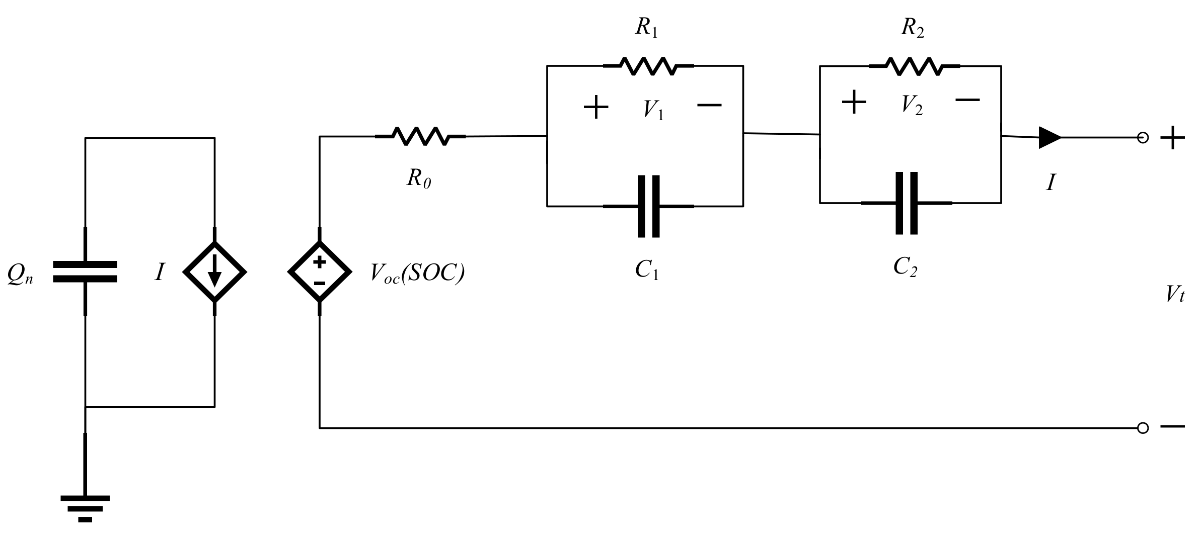
This paper adopts the second-order RC equivalent circuit model [22] to analyze the battery characteristics. As shown in Figure 1, $Q_n$ is the battery’s nominal capacity and indicates the total energy stored in the battery. $V_t$, $I$ represent terminal voltage and current (it is positive when discharging and negative when charging). SOC represents the ratio of the available capacity to the nominal capacity of the battery [23], as shown in Equation (1).

$$SOC\left(t\right)=SOC\left(t_0\right)-\frac{1}{Q_n}{\displaystyle {\int }_{t_0}^{t}I\left(t\right)}dt$$

(1)

$SOC\left(t_0\right)$ is the SOC at time $t_0$. $V_{oc}$ (the voltage across $Q_n$) changes with the SOC variations from 0% to 100%. The controlled voltage source $V_{oc}\left(SOC\right)$ reflects the nonlinear relationship between SOC and open-circuit voltage (OCV). $R_0$ is the ohmic resistance. $R_1\parallel C_1$ represents electrochemical polarization, describing the structure of the electric double layer at the electrode or solution interface. $R_2\parallel C_2$ indicates concentration polarization. The electrical characteristic of the equivalent circuit model can be described as follows:

$$\begin{array}{l}{V}_t=V_{oc}\left[SOC(t)\right]-V_1(t)-V_2\left(t\right)-I\left(t\right)\cdot R_0\\ I\left(t\right)=\frac{V_1\left(t\right)}{R_1}+C_1\frac{d{V}_1\left(t\right)}{dt}\\ I\left(t\right)=\frac{V_2\left(t\right)}{R_2}+C_2\frac{d{V}_2\left(t\right)}{dt}\end{array}$$

(2)

The terminal voltage $V_t$ and current $I$ are taken as the output $y$ and input $u$ of the equivalent circuit model, respectively. SOC, $V_1$ and $V_2$ are state variables. Discretizing Equations (1) and (2), the state-space equation of the second-order RC equivalent circuit model is as follows:

$$\begin{array}{l}x\left(k+1\right)=A\cdot x\left(k\right)+B\cdot u\left(k\right)\\ y\left(k\right)=C\cdot x\left(k\right)+D\cdot u\left(k\right)\end{array}$$

(3)

In the Equation (3), $x\left(k\right)={\left[\begin{array}{ccc}SOC(k)& V_1(k)& V_2\left(k\right)\end{array}\right]}^T$, $u\left(k\right)=I\left(k\right)$, $y\left(k\right)=V_t\left(k\right)$, $A=\left[\begin{array}{ccc}1& 0& 0\\ 0& \exp \left(-\frac{\Delta t}{{\tau }_1\left(k\right)}\right)& 0\\ 0& 0& \exp \left(-\frac{\Delta t}{{\tau }_2\left(k\right)}\right)\end{array}\right]$, $B=\left[\begin{array}{c}-\frac{\Delta t}{Q_n}\\ R_1\left(k\right)\cdot \left(1-\exp \left(-\frac{\Delta t}{{\tau }_1\left(k\right)}\right)\right)\\ R_2\left(k\right)\cdot \left(1-\exp \left(-\frac{\Delta t}{{\tau }_2\left(k\right)}\right)\right)\end{array}\right]$, $C=\left[\begin{array}{ccc}\frac{\partial V_{oc}\left[SOC(k)\right]}{\partial SOC\left(k\right)}& -1& -1\end{array}\right]$, $D=-R_0$, $\Delta t$ is the interval of sampling time, $\tau$ represents the time constant, ${\tau }_1=R_1{C}_1$, ${\tau }_2=R_2{C}_2$.

The second-order RC equivalent circuit model described by the Equation (3) will be used for the SOC estimation of batteries in the following section.

2.2. Parameter Identification and Fitting

The battery used in this paper is a ternary lithium-ion battery with a nominal capacity of 2800 mAh. The experimental equipment used in the test include a Neware charging and discharging machine, programmable temperatures, and a humidity chamber. According to the operating temperature range of the lithium-ion battery, when testing the battery, the experimental environment temperatures −10 °C, 0 °C, 10 °C, 20 °C, 25 °C, 30 °C, 40 °C, and 50 °C were chosen. Five batteries were placed under each temperature.

2.2.1. Open-Circuit Voltage

Since the open-circuit voltage (OCV) of charging is a little higher than that of discharging, the OCV of lithium-ion batteries at different temperatures and SOCs is measured by averaging the two values, as shown in Figure 2.

Figure 2 demonstrates that the OCV is affected by the ambient temperature. When the temperature T > 10 °C, the OCV decreases slowly with the increase of temperature, and the variation range is small. When T ≤ 10 °C, the open-circuit voltage decreases obviously with the increase of temperature, especially when the SOC of the battery is close to 0. Therefore, the influence of temperature and SOC on the OCV of a ternary lithium-ion battery cannot be ignored and should be fully considered when building the battery model.

The Curve Fitting Toolbox in MATLAB was used to establish the functional relationship of OCV related to SOC and temperature T.

$$\begin{array}{l}OCV\left(SOC,T\right)=p00+p10\cdot T+p01\cdot SOC+p20\cdot T^2+\\ \begin{array}{cccc}& & & \end{array}\begin{array}{cc}& \end{array}p11\cdot T\cdot SOC+p02\cdot SO{C}^2+p30\cdot T^3+\\ \begin{array}{cccc}& & & \end{array}\begin{array}{cc}& \end{array}p21\cdot T^2\cdot SOC+p12\cdot T\cdot SO{C}^2+p03\cdot SO{C}^3\end{array}$$

(4)

The values of the fitting coefficients are shown in

Table 1. Values of the coefficients in the OCV-SOC-T function.

$\mathit{p}00$	$\mathit{p}10$	$\mathit{p}01$	$\mathit{p}20$	$\mathit{p}11$
3.396	−0.0050	−0.759	7.5 × 105	−0.0084
$\mathit{p}02$	$\mathit{p}30$	$\mathit{p}21$	$\mathit{p}12$	$\mathit{p}03$
−0.4252	−1.30 × 107	8.96 × 105	−0.0022	−0.4373

.

2.2.2. Ohmic Internal Resistance

The ohmic internal resistance of equivalent circuit under different temperatures and SOCs is identified accurately by a hybrid pulse power characteristic (HPPC) test. Figure 3 shows the voltage change (point a → point b) under a pulse discharge in the HPPC test. In the figure, the voltage is recorded every 0.1 s. The battery is at rest before point a. Between point a and c, the battery is discharged at a constant current of 1C for 10 s. Between point c and e, the battery is rested again.

At the beginning (point a → point b) and end (point c → point d) of its discharge, the terminal voltage of lithium-ion battery will jump up and down. This phenomenon is caused by the ohmic internal resistance [24]. The average of the voltage difference between two segments was taken to reduce the identification error. The calculation formula is shown in Equation (5). The change of ohmic internal resistance at different temperatures and SOC is shown in Figure 4.

$$R_0=\frac{\left|V_T\left(t_b\right)-V_T\left(t_a\right)\right|+\left|V_T\left(t_d\right)-V_T\left(t_c\right)\right|}{2\left|I_T\right|}$$

(5)

Figure 4 shows that both temperature and SOC changes can affect R₀, especially when the ambient temperature is low. When the temperature is fixed, R₀ increases slowly with the decrease of SOC, the numerical fluctuation is more obvious at low temperatures. Under the same SOC, R₀ is increasing with the decrease of temperature, the change rate gradually increases. It is calculated that the value of R₀ at −10 °C is about 3 times higher than that at 25 °C, while at 25 °C, it is only 1.37 times of that at 55 °C.

As shown in Figure 5a, the effect of temperature on R₀ is much greater than that of SOC. The change of R₀ with SOC is not obvious at the same temperature, but the change of temperature will cause a significant fluctuation. The changing rate of R₀ at low temperatures is obviously greater than that at high temperatures.

As shown in Figure 5b, the value of R₀ varies with the change of SOC at a given temperature. Under high temperatures, the fluctuation of R₀ with SOC is obviously smaller than that at low temperatures, so the slight change at high temperatures can almost be ignored. The relationship between R₀, temperature, and SOC is fitted respectively for low temperatures and high temperatures.

At low temperature (T < 20 °C), R₀ is chosen as the binary function of SOC and temperature T, such as the Equation (6). The fitting results and coefficient values are shown in Figure 6 and

Table 2. Coefficient values in the fitting expression of R₀-T-SOC at low temperature.

$\mathit{p}00$	$\mathit{p}10$	$\mathit{p}01$
0.07166	−0.003057	−0.01065
$\mathit{p}20$	$\mathit{p}11$	$\mathit{p}02$
7.302 × 10−5	−0.0001368	0.008015

.

$$\begin{array}{l}{R}_0\left(SOC,T\right)=p00+p10\cdot T+p01\cdot SOC+\\ p20\cdot T^2+p11\cdot T\cdot SOC+p02\cdot SO{C}^2\end{array}$$

(6)

At room temperature and high temperature (T ≥ 20 °C), the effect of SOC on R₀ is negligible. The average value of R₀ at the same temperature was taken and R₀ as a function of T was set, as shown in Equation (7). The fitting results and coefficient values are shown in Figure 7 and

Table 3. Coefficient values in the fitting expression of R₀-T at room temperature and high temperature.

$\mathit{p}1$	$\mathit{p}2$	$\mathit{p}3$
1.739 × 10−5	−0.001726	0.07063

, respectively.

$$R_0\left(T\right)=p1\cdot T^2+p2\cdot T+p3$$

(7)

2.2.3. Polarization Capacitance and Polarization Resistance

The first-order RC circuit response with resistance R, capacitance C and constant current I is very important for identification. The equation is as follows:

$$U\left(t\right)=U\left(t_0\right)\exp \left(-\frac{t-t_0}{\tau }\right)+IR\left(1-\exp \left(-\frac{t-t_0}{\tau }\right)\right)$$

(8)

In the Equation (8), $\tau =RC$, $t_0$ is the initial time.

①

The time constant ${\tau }_1$ and ${\tau }_2$ in the relaxation process was determined (point c → point e in Figure 3):

$$\begin{array}{l}{U}_1\left(t\right)=U_1\left(t_c\right)\exp \left(-\frac{t-t_c}{{\tau }_1}\right)\\ U_2\left(t\right)=U_2\left(t_c\right)\exp \left(-\frac{t-t_c}{{\tau }_2}\right)\end{array}$$

(9)

Therefore, the terminal voltage equation of battery is:

$$U_T\left(t\right)=U_{oc}\left(SOC\right)-U_1\left(t_c\right)\exp \left(-\frac{t-t_c}{{\tau }_1}\right)-U_2\left(t_c\right)\exp \left(-\frac{t-t_c}{{\tau }_2}\right)$$

(10)

Which is:

$$U_T\left(t\right)={\alpha }_1-{\alpha }_2\exp \left(-\frac{t-t_c}{{\beta }_1}\right)-{\alpha }_3\exp \left(-\frac{t-t_c}{{\beta }_2}\right)$$

(11)

In the Equation (11), ${\alpha }_1$, ${\alpha }_2$, ${\alpha }_3$, ${\beta }_1$, ${\beta }_2$ are the unknown coefficients. ${\alpha }_1=U_T\left(\infty \right)$ can be fitted in the relaxation process point d→ point e segment and measured at the end of the relaxation process, i.e., point e. The optimum value of ${\alpha }_2$, ${\alpha }_3$, ${\beta }_1$, and ${\beta }_2$ can be obtained by the fitting of custom equation in cftool. Thus, we determined the time constants ${\tau }_1$, ${\tau }_2$ and the voltages $U_1\left(t_c\right)$, $U_2\left(t_c\right)$.

②

The parameters were determined: electrochemical polarization resistance $R_1$, electrochemical polarization capacitance $C_1$, concentration polarization resistance $R_2$, and concentration polarization capacitance $C_2$ in the discharge process (point a → point b → point c in Figure 3).

Obviously, $U_1\left(t_a\right)$ = 0, $U_2\left(t_a\right)$ = 0.

$R_1$, $R_2$, $C_1$ and $C_2$ can be determined by the following equation.

$$\begin{array}{l}{R}_1=\frac{U_1\left(t_c\right)}{I_T\left(1-\exp \left(-\frac{t_c-t_a}{{\tau }_1}\right)\right)}\\ R_2=\frac{U_2\left(t_c\right)}{I_T\left(1-\exp \left(-\frac{t_c-t_a}{{\tau }_2}\right)\right)}\end{array}$$

(12)

$$\begin{array}{l}{C}_1=\frac{{\tau }_1}{R_1}\\ C_2=\frac{{\tau }_2}{R_2}\end{array}$$

(13)

Figure 8a–d show the $R_1$,$C_1$,$R_2$, and $C_2$ of the equivalent circuit model at different temperatures and SOC.

Electrochemical Polarization Resistance R₁

Figure 9b demonstrates that $R_1$ will fluctuate violently only when T ≤ 20 °C and SOC ≤ 30%. Therefore, this paper only analyzes the change of $R_1$ at low temperatures, as shown in Figure 10. At high temperatures, the model parameters can be directly substituted by the standard values without re-identification.

Figure 10b shows that when 0% ≤ SOC < 30%, $R_1$ changes significantly with temperature. Especially when SOC < 10%, $R_1$ changes more violently than when 10% ≤ SOC < 30%. When 30% ≤ SOC < 100%, $R_1$ is generally stable with a small fluctuation. According to the specific numerical fluctuation, the change of $R_1$ can be divided into 30% ≤ SOC < 50% and 50% ≤ SOC ≤ 100%. Therefore, in the low-temperature environments, $R_1$ can be fitted with segmented SOC, as shown in Equation (14), and the value of the coefficients are shown in

Table 4. The value of coefficients in $R_1$ -SOC-T fitting expression.

Coefficient	Value	Coefficient	Value
$$a_1$$	0.08631	$$a_2$$	19.72
$$a_3$$	0.003916	$$a_4$$	0.04332
$$a_5$$	10.73	$$a_6$$	0.01738
$$a_7$$	0.03451	$$a_8$$	4.327
$$a_9$$	0.03207	$$a_{10}$$	2.27
$$a_{11}$$	74.78	$$a_{12}$$	−1.478

.

$$R_1\left(SOC,T\right)=\left\{\begin{array}{ll}{a}_1\exp \left(-\frac{T}{a_2}\right)+a_3\hfill & 50\%\le SOC\le 100\%\hfill \\ a_4\exp \left(-\frac{T}{a_5}\right)+a_6\hfill & 30\%\le SOC<50\%\hfill \\ a_7\exp \left(-\frac{T}{a_8}\right)+a_9\hfill & 10\%\le SOC<30\%\hfill \\ a_{10}\exp \left(-\frac{T}{a_{11}}\right)+a_{12}\hfill & 0\le SOC<10\%\hfill \end{array}\right.$$

(14)

Concentration Polarization Resistance R₂

The processing of $R_2$ is similar to $R_1$, but the SOC segmentation is different. The expression is shown in Equation (15) and the value of the coefficients are shown in

Table 5. The value of coefficients in $R_2$ -SOC-T fitting expression.

Coefficient	Value	Coefficient	Value
$$a_1$$	0.2792	$$a_2$$	10.96
$$a_3$$	−0.01603	$$a_4$$	0.08672
$$a_5$$	6.967	$$a_6$$	0.01185
$$a_7$$	0.04737	$$a_8$$	8.277
$$a_9$$	0.02566	$$a_{10}$$	0.1585
$$a_{11}$$	17.54	$$a_{12}$$	−0.02076

.

$$R_2\left(SOC,T\right)=\left\{\begin{array}{ll}{a}_1\exp \left(-\frac{T}{a_2}\right)+a_3\hfill & 70\%\le SOC\le 100\%\hfill \\ a_4\exp \left(-\frac{T}{a_5}\right)+a_6\hfill & 50\%\le SOC<70\%\hfill \\ a_7\exp \left(-\frac{T}{a_8}\right)+a_9\hfill & 30\%\le SOC<50\%\hfill \\ a_{10}\exp \left(-\frac{T}{a_{11}}\right)+a_{12}\hfill & 0\le SOC<30\%\hfill \end{array}\right.$$

(15)

Electrochemical Polarization Capacitance $C_1$

This is similar to the processing of R₁. Since the relationship between the average value of C₁ and temperature in each segment of SOC is difficult to be expressed by a definite equation, we decided to use the interpolation function to deal with the value of $C_1$ at low temperature.

Concentration Polarization Capacitance $C_2$

This is also similar to the method of R₁, but the SOC segmentation is different. The expression is shown in Equation (16), the coefficients’ values are shown in

Table 6. Coefficients’ values of $C_2$ -SOC-T fitting expression.

Coefficient	Value	Coefficient	Value
$$a_1$$	1.037 × 104	$$a_2$$	−20.97
$$a_3$$	−1971	$$a_4$$	1.7 × 104
$$a_5$$	−22.93	$$a_6$$	−4799
$$a_7$$	2.982 × 104	$$a_8$$	−55.39
$$a_9$$	−1.58 × 104	$$a_{10}$$	1452
$$a_{11}$$	8.529	$$a_{12}$$	2000

.

$$C_2\left(SOC,T\right)=\left\{\begin{array}{ll}{a}_1\exp \left(-\frac{T}{a_2}\right)+a_3\hfill & 60\%\le SOC\le 100\%\hfill \\ a_4\exp \left(-\frac{T}{a_5}\right)+a_6\hfill & 40\%\le SOC<60\%\hfill \\ a_7\exp \left(-\frac{T}{a_8}\right)+a_9\hfill & 30\%\le SOC<40\%\hfill \\ a_{10}\exp \left(-\frac{T}{a_{11}}\right)+a_{12}\hfill & 0\le SOC<30\%\hfill \end{array}\right.$$

(16)

2.2.4. Available Battery Capacity

The available battery capacity in this paper is defined as the amount of discharge measured by discharging at the same rate to the cut-off voltage at different ambient temperatures.

The available battery capacity at different temperatures is shown in Figure 11. The battery capacity varies from 2.24 Ah to 2.92 Ah in the range of −10 °C to 50 °C, with a variation range of 24.7%. Therefore, the influence of temperature on battery capacity should be considered in SOC estimation.

Since the available battery capacity is affected by temperature and the charge and discharge rate, the SOC calculation formula in Equation (1) has some errors in practical application [25]. Considering the influence of temperature on the available battery capacity, this paper introduces a capacity compensation factor to modify the calculation of SOC [19,20]. The SOC calculation formula for the battery compensation factor is as follows:

$$SOC\left(T\left(t\right),i\left(t\right),t\right)=SOC\left(0\right)-\frac{{\displaystyle {\int }_0^t\eta \cdot i\left(t\right)dt}}{\alpha \left(T\left(t\right)\right)\cdot Q_0^{25°\mathrm{C}}}$$

(17)

$$\alpha \left(T\left(t\right)\right)=\frac{Q_0^{T°\mathrm{C}}}{Q_0^{25°\mathrm{C}}}$$

(18)

Equation (17) shows that SOC is a function of current $i\left(t\right)$, temperature $T\left(t\right)$, and time $t$. In the equation, $SOC\left(0\right)$ is the initial SOC value [21]; $\eta$ is the coulombic efficiency, it refers to the ratio of battery discharge capacity to charging capacity in the same cycle, which is approximately equal to 1. $Q_0^{25°\mathrm{C}}$ is the nominal battery capacity (the available battery capacity at 25 °C) and $\alpha \left(T\left(t\right)\right)$ is the compensation factor of the available battery capacity at T °C. Equation (18) is the calculation formula of $\alpha \left(T\left(t\right)\right)$ and $Q_0^{T°\mathrm{C}}$ is the available battery capacity at T °C.

According to Figure 12, the relationship between temperature and battery capacity compensation factor are fitted [20], as shown in Equation (19).

$$\alpha \left(T\left(t\right)\right)=a-\frac{b}{T\left(t\right)+c}$$

(19)

In the equation, a, b and c are the fitting coefficients, a = 1.211, b = 15.2, c = 46.26.

2.3. Verification of Optimized Equivalent Circuit Model

UDDS (Urban Dynamometer Driving Schedule) is used by the US Environmental Protection Agency to simulate the driving current conditions of light vehicles. In this paper, 3 °C, 23 °C, and 43 °C are set as the ambient temperature of low temperature, room temperature and high temperature respectively, and the Urban Dynamometer Driving Schedule (UDDS) working condition was run to verify the accuracy of the model [23,24]. The current waveform of the UDDS is shown in Figure 13.

Figure 14 shows the terminal voltage error after using the optimized model to run the UDDS working condition at the selected temperature. The result shows that at 23 °C and 43 °C, the average terminal voltage error is 0.4%, the maximum error is about 1.1%. At 3 °C, the error fluctuates greatly, the average terminal voltage error is 0.7%, and the maximum error is about 3.8%. This indicates that the optimized model performs well, but at the low temperature, its accuracy is lower than that at room and high temperatures. There are two main reasons for the difference of model accuracy between high and low temperatures. First, there are some errors in the parameter identification at the low temperature [23], which are less accurate than those at room and high temperatures. Second, since the temperature of the battery will rise when discharging, which is more obvious at low temperature, the internal parameters of the battery change more violently at low temperature than those at room and high temperatures.

3. SOC Estimation Algorithm

3.1. Unscented Kalman Filter

The implementation of unscented Kalman filter was to linearize the nonlinear model and filter it with the Kalman filter [26]. The core of unscented Kalman filter was to determine the sampling points near the estimation points through unscented transformation (UT) and approach the mean and covariance of the posterior probability density of the state vector through these sampling points, so as to recursively update the state covariance and error covariance of the nonlinear model. The process of UKF is as follows.

(1)

Determine the initial value of state $x_0$ and the initial covariance of posterior state error $P_0$:

$$\begin{array}{l}{\widehat{x}}_0=E\left[x_0\right]\\ P_0=E\left[\left(x_0-{\widehat{x}}_0\right){\left(x_0-{\widehat{x}}_0\right)}^T\right]\end{array}$$

(20)

(2)

Calculate the sigma points and the corresponding weights:

$$\left\{\begin{array}{c}{x}_k^0={\widehat{x}}_k\\ \begin{array}{l}{x}_k^i=x_k+\sqrt{(L+\lambda )P_{k-1}},i=1,2\dots L\\ x_k^i=x_k-\sqrt{(L+\lambda )P_{k-1}},i=L+1,L+2,\mathrm{...2}L\end{array}\end{array}\right.$$

(21)

$$\left\{\begin{array}{c}\lambda ={\alpha }^2(L+k_i)-L\\ \begin{array}{l}{W}_m^0=\frac{\lambda }{L+\lambda },W_m^i=\frac{1}{2(L+\lambda )},i=1,\mathrm{2....2}L\\ W_c^0=\frac{\lambda }{L+\lambda }+1-{\alpha }^2+\beta ,W_c^i=\frac{1}{2(L+\lambda )},i=1,\mathrm{2....2}L\end{array}\end{array}\right.$$

(22)

In the equation, L is the dimension of state vector. $\lambda$ is a scaling parameter. $\alpha$ is the scale parameter to determine the expansion of sigma points around the state vector, which ranges from 0 to 1. $k_i$ is another scaling parameter, it is usually set to 0 in state estimation. $W_m^0$, $W_m^i$, $W_c^0$ and $W_c^i$ are the weight factors. $\beta$ is a parameter to suppress the error caused by higher-order terms, which is set to 2.

(3)

Update the prior state mean ${\overline{x}}_{k+1}$ and prior state covariance $P_{xx}$:

$${\overline{x}}_{k+1}={\displaystyle \sum _{i=0}^{2L}{W}_m^i{x}_k^i}\left(2\right)$$

(23)

$$P_{xx}={\displaystyle \sum _{i=0}^{2L}(W_c^i(x_k^i-{\overline{x}}_{k+1})}{(x_k^i-{\overline{x}}_{k+1})}^T)+Q_k$$

(24)

(4)

Update the estimated measurement mean ${\widehat{y}}_{k+1}$ and the estimated measurement covariance $P_{yy}$:

$${\widehat{y}}_{k+1}={\displaystyle \sum _{i=0}^{2L}{W}_m^i{y}_k^i}$$

(25)

$$P_{yy}={\displaystyle \sum _{i=0}^{2L}(W_c^i(y_k^i-{\widehat{y}}_{k+1})}{(y_k^i-{\widehat{y}}_{k+1})}^T)+R_k$$

(26)

(5)

Update the covariance $P_{xy}$, the posterior state estimation ${\widehat{x}}_{k+1}$ and the posterior state covariance $P_k$:

$$P_{xy}={\displaystyle \sum _{i=0}^{2L}{W}_c^i(x_k^i-{\overline{x}}_{k+1})}{(y_k^i-{\widehat{y}}_{k+1})}^T$$

(27)

$$K_k=\frac{P_{xy}}{P_{yy}}$$

(28)

$${\widehat{x}}_{k+1}={\overline{x}}_{k+1}+K_k(y_{k+1}-{\widehat{y}}_{k+1})2$$

(29)

$$P_k=P_{xx}-K_k{P}_{xy}{}^T$$

(30)

3.2. Verification of SOC Estimation Algorithm

In order to verify the convergence performance of the algorithm, the initial values different from the real SOC values are set under three temperature conditions. The results show that even if the initial value is not accurate, the algorithm can converge quickly and has high accuracy.

Figure 15a shows the UKF algorithm’s SOC estimation results of UDDS conditions at different temperatures in

Table 7. Condition setting of SOC estimation algorithm verification.

Ambient Temperature	Initial Value of SOC
3 °C	The value set in the algorithm	1
	The true value in the experiment	0.8
23 °C	The value set in the algorithm	0.7
	The true value in the experiment	0.8
43 °C	The value set in the algorithm	0.8
	The true value in the experiment	1

. The simulation results show that even if the initial SOC is not accurate, the SOC estimation method in this paper can ensure that the estimated value with large initial error converges to the actual value in a short time at low temperature, and the overall error is less than 2%. Compared with the curve under low temperature (3 °C), the curve under room temperature (23 °C) and high temperature (43 °C) can meet the error requirements more quickly, and the convergence speed is faster, the accuracy is higher, and the overall error is less than 1%.

Under the same conditions, the simulation results of the commonly used EKF algorithm are shown in Figure 15b, which is less robust and accurate than the algorithm in this paper.

In order to reflect the generality of the model algorithm, SOCs of different temperatures were estimated under dynamic stress test (DST) conditions, as shown in Figure 16. The SOC error is shown in Figure 17. The simulation results are similar to UDDS conditions, and the convergence is better in room temperature and high temperature conditions than in low temperature conditions. The overall estimated error of the algorithm is less than 3%, which proves the feasibility of the algorithm.

Compared with the traditional Kalman algorithm, the UKF algorithm with temperature proposed in this paper can more accurately estimate the SOC value of the current lithium-ion battery under dynamic current conditions [15]. At present, in the field of SOC estimation method research, Professor Quan proposed a method combining EKF and ANN [27], which can achieve the estimation error of less than 1% after 3000 s. The UKF algorithm used in this study only needs 1000 s to stabilize the estimation error below 1% at high temperature, normal temperature and low temperature. Therefore, the UKF algorithm can quickly and accurately complete SOC estimation.

4. Conclusions

In this paper, the ternary lithium-ion battery was the research object. On the basis of its characteristic analysis and modeling, this paper fully considers the influence of temperature effects on various parameters, revises the available battery capacity, optimizes the traditional equivalent circuit model, and uses UKF to estimate the SOC of lithium-ion batteries at different ambient temperatures. The results show that the proposed SOC estimation method based on a temperature optimized model meets the requirements in different environments and has good adaptability and high engineering application values. Future research should attempt to combine UKF with other algorithms to improve the accuracy of the SOC estimation and maintain real-time identification.

References

1. Hu, L.; Ye, Y.; Bo, Y.; Huang, J.; Tian, Q.; Yi, X.; Li, Q. Performance evaluation strategy for battery pack of electric vehicles: Online estimation and offline evaluation. Energy Rep. 2022, 8, 774–784. [Google Scholar] [CrossRef]
2. Yang, F.; Wang, D.; Zhao, Y.; Tsui, K.L.; Bae, S.J. A study of the relationship between coulombic efficiency and capacity degradation of commercial lithium-ion batteries. Energy 2018, 145, 486–495. [Google Scholar] [CrossRef]
3. Divakaran, A.M.; Minakshi, M.; Bahri, P.A.; Paul, S.; Kumari, P.; Divakaran, A.M.; Manjunatha, K.N. Rational design on materials for developing next generation lithium-ion secondary battery. Prog. Solid State Chem. 2021, 62, 100298. [Google Scholar] [CrossRef]
4. Divakaran, A.M.; Hamilton, D.; Manjunatha, K.N.; Minakshi, M. Design, Development and Thermal Analysis of Reusable Li-Ion Battery Module for Future Mobile and Stationary Applications. Energies 2020, 13, 1477. [Google Scholar] [CrossRef]
5. Ng, K.S.; Huang, Y.F.; Moo, C.S.; Hsieh, Y.C. An Enhanced Coulomb Counting Method for Estimating State-of-Charge and State-of-Health of Lead-Acid Batteries. In Proceedings of the INTELEC 2009—31st International Telecommunications Energy Conference, Incheon, Korea, 18–22 October 2009. [Google Scholar]
6. Li, Y.; Yang, J.; Liu, W.L.; Liao, C.L. Multi-level model reduction and data-driven identification of the lithium-ion battery. Energies 2020, 13, 1–23. [Google Scholar] [CrossRef]
7. Brenna, M.; Foiadelli, F.; Longo, M.; Barcellona, S.; Piegari, L. Lithium-Ion Battery: A Simplified Modeling Procedure and System Simulation. In Proceedings of the 2016 International Symposium on Power Electronics, Electrical Drives, Automation and Motion (SPEEDAM), Capri, Italy, 22–24 June 2016; pp. 1034–1040. [Google Scholar]
8. He, H.; Xiong, R.; Fan, J. Evaluation of lithium-ion battery equivalent circuit models for state of charge estimation by an experimental approach. Energies 2011, 4, 582–598. [Google Scholar] [CrossRef]
9. Lin, C.; Cui, C.; Xu, X. Lithium-ion battery electro-thermal model and its application in the numerical simulation of short circuit experiment. World Electr. Veh. J. 2013, 6, 603–610. [Google Scholar] [CrossRef]
10. Hannan, M.A.; Lipu, M.S.H.; Hussain, A.; Mohamed, A. A review of lithium-ion battery state of charge estimation and management system in electric vehicle applications: Challenges and recommendations. Renew. Sustain. Energy Rev. 2017, 78, 834–854. [Google Scholar] [CrossRef]
11. Chen, J.; Ouyang, Q.; Xu, C.; Su, H. Neural network-based state of charge observer design for lithium-ion batteries. IEEE Trans. Control Syst. Technol. 2018, 26, 313–320. [Google Scholar] [CrossRef]
12. Gao, M.; Liu, Y.; He, Z. Battery State of Charge Online Estimation Based on Particle Filter. In Proceedings of the 2011 4th International Congress on Image and Signal Processing, Shanghai, China, 15–17 October 2011; pp. 2233–2236. [Google Scholar]
13. Hu, L.; Hu, X.; Che, Y.; Feng, F.; Lin, X.; Zhang, Z. Reliable state of charge estimation of battery packs using fuzzy adaptive federated filtering. Appl. Energy 2020, 262, 114569. [Google Scholar] [CrossRef]
14. Meng, S.; Li, S.; Chi, H.; Meng, F. H∞ Observer Based on Descriptor Systems Applied to Estimate the State of Charge. Entropy 2022, 24, 420. [Google Scholar] [CrossRef] [PubMed]
15. Propp, K.; Auger, D.J.; Fotouhi, A.; Longo, S.; Knap, V. Kalman-variant estimators for state of charge in lithium-sulfur batteries. J. Power Sources 2017, 343, 254–267. [Google Scholar] [CrossRef]
16. Yang, F.; Xing, Y.; Wang, D.; Tsui, K.-L. A comparative study of three model-based algorithms for estimating state-of-charge of lithium-ion batteries under a new combined dynamic loading profile. Appl. Energy 2016, 164, 387–399. [Google Scholar] [CrossRef]
17. Beelen, H.; Bergveld, H.J.; Donkers, M.C.F. Joint estimation of battery parameters and state of charge using an extended Kalman filter: A single-parameter tuning approach. IEEE Trans. Control. Syst. Technol. 2020, 29, 1087–1101. [Google Scholar] [CrossRef]
18. Yang, G.; Li, J.; Fu, Z.; Guo, L. Adaptive state of charge estimation of Lithium-ion battery based on battery capacity degradation model. Energy Procedia 2018, 152, 514–519. [Google Scholar] [CrossRef]
19. Zhu, Q.; Xu, M.; Liu, W.; Zheng, M. A state of charge estimation method for lithium-ion batteries based on fractional order adaptive extended kalman filter. Energy 2019, 187, 115880. [Google Scholar] [CrossRef]
20. Rezaei, O.; Habibifar, R.; Wang, Z. A Robust Kalman Filter-Based Approach for SoC Estimation of Lithium-Ion Batteries in Smart Homes. Energies 2022, 15, 3768. [Google Scholar] [CrossRef]
21. Waldmann, T.; Wilka, M.; Kasper, M.; Fleischhammer, M.; Wohlfahrt-Mehrens, M. Temperature dependent ageing mechanisms in lithium-ion batteries—A post-mortem study. J. Power Sources 2014, 262, 129–135. [Google Scholar] [CrossRef]
22. Fotouhi, A.; Auger, D.J.; Propp, K.; Longo, S.; Purkayastha, R.; O’Neill, L.; Walus, S. Lithium-sulfur cell equivalent circuit network model parameterization and sensitivity analysis. IEEE Trans. Veh. Technol. 2017, 66, 7711–7721. [Google Scholar] [CrossRef]
23. Xia, B.; Chen, C.; Tian, Y.; Sun, W.; Xu, Z.; Zheng, W. A novel method for state of charge estimation of lithium-ion batteries using a nonlinear observer. J. Power Sources 2014, 270, 359–366. [Google Scholar] [CrossRef]
24. Zhu, Q.; Xiong, N.; Yang, M.-L.; Huang, R.-S.; Hu, G.-D. State of charge estimation for lithium-ion battery based on nonlinear observer: An h∞ method. Energies 2017, 10, 679. [Google Scholar] [CrossRef]
25. Gao, L.J.; Liu, S.Y.; Dougal, R.A. Dynamic lithium-ion battery model for system simulation. IEEE Trans. Compon. Pack. Technol. 2002, 25, 495–505. [Google Scholar]
26. Wan, E.A.; Merwe, R. The Unscented Kalman Filter for Nonlinear Estimation. In Proceedings of the IEEE 2000 Adaptive Systems for Signal Processing, Communications, and Control Symposium (Cat. No.00EX373)—AS-SPCC, Lake Louise, AB, Canada, 4 October 2000. [Google Scholar]
27. Dao, V.Q.; Dinh, M.-C.; Kim, C.S.; Park, M.; Doh, C.-H.; Bae, J.H.; Lee, M.-K.; Liu, J.; Bai, Z. Design of an Effective State of Charge Estimation Method for a Lithium-Ion Battery Pack Using Extended Kalman Filter and Artificial Neural Network. Energies 2021, 14, 2634. [Google Scholar] [CrossRef]
Figure 1. Second-order RC equivalent circuit model.
Energies 15 05829 g001
Figure 2. OCV of the ternary lithium-ion battery at different temperatures and SOC.
Energies 15 05829 g002
Figure 3. Voltage response curve under HPPC test.
Energies 15 05829 g003
Figure 4. Ohmic internal resistance R0 at different temperatures and SOC.
Energies 15 05829 g004
Figure 5. Variation of ohmic internal resistance R0 with temperature and SOC.
Energies 15 05829 g005
Figure 6. R0-T-SOC fitting results at low temperature.
Energies 15 05829 g006
Figure 7. R0-T two-dimensional fitting diagram at room temperature and high temperature.
Energies 15 05829 g007
Figure 8. Polarization parameters at different temperatures and SOC.
Energies 15 05829 g008
Figure 9. Variation of R 1 with temperature and SOC.
Energies 15 05829 g009
Figure 10. Variation of R 1 with temperature and SOC at low temperature (T ≤ 20 °C).
Energies 15 05829 g010
Figure 11. The capacity curve of ternary lithium-ion battery changing with temperature.
Energies 15 05829 g011
Figure 12. Variation of battery capacity compensation factor with temperature.
Energies 15 05829 g012
Figure 13. Current waveform of UDDS working condition.
Energies 15 05829 g013
Figure 14. Terminal voltage error on the optimized model for UDDS.
Energies 15 05829 g014
Figure 15. SOC estimation error for UDDS at different temperatures.
Energies 15 05829 g015
Figure 16. Current waveform of DST working condition.
Energies 15 05829 g016
Figure 17. SOC estimation error for DST at different temperatures.
Energies 15 05829 g017