Abstract
(1) The use of renewable energy for power and heat supply is one of the strategies to reduce greenhouse gas emissions. As only 14% of German households are supplied with renewable energy, a shift is necessary. This shift should be realized with the lowest possible environmental impact. This paper assesses the environmental impacts of changes in energy generation and distribution, by integrating the life cycle assessment (LCA) method into energy system models (ESM). (2) The integrated LCA is applied to a case study of the German neighborhood of Herne, (i) to optimize the energy supply, considering different technologies, and (ii) to determine the environmental impacts of the base case (status quo), a cost-optimized scenario, and a CO2-optimized scenario. (3) The use of gas boilers in the base case is substituted with CHPs, surface water heat pumps and PV-systems in the CO2-optimized scenario, and five ground-coupled heat pumps and PV-systems for the cost-optimized scenario. This technology shift led to a reduction in greenhouse gas emissions of almost 40% in the cost-optimized, and more than 50% in the CO2-optimized, scenario. However, technology shifts, e.g., due to oversized battery storage, risk higher impacts in other categories, such as terrestrial eco toxicity, by around 22%. Thus, it can be recommended to use smaller battery storage systems. (4) By combining ESM and LCA, additional environmental impacts beyond GHG emissions can be quantified, and therefore trade-offs between environmental impacts can be identified. Furthermore, only applying ESM leads to an underestimation of greenhouse gas emissions of around 10%. However, combining ESM and LCA required significant effort and is not yet possible using an integrated software.
1. Introduction
In 2050, the estimated population will be around 9.7 billion people [1], while roughly 70% will live in cities [2]. At present, cities are responsible for three quarters of the global greenhouse gas emissions and 80% of the global consumption of resources, while they produce 80% of the world-wide economic output [3]. It often has been stated that cities are one of the largest challenges related to the climate crisis, but also part of the solution [4,5,6,7]. The high population density in cities has a significant reduction potential, as modern technologies (e.g., heating networks) can be distributed more easily.
With the Paris Climate agreement, almost 190 countries (including the EU and Germany) committed themselves to reducing their emissions by 40% by 2030, to limit the global temperature increase to 2 °C [8]. To support these goals, many urban areas have committed to reduce their greenhouse gas emissions significantly (e.g., [9,10,11]). Globally, 50% of final energy consumption is used as heat for households, industry, and other applicants. This heating demand is almost evenly split between process heat for industrial purposes, and space heating and warm water used in buildings, and only a small remainder is used in agriculture [12].
Germany is one of the countries with the highest emissions and can be perceived as representative of Western Europe. The German decarbonization strategy entails a shift of electricity production to 80% renewables by 2050 and an almost 80% reduction of energy consumption in the building sector [13]. While the energy transition in the electricity sector is already advanced, the heating sector is lagging far behind: only 10% of heating demand is covered by renewables [14]. German households are mostly supplied with fossil energy: almost 50% of all households heat with natural gas, while 25% still rely on crude oil. Only around 14% of German households are connected to a district heating network [15,16]. Therefore, the transition in the heating sector calls for urgent action.
While the reduction of greenhouse gases is crucial, it should be ensured that the energy transition occurs without significant trade-offs with other environmental impacts, such as eutrophication or toxicity. Often, energy system models (ESM) [17] are applied, which are simplified representations of real-world energy systems and are used for analysis and optimization purposes of energy provision. For example, the interaction of different technologies can be assessed, to identify the energy supply with the lowest greenhouse gas emissions. However, ESM often neglects other environmental releases beyond CO2 emissions [18,19]. The life cycle assessment (LCA) method [20,21] identifies and evaluates additional environmental impacts over the life cycle of product systems. Several LCA case studies exist, addressing the impact of different energy supply technologies. However, new generation and storage technologies, in particular, often lack data in the use phases [18,22,23,24,25,26,27]. Furthermore, LCA is not intended to be used to solve optimization challenges for a variety of technologies and their functions, e.g., with regard to cost or CO2 optimization [28]. Its intended use is to show differences in ecological impacts, by comparing different production scenarios; for example, by changing input parameters, such as the materials or suppliers [29].
Considering the shortcomings of ESM and LCA, the combination and parallel application of both methods has the advantage that the environmental impact of the overall energy supply system (and scenarios) can be determined and tradeoffs between different environmental impacts can, therefore, be identified, as also presented by Blanco et al. [30] and Astudillo et al. [31]. Nevertheless, it remains a challenge to combine both methods, as they come from different disciplines. Additionally, a combination of ESM and LCA at city or neighborhood scale has not been carried out. This conclusion can be drawn, as such a case study was missing in a recent literature review on the application of LCA at neighborhood scale [32]. Such an application is important, to avoid large burden-shifts in the energy and heat transition of cities and neighborhoods.
Thus, the goal of this paper was to combine ESM and LCA in an integrated LCA (ILCA) and apply this to the analysis of the power and heat supply for neighborhoods, using the example of the city of Herne in Germany. Next to the base case, two optimized scenarios (cost-optimized and CO2-optimized) are modelled and assessed.
Therefore, the approach in this paper follows a combination of neighborhood planning with LCA, as proposed by Hörnschemeyer et al. [33], which enables meeting local environmental goals and taking global environmental impacts into account at the same time.
The city of Herne in Germany was chosen, as it is a representative settlement structure in Germany with around 151,000 inhabitants. The neighborhood under consideration consists of a commercial building and various residential buildings, where approx. 48 people live in total (for a brief insight into the area and its buildings, see Supplement S1 Figure S1). As the settlement structure is representative for Germany, the results of this study can be transferred to other urban districts.
The developed approach is an integrated LCA (ILCA), as defined by Guinée et al. and Hertwich et al. [18,34], because the output of another model, here the ESM, provides the necessary input to the LCA. The potential for combining these methods has been recognized by the Intergovernmental Panel on Climate Change (IPCC), who mention the importance of including the results of LCA case studies in scenario modelling of future energy systems, in order to better assess their environmental impact [35]. This has been implemented in the REMIND model [36]. The REMIND model is designed to consider a more global perspective and does not allow for a technology recommendation for a small neighborhood or urban area. With missing software to combine ESM and LCA in our context of research, we developed a method to manually import the results from one modelling approach to another.
This paper tries to contribute to closing the gap on how LCA and ESM can be applied at a neighborhood scale and to identify burden shifts when the energy transition is realized. Even though we do not develop an automatic integration, we provide an approach for how the recommended technologies from ESM can be assessed using LCA. This approach can be further modified to include the assessment of additional impacts in ESM and, thus, also the optimization for impacts beyond CO2 emissions. We suspect that a pure optimization of the energy system of an existing neighborhood to reduce CO2 emissions or costs might increase other ecological damages.
2. Materials and Methods
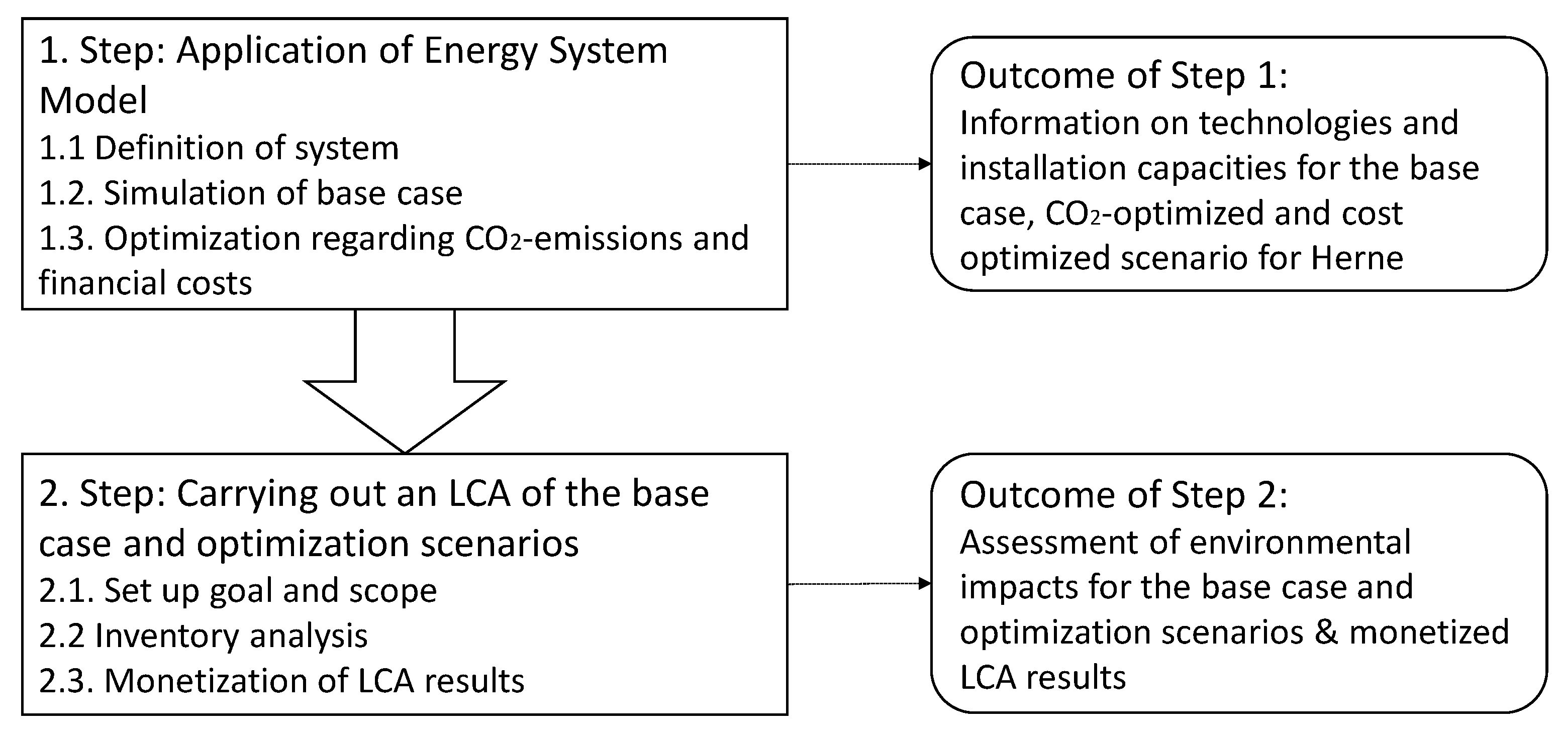
To reach the goals of the paper, steps 1 and 2, as shown in Figure 1, were carried out. The approach was divided into two steps: in step 1 the ESM was applied, to determine the technologies and installed capacities for Herne for the base case and two optimized scenarios, respectively. These scenarios were modelled using the ESM and were used to define the scope of the LCA, which was carried out in step 2. Important output parameters from step 1, in order to be able to perform the LCA, were information on assembly of technologies and their installation capacities. Due to the lack of software for automatic transfer of inputs and outputs, the relevant parameters were transferred manually. Both methods quantify greenhouse gas emissions. The resulting greenhouse gas emissions of both steps were compared at the end, to provide a better basis for decision-making. The steps are explained in more detail in the following subchapters.
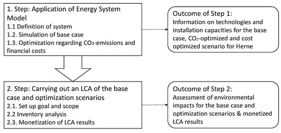
Figure 1.
Step 1 and 2 of the integrated LCA, to analyze the power and heat supply for neighborhoods, using the example of the city Herne in Germany for the base case and two optimized scenarios, including the outcomes of the steps.
2.1. Application of an Energy System Model
First, the system to which the ESM was applied was defined (step 1.1). In order to be able to solve the model with the available computing resources (computing time and memory), the area should contain less than 10 residential and commercial buildings. In addition, the area must be representative and, therefore, be surrounded by streets, contain buildings of various usage types, as well as street and traffic lights.
Next, the base case, referring to the current situation in Herne, was simulated, followed by determining the CO2 and cost optimized scenarios. For the modelling, the energy system model generator (SESMG) by Klemm et al. [17] based on the “Open Energy Modelling Framework” [37,38] was applied. The SESMG uses a bottom-up analytical approach, methods of simulation and optimization, and the mathematical approach of linear optimization. The applied model furthermore considered a building-sharp spatial resolution, a 1-h temporal resolution, and a 1-year time horizon. The underlying Open Energy Modelling Framework (oemof) and its sub-modules were subject to extensive automated testing and validation of infrastructure [37], guaranteeing the functionality of the modelling. The model structure and all input data are documented in detail in Budde [39]. For easier readability, we use SESMG and ESM synonymously; therefore, the applied energy system model will be abbreviated from now on as ESM.
First, the base case of Herne was simulated (step 1.2). The annual electricity and heating demand was estimated based on the building type, building area, number of floors, and number of occupants. The electrical load profile was calculated using the “Richardson tool” [40], whereas the heat demand was calculated based on standard load profiles [41]. Photovoltaic systems were simulated based on weather data from the German Weather Service [42]. The year 2012, an average solar year [43], was chosen as a reference.
As only a small amount of information about heated floors or the state of renovation of the considered houses was provided, the energy demand of the neighborhood was assumed based on existing statistics (e.g., [44,45]). Furthermore, it was assumed that the heat supply was provided by natural gas heating systems and the electricity supply (apart from a photovoltaic system on one of the buildings) by electricity imports from the public distribution grid [44,45].
Next, the CO2 and cost optimized scenarios were simulated (step 1.3), by including additional technologies (e.g., photovoltaic systems), measures (e.g., local electricity exchange), and operation modes (e.g., injection and withdrawal of battery storages), which can potentially reduce the financial costs or CO2 emissions of the system. Then, the combination of technologies, measures, and operation modes for each scenario were defined, minimizing the defined optimization criteria in two separate runs.
The outcomes of step 1 were information on the technologies and installed capacities for the base case, as well as the two scenarios (CO2-optimized and costs optimized), for Herne.
2.2. Carrying Out the Life Cycle Assessment
Next, the LCA was carried out (step 2). Thus, first the goal and scope was defined based on the models derived in step 1 (step 2.1). The goal of the case study was to determine and compare potential environmental impacts for the base case, as well as the two optimized scenarios. The so-called functional unit (FU), quantification of the function of the studied system (here: a neighborhood in Herne), was defined as “the energy supply of electricity and heat to cover the energy demand of the neighborhood for one year”. All flows, as well as the results, are related to the FU. The scenarios differ in their composition of energy supply technologies. They, thus, have varying reference flows (for further information regarding each scenario see Supplement S1, Figures S2–S4).
To ensure comparability between the base case and the scenarios we used the territorial LCA approach Type A, as defined by Loiseau et al. [46]. Furthermore, the following assumptions were made: when more electricity is produced than the district uses, the environmental burdens are still assigned to the district. The effect of this assumption was evaluated in the sensitivity analysis. Additional, surplus electricity from the PV system produced in the territory was modeled as remaining in the neighborhood, according to the territorial approach by Loiseau et al. [46]. Technologies that are the same in all scenarios (e.g., the radiators in the individual buildings) were neglected, as they had no influence on the comparison. Therefore, the focus was on the comparison between scenarios, considering a variety of different impact categories. Material flows such as water, wastewater, building materials, and waste were not considered. See also Supplement S2 for further information regarding assumptions.
We used ReCiPe 2016 (H-hierarchic perspective, midpoint, and endpoint) [47] as an impact assessment method, considering the impact categories of freshwater eutrophication, marine eutrophication, particulate matter formation, fresh water ecotoxicity, human toxicity, ionizing radiation, climate change, land use, stratospheric ozone depletion, photochemical ozone formation, marine ecotoxicity, terrestrial ecotoxicity, terrestrial acidification, metal depletion, fossil resource depletion, and water depletion. The hierarchical perspective corresponds to the standard perspective of the ReCiPe method and weights short- and long-term impacts equally. With ReCiPe, midpoint, as well as endpoint, results for the considered categories can be determined. Midpoint characterization is more closely related to environmental flows, whereas endpoint characterization is easier to interpret, but is subject to greater uncertainty [48]. The midpoint LCA-results were weighted using ReCiPe, according to damage, and can be combined into three endpoint results for human health, ecosystem quality, and resource scarcity [49]. The damage to human health is expressed in DALYs (Disability Adjusted Life Years), where one DALY represents the loss of the equivalent of one year of full health [50]. The damage to ecosystem quality is defined as local relative species loss over space and time. The third category of damage represents the additional financial costs for the future extraction of metal and fossil resources in units of dollars [49].
In the next step (2.2), an inventory analysis was carried out, in which all the processes and their inputs (e.g., resources, water, land) and outputs (e.g., emissions, products), which are needed for the production of a product over its life cycle, are collected and modelled. In this study, we considered all life cycle stages from production till deconstruction or recycling, also referred to as “cradle-to-grave”.
The LCA software GaBi (version 9.1.0.53) by sphera was used for modelling [40]. This software makes it possible to map the entire life cycle of individual technologies and simultaneously calculates the potential environmental impacts of each life cycle stage. For LCI databases GaBi (version 9.1) as well as ecoinvent (version 3.7) were used [51,52]. Values that were not available in either of the two databases were obtained from the literature. If no values were available in the literature, estimates and queries from the industry were used.
The input parameters were derived from the ESM and comprise different energy supply technologies that meet the demand of the neighborhood. Table 1 shows the used technologies and their lifetime, as well as additional data on parts (see also Supplement S2 for further information on the LCI, e.g., transport distances, as well as the used processes of GaBi and ecoinvent for the model).

Table 1.
Overview of considered technologies, their lifetime, and considered LCA stage.
After determining the LCA results, in step 2.3 the LCA results were monetized, which is explained in more detail in the following. The monetary valuation should help to better depict the damage caused to society by environmental impacts, but also which impact category or which damage endpoint is most affected by the assessed technologies. Monetization of environmental impacts indicates the loss of economic welfare that is caused by environmental emissions (per kilogram of the pollutant that is released into the environment) or resource use (used in a certain amount). The prices are expressed in kilograms per emission. Damage becomes visible, for example, through increased health expenses or crop losses [62]. The monetization approach was based on the review by Arendt et al. [63] and is close to the approach used in Arendt et al. [64].
For the monetary valuation of DALYs, the European Commission’s guideline on the monetary valuation of QALY (Quality Adjusted Life Years) was used [65]. Here, QALY is effectively the positive value of a DALY and does not express the loss of a year of full health, but values years of life in perfect health with a factor of 1.0, while years in less perfect health are valued with a lower factor. QALYs are valued at a minimum of 50,000 €2009 to a maximum of 80,000 €2009 per QALY in the European Commission’s guideline and are applied analogously to the valuation of DALYs in this paper. For the monetary valuation, the prices were inflation-adjusted with the help of the consumer price index and adjusted to the year 2020. If necessary, the currencies were converted with purchasing power parities.
The assessment of resource scarcity has already been issued as a monetary result (unit $2003) and was therefore first adjusted for inflation and converted into Euro (€2020). The result should be understood as future financial costs for future extraction of an additional unit of material [49].
The damage to an ecosystem is difficult to assess in monetary terms. To be able to carry out a monetary valuation nevertheless, the monetary value of Kuik et al. [66] was used. The average terrestrial species density was determined to be 1.48 × 10⁻⁸ species/m2 and 0.69 €2020/PDF/m2/yr. PDF stands for the potentially disappeared fraction and can be equated with species in this formula [49,62]. We used the highest value terrestrial species density for terrestrial as well as seawater ecosystems, because seawater ecosystems are more likely to be generally underestimated [67].
3. Results
In the following, the results are presented. First, the results of the base case and the two optimized scenarios (Section 3.1) are introduced. Then, the results of the normalized LCA are presented at mid-point level and on end-point level (3.2). Last, the monetized results (3.3) are shown.
By comparing the results of both modelling approaches, we could provide insights into the importance of a joint approach of EMS and LCA. With the detailed LCA of each scenario, it is easy to identify which burden shifts will occur by changing existing energy generation strategies. It is also possible to determine the technology or the process that leads to the highest burden. Combining the information helps to analyze the relationship between impact categories and technology. Therefore, the EMS can be adjusted and can provide detailed information for the decision-making process.
3.1. Derived Base Case and Scenarios for Herne Based on ESM Modelling
The ESM modelling provided the necessary information such as energy consumption, technology composition, and installed capacities in each scenario, for the base case and considered scenarios. An overview of the electric and heat energy is given in Table 2.
Table 2.
Supply of heat and electricity for the different scenarios.
In the base case, supply of heat (629,432 kWh/year) is provided by gas boilers in each building. The supplied electricity (132,210 kWh/year) is generated by the public grid for each building and additionally a PV-system for the commercial building.
The optimized scenarios show how the optimization criterion could be minimized in the investigated period. This includes the selection of the most suitable technologies (e.g., battery storage), as well as their capacities and the ideal modes of operation (e.g., when to store and retrieve the battery storage) of the technologies used. Due to the linear optimization approach, this may result in capacities that do not necessarily correspond to plants available on the market.
In the CO2-optimized scenario the supply of heat (629,432 kWh/year) is provided by a local heat network in combination with one CHP, by using natural gas from the public grid and one surface water heat pump (SWHP). The supply of electricity (260,778 kWh/year) is provided by CHP, PV-systems on all buildings and battery storage systems.
In the cost-optimized scenario the supply of heat (629,432 kWh/year) is generated by gas boilers, as well as five ground coupled heat pumps (GCHP), one in each building. The electricity (236,740.15 kWh/year) is supplied by the public grid for each building and additionally by PV systems on all buildings.
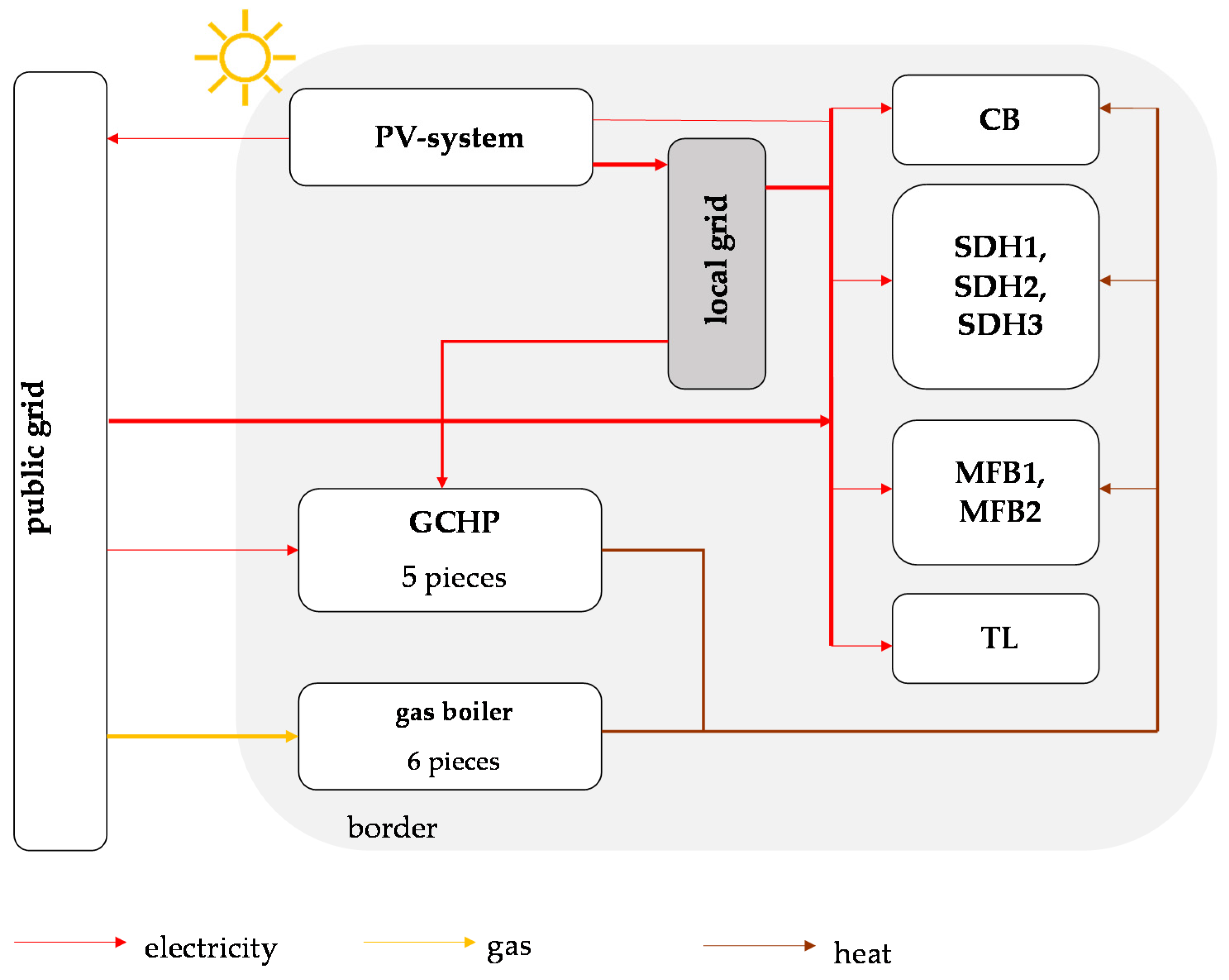
Figure 2, shows the distribution of energy flows in the considered area for the cost-optimized scenario.
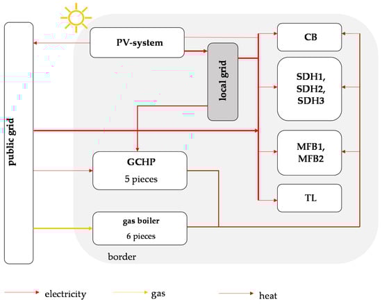
Figure 2.
Overview of the cost-optimized scenario of the neighborhood under consideration. The grey area delimits the observation area. The relevant technologies for electricity and heat supply are shown. The directions of the arrows show the flow direction. The local grid symbolizes the electricity exchange between buildings. The abbreviations stand for the individual buildings: Semi-detached house (SDH), commercial building (CB), multi-family building (MFB), traffic lights and streetlights (TL). The individual buildings are each supplied by a gas boiler and by a GCHP (ground coupled heat pump). Compared to the CO2-optimized scenario, there is no heating network in the neighborhood.
The local grid provides electricity to cover the remaining demand for heating (via a heat pump) and consumption. The distribution between consumers is ensured by a local grid inside the area. The installed PV-systems on each building generate electricity for the building, and surplus energy is provided for other consuming units inside the area (e.g., traffic lights or other buildings). The remaining electricity is fed into the public grid.
An overview of the technologies used in the individual scenarios can be found in the Supplement S1, Figures S2–S4.
3.2. LCA Results at Midpoint Level and Endpoint-Level
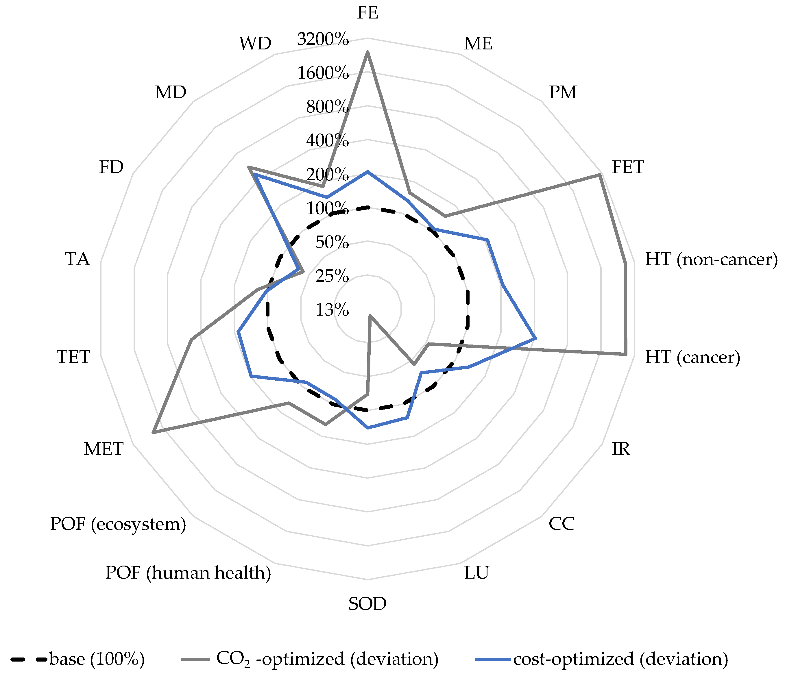
The relative LCA results of the base case compared to the two scenarios are shown in Figure 3. The base case is defined as 100%, whereas the other two scenarios are shown as a percentage deviation from the base case. The axis is logarithmic, for better representability.

Figure 3.
Percentage deviation of the two target scenarios from the base scenario. The base scenario is used as the reference scenario in the presentation and the adverse effect is defined as 100% in each category. For the target scenarios, the changes in the environmental impact categories are each calculated referring to the reference scenario and presented as percentage deviations from the actual scenario. Values greater than 100% represent a greater environmental impact, smaller values a lesser environmental impact. For better representation, the axis is logarithmic. Abbreviations: FE = freshwater eutrophication, ME = marine eutrophication, PM = particulate matter formation, FET = fresh water ecotoxicity, HT = human toxicity, IR = ionizing radiation, CC = climate change, LU = land use, SOD = stratospheric ozone depletion, POF = photochemical ozone formation, MET = marine ecotoxicity, TET = terrestrial ecotoxicity, TA = terrestrial acidification, FD = fossil depletion, MD = metal depletion, and WD = water depletion.
While the environmental impacts of the categories climate change and terrestrial acidification are reduced within both scenarios, the environmental impacts of ecotoxicity, human toxicity, and eutrophication increase significantly. Especially in the CO2-optimized scenario, the battery storage influences the results. For example, human toxicity is 30-times higher in the CO2-optimized scenario than in the base case, but only 14-times higher in the cost-optimized scenario, which is largely due to the battery storage. In addition, particulate matter formation almost doubles in the CO2-optimized scenario, and marine ecotoxicity is 19-times higher than in the base case. In the cost-optimized scenario, greenhouse gas emissions are slightly lower than in the base case, while in the CO2-optimized scenario, they are reduced by almost 50%. The impact on land use is the lowest in the CO2-optimized scenario, because no electricity from the public grid is used, which leads to high land use impacts. As the used methods to assess human and eco toxicity in ReCiPe are subject to uncertainty [68,69], in the following, the focus is on the selected impact categories (categories climate change (CC), land use (LU), mineral depletion (MD), and photochemical ozone depletion (POF)). Sometimes we refer to other impact categories, which are not shown in the following figures, and these can be found in the Supplement S1, as well as an overview on all results.
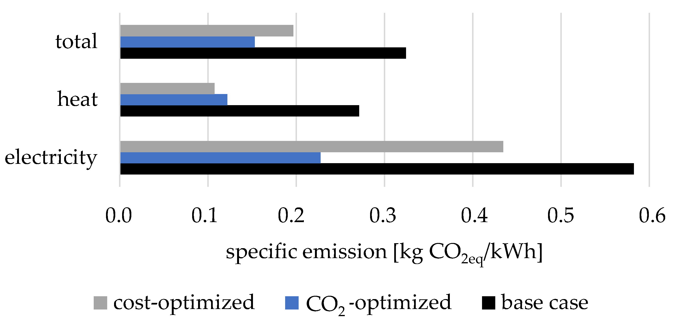
In each scenario, the heat demand is 629,432 kWh/year. The heat pumps increase the electricity demand in the two optimized scenarios from 132,210 kWh/year (base case) to 260,778 kWh/year (CO2-optimized) and 236,740 kWh (cost-optimized). For the climate change potential of each scenario, specific CO2eq per kWh were determined (see Figure 4).

Figure 4.
Overview on the specific emissions for each scenario in kg CO2eq/kWh, without accounting for emissions with energy-related infrastructure. A distinction is made between the joint consideration of heat and electricity (=total) in kg CO2eq/kWh and electricity and heat separately.
While the cost-optimized scenario shows a small reduction in specific emissions in electricity supply, the specific emissions for heat supply are even lower than those of the CO2-optimized scenario. A comparison of the cost-optimized scenario with the base case scenario shows a reduction in the specific emission factor of almost 40%, and more than 50% in the CO2-optimized scenario. However, the increased electricity demand of the two target scenarios reduces the amount of CO2eq saved. With the help of the information concerning the neighborhood, we calculated the specific CO2eq per person and year, without accounting for emissions from energy-related infrastructure, such as radiators or power cables. For the base case, the specific CO2eq emissions sum up to 3.23 tons per person each year, for the CO2-optimized scenario to 1.64 tons per person each year, and for the cost-optimized scenario to 1.84 tons per person each year.
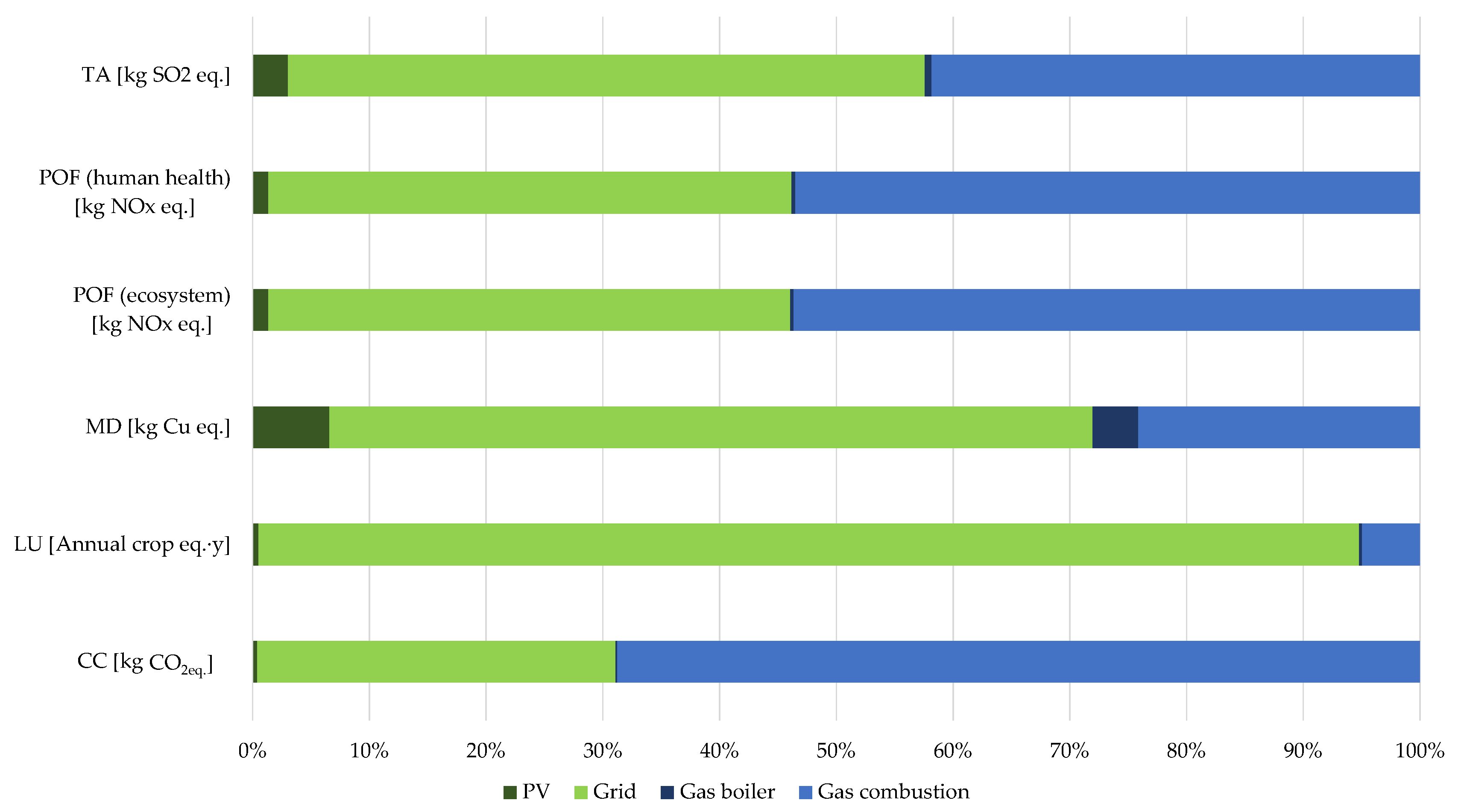
In Figure 5, Figure 6 and Figure 7, the distribution of environmental impacts is explored, showing which impacts occur due to either electricity or heat supply within all three scenarios. The colors of the bars represent the technology affiliation to either electricity supply (green) or heat supply (blue). If a technology provides both heat and electricity, the color orange is used. Figure 5 shows the share of the used technologies and energy sources in the base case scenario.
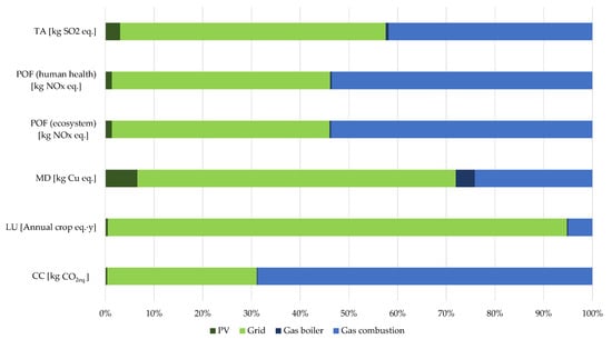
Figure 5.
Results of base case, percentage distribution, midpoint level. Abbreviations: CC = climate change, LU = land use, POF = photochemical ozone formation, TA = terrestrial acidification, MD = metal depletion.

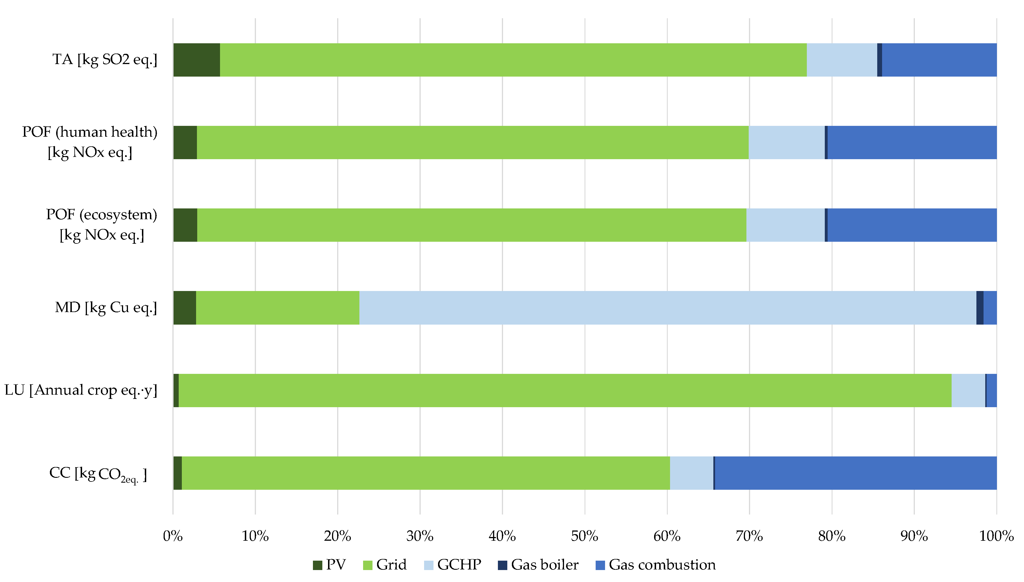
Figure 6.
Results of cost-optimized, percentage distribution, and midpoint level. Abbreviations: CC = climate change, LU = land use, POF = photochemical ozone formation, TA = terrestrial acidification, MD = metal depletion.

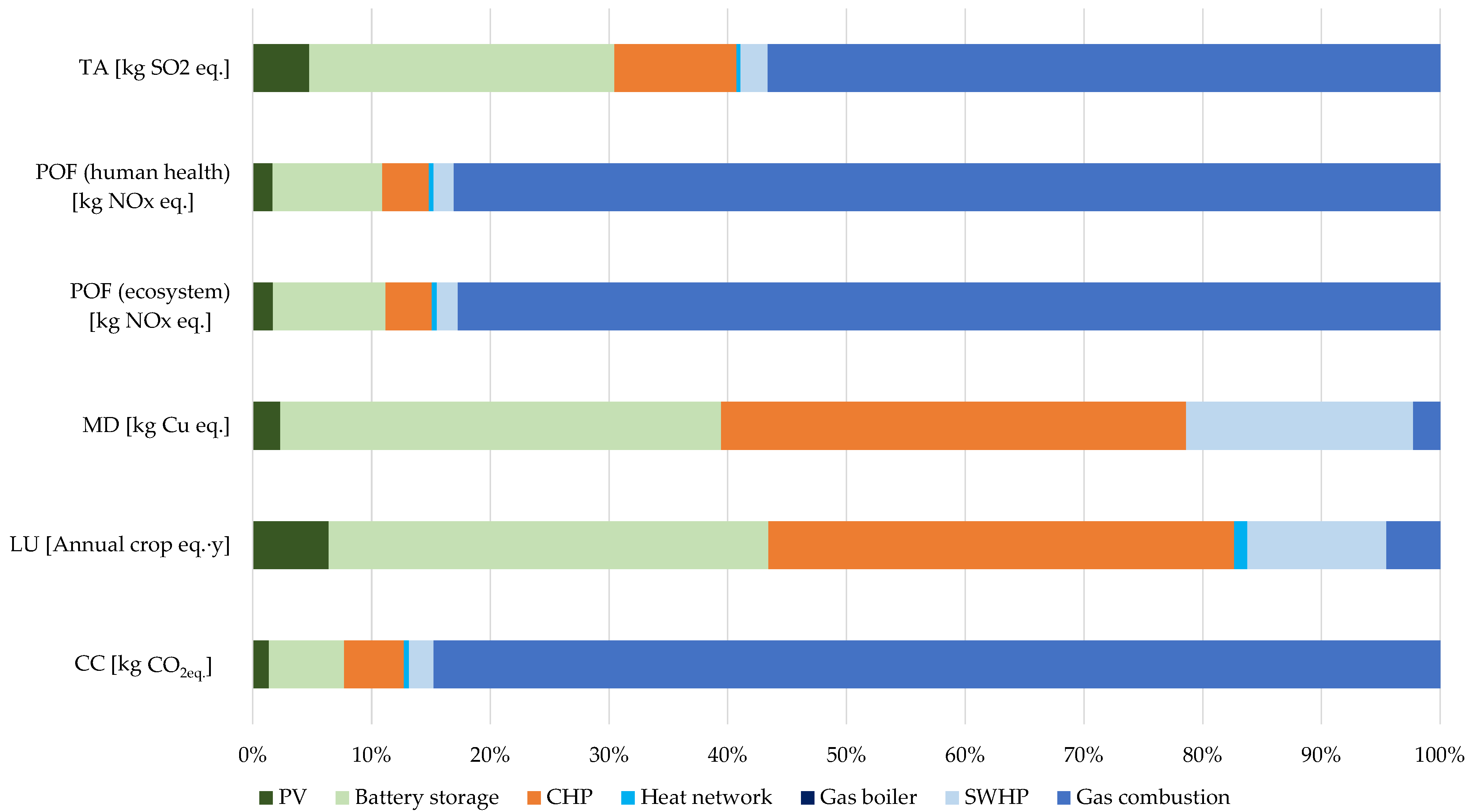
Figure 7.
Results of CO2-optimized, percentage distribution, and midpoint level. Abbreviations: CC = climate change, LU = land use, POF = photochemical ozone formation, TA = terrestrial acidification, MD = metal depletion. 3.3. LCA results at endpoint level.
As energy is almost exclusively supplied by grid electricity and gas combustion, in almost all categories, these dominate the result. Having long lifetimes, the environmental impact due to the production and end-of-life of the technologies is no more than 15% in the mentioned categories. Gas combustion contributes to almost 70% of climate change. Only in the categories freshwater eutrophication, freshwater, and marine ecotoxicity, as well as human toxicity, does the PV system account for the largest share (see Supplement S1 Figures S5–S7). In the case of the PV system, no environmental impacts occur in the operational phase; they only occur during production (e.g., due to cell manufacturing) and EoL (e.g., due to dismantling and recycling/waste management). Having a deeper look into the production of PV systems, the highest share of mineral depletion is caused by the module assembly, which causes a high demand of electricity during production. For the gas boiler, a large part of the environmental impact is caused by the gas combustion in the operational phase, while the production and EoL-phase are less relevant.
Furthermore, the annual CO2eq emissions (approx. 247 t CO2) for the base case are significantly higher as estimated by the EMS simulation (approx. 199 t CO2 per year). The reason for this is presumably the partially different data basis and the more precise consideration of the whole life cycle of all technologies within the LCA.
Figure 6 shows the distribution of the individual technologies and energy sources in the cost-optimized scenario.
It can be seen that the electricity supply contributes more to the environmental impact in the neighborhood than the heat supply. This is due to the increased electricity demand for the area from the heat pump, as less natural gas is needed to cover an equal heating demand compared to the base case. While the gas boilers show hardly any environmental impact in all categories, the GCHP contributes significantly to the environmental impact in some categories. The carcinogenic human toxicity and metal depletion is dominated by the GCHPs. More metals are needed to produce the GCHP than to make a gas boiler. The use of heat pumps shifts the environmental impact toward production and end-of-life processes.
Furthermore, in the cost-optimized scenario, the ESM delivers significantly lower emissions (approx. 130 t CO2 per year) compared to the LCA, with 170 t CO2eq per year. Here, there is a deviation of about 40 t CO2eq per year.
These results show that a consideration of the specific emission factors of electricity (e.g., of PV systems or CHP units) and heat does not lead to a complete representation of the emissions. The deviation is particularly large in the base case and cost-optimized scenario, in which grid electricity is purchased. It would be useful to review which of the specific emission factors considered in the ESM and LCA better reflects reality.
In the CO2-optimized scenario (see Figure 7), the dominant systems are battery storage and gas combustion in the CHP. The CHP contributes strongly to the environmental impact in the categories metal depletion and land use. The contribution of the gas boilers is negligible, as they are only built back in the CO2-optimized scenario and are not needed for heat provision. The heating network hardly contributes to the environmental impact.
In the following, the results on end-point level are presented (see Table 3). A decrease in impacts of human health (DALY) and resources (USD 2003) can be seen in the two optimized scenarios, while the ecosystem (species year) impacts increase. It should be noted however, that, at least for the DALY values, the variation between the scenarios cannot be considered significant, especially for the human health impacts caused by human toxicity [70]. A detailed overview of the distribution at endpoint level can be found in Table S1 (Supplement S1). A high share contribution of the ecosystem damage was caused by the battery storage. Thus, the scenario was calculated with reduced battery storage (half the storage capacity), which significantly reduced the impacts.
Table 3.
ReCiPe endpoint results in each scenario.
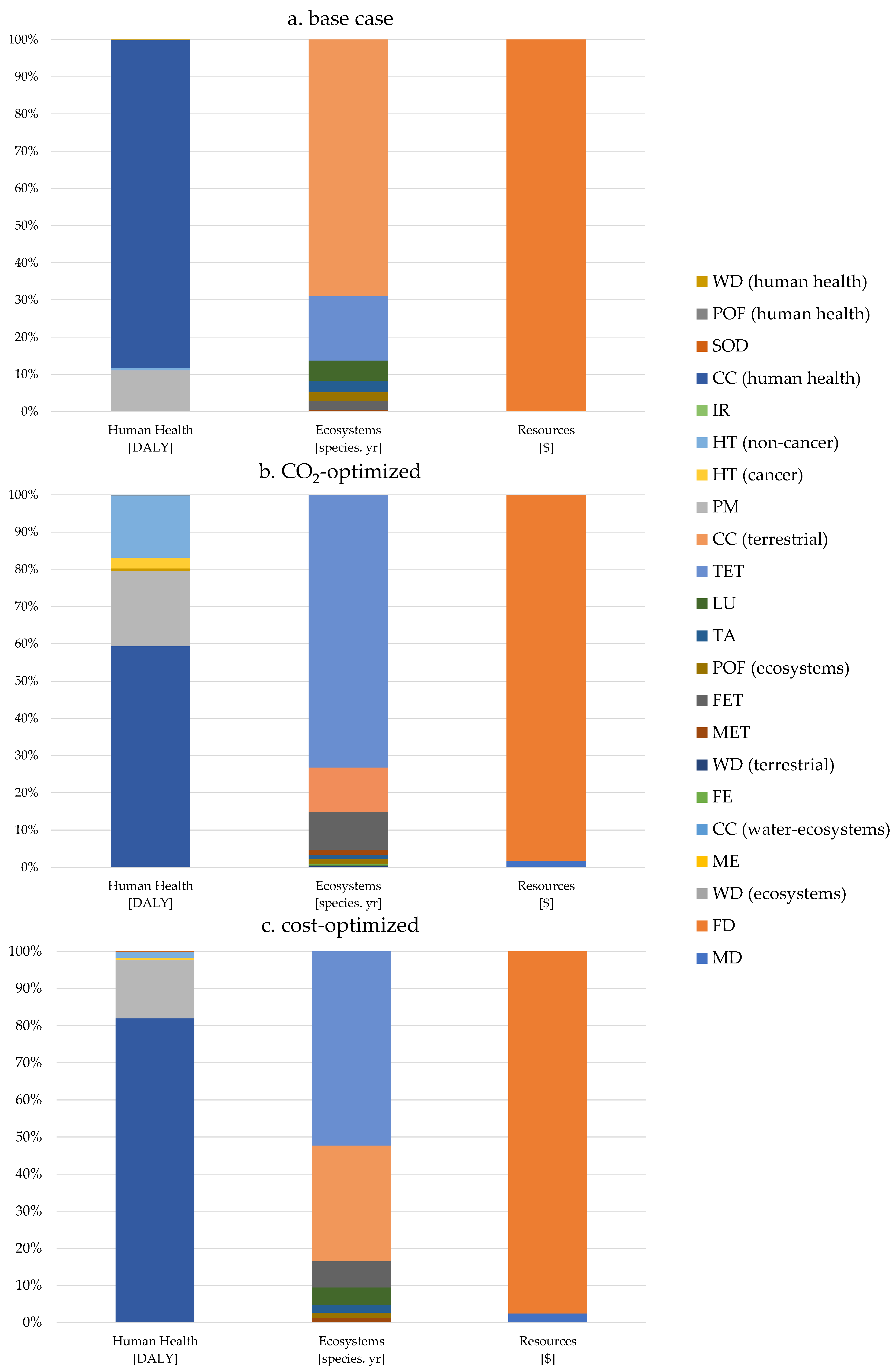
The results of the endpoint assessment are summarized for the three scenarios in percentage distribution, as well as in total distribution, in Figure 8.
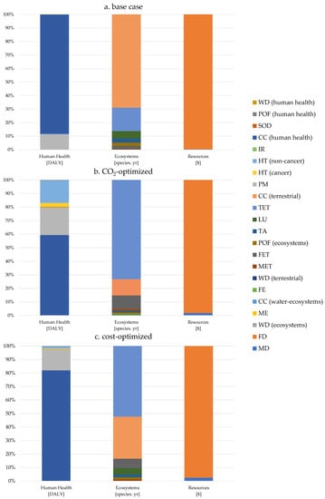
Figure 8.
The figure shows the percentage distribution in each scenario at endpoint level. Up to down: base case, CO2-optimized, cost-optimized. Corresponding impact categories to each endpoint level in the following. Human Health: WD (human health), POF (human health), SOD, CC (human health), IR, HT (non-cancer), HT (cancer), PM | Ecosystems: CC (terrestrial), TET, LU, TA, POF (ecosystems), FET, MET, WD (terrestrial), FE, CC (water-ecosystems), ME, WD (ecosystems)| Resources: FD, MD. Abbreviations: FE = freshwater eutrophication, ME = marine eutrophication, PM = particulate matter formation, FET = fresh water ecotoxicity, HT = human toxicity, IR = ionizing radiation, CC = climate change, LU = land use, SOD = stratospheric ozone depletion, POF = photochemical ozone formation, MET = marine ecotoxicity, TET = terrestrial ecotoxicity, TA = terrestrial acidification, FD = fossil depletion, MD = metal depletion, WD = water depletion.
For the base case, around 99.74% of the impact on the AoP resources is due to the extraction of fossil raw materials and only 0.26% from the depletion of metals. ReCiPe assigns higher externalities to fossil resources, instead of metal depletion [71]. Climate change contributes most to ecosystems and human health for the base case scenario.
In the cost-optimized scenario, the consumption of fossil resources continues to contribute the highest share to the consumption of resources, because, one the one hand, a lot of fossil energy sources are used and, on the other hand, ReCiPe assess their use as relatively high. The greatest damaging effect on the ecosystem or biodiversity in this scenario comes from terrestrial ecotoxicity and, to almost the same extent, from climate change. For human health, climate change and particulate matter remain the highest impacts. For the results of the CO2-optimized scenario, in the base case, the use of fossil resources does not play a role. The ecosystem, however, is not most impacted by climate change, but by terrestrial ecotoxicity. Climate change impacts on terrestrial ecosystems and freshwater ecotoxicity each contribute about 10% of the impact. Human health is particularly affected by climate change and particulate matter, but non-carcinogenic human toxicity also plays a decisive role, accounting for almost 20%. When we compare the three scenarios, it is noticeable that in the categories human toxicity and water depletion, the CO2-optimized scenario has the highest value. For ionizing radiation, on the other hand, it has the smallest. The CO2-optimized scenario reduces the impact in land use, while the impacts on freshwater eutrophication and terrestrial ecotoxicity rise. The damage due to fossil depletion shrinks in both optimized scenarios, the damage due to metal depletion rise.
3.3. Monetization of LCA Endpoint Results
The results of the monetary valuation, which shows the associated damages from the technologies, can be seen in Table 4. This shows higher environmental costs for the ecosystem in both optimized scenarios. Especially in the CO2-optimized scenario, they are about 200% higher than in the base case. This is mainly due to the external effects of toxicity that might affect ecosystems. For human health and resource consumption the environmental costs are reduced.
Table 4.
Monetary valuation of endpoint-results in the three scenarios in EUR for 2020. The percentage deviation from the actual scenario is shown in brackets.
With a reduction of battery storage capacity (which was dimensioned with a high capacity in the ESM) the environmental impacts in the impact category terrestrial ecotoxicity could be reduced by over EUR 50,000 in externalities. This would lead to a significantly smaller damage to ecosystems. The damages are, however, still higher than the damages in the base case. However, the damages are mostly related to the impact category terrestrial ecotoxicity. Not considering this category would decrease the total damages of the CO2-optimized scenario to the lowest costs (EUR 54,000). The toxicity impacts mostly stem from printed circuit boards and printed wring board production. However, this trade-off should be interpreted with caution, as toxicity impacts have a high uncertainty. Furthermore, the electricity production in the CO2-optimized scenario and the cost-optimized scenario are higher than those in the base case, as visible in Table 1, which is discussed in the sensitivity analysis (see Section 4.4).
4. Discussion
In the following, first, the underlying inputs of the ESM are discussed regarding their plausibility (Section 4.1), followed by an evaluation of the transferability of the approach to other neighborhoods (Section 4.2). Next, the limitations and assumptions of the LCA results are analyzed (Section 4.3), followed by a sensitivity analysis (Section 4.4).
4.1. Assessment of Input Parameters
The input parameters of the LCA are strongly dependent on the results of the ESM. The ESM model provides information on the considered technologies and the generation capacity of the individual technologies. The modification of the following parameters might improve the model:
- The supplementation of CHP units with peak load boilers could possibly lead to a reduction of the required CHP capacity, while further minimizing the optimization criteria.
- The switch of the nearby district heating power plant in Herne, from coal to gas [72], could have a significant impact on the connection decision. Generally, changes of technology (e.g., technological development in the hydrogen sector) could have significant effects on the model outcome, as this depends on the cost and CO2-intensity of the technologies.
- In the development of neighborhoods, changes regarding the energy demand of households should be considered. For example, the electrification of transport alone is expected to increase the demand for electricity. For long-term optimization, it is therefore advisable to model different demand scenarios and to optimize them. In this context, decreasing energy demand should also be considered, for example due to improved building insulation.
- As the city of Herne does not assess greenhouse gas emissions by district, but only at city level, the results cannot be validated against other results that were calculated by the communal government. Such a validation would be desirable.
4.2. Transferability of the Modelling to Larger Neighborhoods and Recommendations for Further Research
The energy supply scenarios determined by the ESM were modelled using LCA. The recommended technology compositions for the neighborhood and the corresponding generation capacity of the individual technologies serve as input parameters for the LCA and are fixed. The results can be easily applied and scaled to neighborhoods with the same technology composition. For this, only the consumption, generation capacity, and output of the technologies are required. All relevant data can be determined using the conversions mentioned in this paper. For similar neighborhoods, in terms of final energy demand, the modelling of the current state will be sufficiently accurate; however, the optimized scenarios can vary greatly due to local conditions. For example, a nearby body of water is a requirement for the use of a SWHP. For larger neighborhoods, ESM might recommend a different energy supply mix, in which case the results of the LCA cannot be applied in the modelling, without major adjustments. Generally, PV modules are often recommended in the model. However, the optimal technology mix depends on local conditions and will not be the same for every German settlement structure.
Comparing the results of the modelled base case with the officially published CO2 emissions per capita from the city Herne for 2010 showed that the official statistics are, at 4.2 t CO2/capita, slightly below our results (without transport) [73]. Deviations might occur due to our assumptions on heating and electricity demand because of missing data.
We recommend that the results of the energy system model presented here should be validated as soon as studies on the energy system greenhouse gas emissions of individual neighborhoods are available for the municipality of Herne. Furthermore, the battery storage should be revised to reduce the burden shift to other impact categories.
Future research should integrate more technologies into ESM, giving more detailed results for the optimization of neighborhoods. Additionally, the added technologies need to be assessed in an LCA, to complement these results and to provide more detailed profiles of their environmental impacts.
Currently, political and economic developments (e.g., increase in gas price or CO2 price) in the energy market are not taken into account in the model. These changes could play a major role in optimization, especially in terms of costs, and should be integrated. In the next step, a single software solution for the combination of ESM and LCA would be desirable. Providing a single software would simplify the application for additional users. A challenge for this will be proprietary data, especially for the application of the LCA.
4.3. Assessment of Limitations and Assumptions of the LCA
In the following, the limitations and assumptions of the LCA are described. One difficulty of modelling is the available data basis, especially for the end-of-life modelling of the CHP, PV, and battery storage systems. Many of the published studies do not consider the end-of-life of battery storage and PV systems. PV systems for residential use have only begun to emerge in recent decades. Currently, reliable end-of-life data are missing, because the first PV systems in Germany will only come off the EEG (renewable energy law) subsidy in 2020, and with long lifespans of 20 to 25 years, the problem of recycling is still to come. Furthermore, battery storage systems have only recently become economically viable for home applications. Thus, no final recycling method has been established yet. The guidelines implemented in Germany are intended to ensure that the materials are returned to the cycle in the long term.
Simplified linear relationships have been used for the scaling of the technologies. Not every technology is available in all performance sizes, rather there are performance classes which require certain technologies to be modeled in a larger performance class. This may entail a higher consumption of resources.. For example, linear scaling is appropriate for the heat grid and PV modules, while a different scaling factor would be more appropriate for the inverter [74,75]. The inverter had significant impacts on the toxicity impacts and therefore the linear scaling assumption should be verified in additional studies. Compared to gas combustion and grid procurement, the considered technologies hardly contributed to the environmental impacts of the respective scenarios, except for the battery storage, which dominated almost all environmental impact categories in the CO2-optimized scenario. Here, it must be examined to what extent another scaling factor would be more appropriate and whether the limiting parameters of ESM are appropriate for certain technologies.
4.4. Sensitivity Analysis
The influence of various assumptions was modelled and shown in a sensitivity analysis. The greatest influence was a reduction in the capacity of the battery storage. The modelling of the surplus energy, either to stay inside the modelling area, or to be accounted as a credit for feed-in surplus of energy into the grid was assessed. The effect of a refrigerant without GWP was also considered, other changes can be found in Supplement S3.
A territorial LCA Type A was applied, where the surplus of electricity was modelled to be consumed inside the neighborhood. To obtain a better understanding of the change of environmental impacts, a credit in the form of a reduction in environmental impacts for the feed-in surplus of solar energy, with the help of the future German electricity mix of 2030, instead of being consumed inside the neighborhood, was modelled. In the base case this reduced the environmental impact, especially in the categories of water consumption (−20%) and land use (−66%), while the environmental impact of the energy supply in the neighborhood would increase in the categories of terrestrial ecotoxicity (+22%) and carcinogenic human toxicity (+8%). In the cost-optimized scenario, around approx. 44,670 kWh are credited with the forecast German electricity mix for 2030, reducing the environmental impact of the energy supply by approx. 22% in each of the areas of land use and seawater eutrophication. A decrease in environmental impact can also be observed in the categories climate change (−13%), ozone depletion (−17%), and consumption of fresh water (−15%), among others. Due to the large battery storage systems in the CO2-optimized scenario, almost no surplus of electricity is fed into the grid; therefore, no relevant reduction in the environmental impact of the scenario is obtained.
The influence of refrigerants in the heat pump in both optimized scenarios was analyzed by modelling refrigerants without a greenhouse gas effect in the sensitivity analysis. In the CO2-optimized scenario, they reduced the environmental impact of the energy scenario in terrestrial ecotoxicity by almost 20%; ozone depletion and carcinogenic human toxicity were each reduced by approx. 15%; and the consumption of metals and land use were each reduced by 35%. In the other environmental impact categories, only a slight change can be observed (up to–9%). In the cost-optimized scenario, the impact was only significant in the categories of terrestrial ecotoxicity (−30%), ozone depletion (−21%), consumption of metals (−13%), and seawater ecotoxicity (−11%).
It was assumed that the battery storage with a total of 617 kWh available capacity are only supplied by the surplus electricity from the PV systems and provide the neighborhood with approx. 43,336 kWh, distributed over a year (Note: the proportion of electricity from the CHP stored in the battery storage was neglected). Considering the specific CO2eq of one kWh of PV electricity, approx. 204 g CO2eq/kWh are produced for a kWh of electricity from the battery storage. If electricity from the CHP is also stored, the specific emission factor deteriorates accordingly. For a sensible dimensioning of the battery storage, a storage capacity of 1 kWh per kW of the PV system peak capacity is recommended. In this case, an increase in self-sufficiency can no longer be expected with more than 2 kWh per kW of the PV systems peak capacity [76]. In this scenario, there are just under 9 kWh of storage capacity per kW of PV system peak capacity. To model the influence of a smaller storage system, the storage capacity was reduced to approx. 70 kWh. This reduced marine and freshwater ecotoxicity and eutrophication by more than 80%, and human toxicity by approx. 83% (carcinogenic) and by 69% (non-carcinogenic). In contrast, a reduction in battery storage had hardly any influence on the specific CO2eq emissions of the energy supply (−5.6%), photochemical ozone formation (−8%) and the depletion of fossils (−5.5%). This reduced dimensioning of the battery storage is likely to resolve the trade-off between climate change and toxicity.
5. Conclusions
In this study, an integrated LCA was implemented by combining LCA and ESM. This allowed the consideration of additional environmental impacts beyond greenhouse gas emissions and provided deeper insights into the implementation of new technologies.
In the base case, heat was supplied by gas boilers and grid electricity. These technologies were substituted with CHPs, surface water heat pumps, and PV-systems in the CO2-optimized scenario. Five ground coupled heat pumps and PV-systems provide energy and heat for the cost-optimized scenario. These technology shifts could reduce greenhouse gas emissions by 40% in the cost optimized and more than 50% in the CO2-optimized scenario. However, these technologies do not leave the other impact categories unaffected. For example, oversized battery storage risks increased impacts in other categories such as terrestrial eco toxicity, by around 22%. Additionally, using the ESM without LCA might lead to an underestimation of greenhouse gas emissions of around 10%. Thus, it can be recommended to use smaller battery storage systems to avoid burden shifts to other impact categories. Through the combination of ESM and LCA, decision-makers can rely on more detailed data of environmental impacts when they revise the energy supply of an existing neighborhood.
Supplementary Materials
The following supporting information can be downloaded at: https://www.mdpi.com/article/10.3390/en15165900/s1. Figure S1: Overview over the considered area in Herne, Germany. G = Garage, SDH = semi-detached house, TL = Traffic lights and streetlights, MFB = multiple family building, CB = commercial building. (source: google maps); Figure S2: Overview of the current state of the neighborhood under consideration. The relevant technologies for electricity and heat supply are shown. The directions of the arrows stand for the flow direction. The abbreviations stand for the individual buildings: Semi-detached house (SDH), commercial building (CB), multiple family building (MFB), traffic lights and streetlights (TL).; Figure S3: Overview of the emission-optimized scenario of the neighborhood under consideration. The relevant technologies for electricity and heat supply are shown. The directions of the arrows stand for the flow direction. The abbreviations stand for the individual buildings: Semi-detached house (SDH), commercial building (CB), multiple family building (MFB), traffic lights and streetlights (TL). The gas boilers already present in the neighborhood will be dismantled.; Figure S4: Overview of the cost-optimized scenario of the neighborhood under consideration. The relevant technologies for electricity and heat supply are shown. The directions of the arrows stand for the flow direction. The abbreviations stand for the individual buildings: Semi-detached house (SDH), commercial building (CB), multi-family building (MFB), traffic lights and streetlights (TL). The individual buildings are each supplied by a gas boiler and by a GCHP. Compared to the CO2-optimized scenario, there is no heating network in the neighborhood.; Figure S5: base case, percentage distribution, midpoint level; Figure S6: cost-optimized, percentage distribution, midpoint level; Figure S7: CO2-optimized, percentage distribution, midpoint level; Table S1: Total result on endpoint level per impact category; Supplements S2: Additional Information (LCI); Supplements S3: Additional Information on Sensitivity Analysis.
Author Contributions
Conceptualization, G.Q., C.K., R.A., V.B. and P.V.; Data curation, G.Q., C.K. and J.B.; Funding acquisition, P.V. and M.F.; Methodology, G.Q. and C.K.; Project administration, R.A., V.B., P.V. and M.F.; Software, C.K. and J.B.; Supervision, R.A., C.K., V.B. and M.F.; Validation, G.Q., J.B., C.K. and R.A.; Visualization, G.Q. and R.A.; Writing—original draft, G.Q.; Writing—review & editing, R.A., C.K., V.B., P.V. and M.F. All authors have read and agreed to the published version of the manuscript.
Funding
This research was conducted within the R2Q project, funded by the German Federal Ministry of Education and Research (BMBF)-grant number 033W102E and 033W102A.
Institutional Review Board Statement
Not applicable.
Informed Consent Statement
Not applicable.
Acknowledgments
We acknowledge support by the German Research Foundation and the Open Access Publication Fund of the TU Berlin.
Conflicts of Interest
The authors declare no conflict of interest.
References
- Statista Prognose zur Entwicklung der Weltbevölkerung bis 2100. Available online: https://de.statista.com/statistik/daten/studie/1717/umfrage/prognose-zur-entwicklung-der-weltbevoelkerung/ (accessed on 7 August 2020).
- United Nations-Department of Economic and Social Affairs Population Division. World Urbanization Prospects: 2018: Highlights; United Nations Environment Programme: Nairobi, Kenya, 2019; ISBN 978-92-1-148318-5. [Google Scholar]
- Rode, P.; Burdett, R. Cities: Investing in Energy and Resource Efficiency. In Towards a Green Economy: Pathway to Sustainable Development and Poverty Eradication; United Nations Environment Programme: Nairobi, Kenya, 2011; pp. 453–492. [Google Scholar]
- United Nations Cities: A “Cause of and Solution to” Climate Change. Available online: https://news.un.org/en/story/2019/09/1046662 (accessed on 26 January 2022).
- United Nations Human Settlements Programme. The Value of Sustainable Urbanization-World Cities Report 2020; United Nations Human Settlements Programme, Ed.; United Nations Human Settlements Programme: Nairobi, Kenya, 2020. [Google Scholar]
- GERICS. Cities and Climate Change - Climate-Focus-Paper; GERICS, Ed.; Climate Service Center Germany: Hamburg, Germany, 2015. [Google Scholar]
- SDG Goal 11: Sustainable Cities and Communities. Available online: https://www.globalgoals.org/11-sustainable-cities-and-communities (accessed on 26 January 2022).
- Europäische Kommission Übereinkommen von Paris. Available online: https://ec.europa.eu/clima/policies/international/negotiations/paris_de (accessed on 7 August 2020).
- ICLEI GreenClimateCities Programm. Available online: https://iclei.org/en/GreenClimateCities.html (accessed on 29 September 2021).
- Salvia, M.; Reckien, D.; Pietrapertosa, F.; Eckersley, P.; Spyridaki, N.-A.; Krook-Riekkola, A.; Olazabal, M.; De Gregorio Hurtado, S.; Simoes, S.G.; Geneletti, D.; et al. Will Climate Mitigation Ambitions Lead to Carbon Neutrality? An Analysis of the Local-Level Plans of 327 Cities in the EU. Renew. Sustain. Energy Rev. 2021, 135, 110253. [Google Scholar] [CrossRef]
- Reckien, D.; Salvia, M.; Heidrich, O.; Church, J.M.; Pietrapertosa, F.; De Gregorio-Hurtado, S.; D’Alonzo, V.; Foley, A.; Simoes, S.G.; Krkoška Lorencová, E.; et al. How Are Cities Planning to Respond to Climate Change? Assessment of Local Climate Plans from 885 Cities in the EU-28. J. Clean. Prod. 2018, 191, 207–219. [Google Scholar] [CrossRef]
- IEA. Market Report Series: Renewables 2018–Analysis; International Energy Agency: Paris, France, 2018. [Google Scholar]
- BMWi. Klimaschutzplan 2050; BMWi: Berlin, Germany, 2022. [Google Scholar]
- REN21. Renewables 2019 Global Status Report; REN21: Paris, France, 2019; ISBN 978-3-9818911-7-1. [Google Scholar]
- BDEW. Wie Heizt Deutschland 2019? BDEW-Studie Zum Heizungsmarkt; BDEW: Berlin, Germany, 2019. [Google Scholar]
- Umweltbundesamt Energieverbrauch für Fossile und Erneuerbare Wärme. Available online: https://www.umweltbundesamt.de/daten/energie/energieverbrauch-fuer-fossile-erneuerbare-waerme (accessed on 14 September 2020).
- Klemm, C.; Budde, J.; Wittor, Y.; Vennemann, P. Spreadsheet Energy Model Generator (GIT): SESMG. Available online: https://spreadsheet-energy-system-model-generator.readthedocs.io/en/latest/. (accessed on 7 June 2021).
- Hertwich, E.G.; Gibon, T.; Bouman, E.A.; Arvesen, A.; Suh, S.; Heath, G.A.; Bergesen, J.D.; Ramirez, A.; Vega, M.I.; Shi, L. Integrated Life-Cycle Assessment of Electricity-Supply Scenarios Confirms Global Environmental Benefit of Low-Carbon Technologies. Environ. Sci. 2014, 112, 6277–6282. [Google Scholar] [CrossRef] [PubMed]
- Arvesen, A.; Luderer, G.; Pehl, M.; Bodirsky, B.L.; Hertwich, E.G. Deriving Life Cycle Assessment Coefficients for Application in Integrated Assessment Modelling. Environ. Model. Softw. 2018, 99, 111–125. [Google Scholar] [CrossRef]
- ISO 14040:2009-11; DIN Umweltmanagement—Ökobilanz—Grundsätze Und Rahmenbedingungen. ISO: Berlin, Germany, 2009.
- ISO 14044:2006 + Amd 1:2017; DIN Umweltmanagement—Ökobilanz—Anforderungen Und Anleitungen. ISO: Berlin, Germany, 2017; Deutsche Fassung EN ISO 14044:2006 + A1:2018 2018.
- Chowdhury, J.I.; Balta-Ozkan, N.; Goglio, P.; Hu, Y.; Varga, L.; McCabe, L. Techno-Environmental Analysis of Battery Storage for Grid Level Energy Services. Renew. Sustain. Energy Rev. 2020, 131, 110018. [Google Scholar] [CrossRef]
- Fthenakis, V.; Raugei, M. 7—Environmental Life-Cycle Assessment of Photovoltaic Systems. In The Performance of Photovoltaic (PV) Systems; Pearsall, N., Ed.; Woodhead Publishing: Wallingford, UK, 2017; pp. 209–232. ISBN 978-1-78242-336-2. [Google Scholar]
- Fu, Y.; Liu, X.; Yuan, Z. Life-Cycle Assessment of Multi-Crystalline Photovoltaic (PV) Systems in China. J. Clean. Prod. 2015, 86, 180–190. [Google Scholar] [CrossRef]
- Greening, B.; Azapagic, A. Domestic Heat Pumps: Life Cycle Environmental Impacts and Potential Implications for the UK. Energy 2012, 39, 205–217. [Google Scholar] [CrossRef]
- Kelly, K.A.; McManus, M.C.; Hammond, G.P. An Energy and Carbon Life Cycle Assessment of Industrial CHP (Combined Heat and Power) in the Context of a Low Carbon UK. Energy 2014, 77, 812–821. [Google Scholar] [CrossRef]
- Yavor, K.M.; Bach, V.; Finkbeiner, M. Resource Assessment of Renewable Energy Systems—A Review. Sustainability 2021, 13, 6107. [Google Scholar] [CrossRef]
- Zabalza, I.; Scarpellini, S.; Aranda, A.; Llera, E.; Jáñez, A. Use of LCA as a Tool for Building Ecodesign. A Case Study of a Low Energy Building in Spain. Energies 2013, 6, 3901–3921. [Google Scholar] [CrossRef]
- Gomaa, M.R.; Rezk, H.; Mustafa, R.J.; Al-Dhaifallah, M. Evaluating the Environmental Impacts and Energy Performance of a Wind Farm System Utilizing the Life-Cycle Assessment Method: A Practical Case Study. Energies 2019, 12, 3263. [Google Scholar] [CrossRef]
- Blanco, H.; Codina, V.; Laurent, A.; Nijs, W.; Maréchal, F.; Faaij, A. Life Cycle Assessment Integration into Energy System Models: An Application for Power-to-Methane in the EU. Appl. Energy 2020, 259, 114160. [Google Scholar] [CrossRef]
- Astudillo, M.F.; Vaillancourt, K.; Pineau, P.-O.; Amor, B. Integrating Energy System Models in Life Cycle Management. In Designing Sustainable Technologies, Products and Policies: From Science to Innovation; Benetto, E., Gericke, K., Guiton, M., Eds.; Springer International Publishing: Cham, Swizterland, 2018; pp. 249–259. ISBN 978-3-319-66981-6. [Google Scholar]
- Lotteau, M.; Loubet, P.; Pousse, M.; Dufrasnes, E.; Sonnemann, G. Critical Review of Life Cycle Assessment (LCA) for the Built Environment at the Neighborhood Scale. Build. Environ. 2015, 93, 165–178. [Google Scholar] [CrossRef]
- Hörnschemeyer, B.; Söfker-Rieniets, A.; Niesten, J.; Arendt, R.; Kleckers, J.; Klemm, C.; Stretz, C.; Reicher, C.; Grimsehl-Schmitz, W.; Wirbals, D.; et al. The ResourcePlan—An Instrument for Resource-Efficient Development of Urban Neighborhoods. Sustainability 2022, 14, 1522. [Google Scholar] [CrossRef]
- Guinée, J.B.; Cucurachi, S.; Henriksson, P.J.G.; Heijungs, R. Digesting the Alphabet Soup of LCA. Int. J. Life Cycle Assess. 2018, 23, 1507–1511. [Google Scholar] [CrossRef]
- Sathaye, J.; Lucon, O.; Christensen, J.; Rahman, A.; Denton, F.; Fujino, J.; Heath, G.; Kadner, S.; Mirza, M.; Rudnick, H.; et al. Renewable Energy in the Context of Sustainable Energy; Edenhofer, O., Madruga, R.P., Sokona, Y., Eds.; IPCC: Cambridge, MA, USA, 2011. [Google Scholar]
- Baumstark, L.; Bauer, N.; Benke, F.; Bertram, C.; Bi, S.; Gong, C.C.; Dietrich, J.P.; Dirnaichner, A.; Giannousakis, A.; Hilaire, J.; et al. REMIND2.1: Transformation and Innovation Dynamics of the Energy-Economic System within Climate and Sustainability Limits. Geosci. Model Dev. Discuss. 2021, 14, 6571–6603. [Google Scholar] [CrossRef]
- Oemof-Developer Group Oemof Documentation. Available online: https://oemof-solph.readthedocs.io/en/latest/ (accessed on 7 June 2021).
- Oemof-Developer Group Oemof-Solph-Tests. Available online: https://github.com/oemof/oemof-solph/tree/dev/tests (accessed on 7 June 2021).
- Budde, J. Wärmepumpen in Stadtquartieren—Untersuchung Anhand Eines Quartiers in Herne; Bachelorarbeit: Münster, Germany, 2020. [Google Scholar]
- RWTH Aachen University’s Institute for Energy Efficient Buildings and Indoor Climate (EBC) Richardsonpy. Available online: https://github.com/RWTH-EBC/richardsonpy (accessed on 7 June 2021).
- Meier, H.; Fünfgeld, C.; Adam, T.; Schieferdecker, B. BDEW/VKU/Geodeleitfaden—Abwicklung von Standardlastprofilen Gas; BDEW: Berlin, Germany, 2011. [Google Scholar]
- Deutscher Wetterdienst Climate Data Center. Available online: https://cdc.dwd.de/portal/202007291339/index.html (accessed on 7 June 2021).
- Deutscher Wetterdienst Wetter Und Klima—Deutscher Wetterdienst-Klimaüberwachung-Deutschland-Zeitreihen Und Trends. Available online: https://www.dwd.de/DE/leistungen/zeitreihen/zeitreihen.html?nn=480164. (accessed on 7 June 2021).
- Bundesverband der Energie- und Wasserwirtschaft e.V.; co2Online; Dena; Deutscher Mieterbund; EnergieAgentur Nord-Rhein-Westfahlen; HEA; Institut für sozial-ökologische Forschung; Öko-Institut e.V.; Verband kommunaler Unternehmen e.V.; Verbraucherzentrale Energieberatung Stromspiegel für Deutschland. Available online: https://www.stromspiegel.de/fileadmin/ssi/stromspiegel/Broschuere/Stromspiegel-2019-web.pdf (accessed on 29 August 2020).
- Energie-Agentur, D. Dena Der Dena-Gebäudereport 2015. Statistiken und Analysen zur Energieeffizienz im Gebäudebestand; DENA: Berlin, Germany, 2015. [Google Scholar]
- Loiseau, E.; Aissani, L.; Le Féon, S.; Laurent, F.; Cerceau, J.; Sala, S.; Roux, P. Territorial Life Cycle Assessment (LCA): What Exactly Is It about? A Proposal towards Using a Common Terminology and a Research Agenda. J. Clean. Prod. 2018, 176, 474–485. [Google Scholar] [CrossRef]
- Goedkoop, M.; Heijungs, R.; Huijbregts, M.; Schryver, A.; Struijs, J.; Zelm, R. ReCiPE 2008: A Life Cycle Impact Assessment Method Which Compromises Harmonised Category Indicators at the Midpoint and the Endpoint Level. Int. J. Life Cycle Assess. 2009.
- Hauschild, M.Z.; Huijbregts, M.A.J. (Eds.) Life Cycle Impact Assessment. In LCA Compendium—The Complete World of Life Cycle Assessment; Springer: Berlin/Heidelberg, Germany, 2015; ISBN 978-94-017-9743-6. [Google Scholar]
- Huijbregts, M.A.J.; Steinmann, Z.J.N.; Elshout, P.M.F.; Stam, G.; Verones, F.; Vieira, M.; Zijp, M.; Hollander, A.; van Zelm, R. ReCiPe2016: A Harmonised Life Cycle Impact Assessment Method at Midpoint and Endpoint Level. Int. J. Life Cycle Assess. 2016, 22, 138–147. [Google Scholar] [CrossRef]
- World Health Organization. WHO Methods and Data Sources for Global Burden of Disease Estimates 2000–2011; WTO: Geneva, Switzerland, 2013.
- GaBi GaBi Solutions. Available online: http://www.gabi-software.com/deutsch/uebersicht/was-ist-gabi-software/ (accessed on 14 May 2021).
- Ecoinvent Ecoinvent. Available online: https://www.ecoinvent.org/ (accessed on 14 May 2021).
- Le Varlet, T.; Schmidt, O.; Gambhir, A.; Few, S.; Staffell, I. Comparative Life Cycle Assessment of Lithium-Ion Battery Chemistries for Residential Storage. J. Energy Storage 2020, 28, 101230. [Google Scholar] [CrossRef]
- Vandepaer, L.; Cloutier, J.; Bauer, C.; Amor, B. Integrating Batteries in the Future Swiss Electricity Supply System: A Consequential Environmental Assessment. J. Ind. Ecol. 2019, 23, 709–725. [Google Scholar] [CrossRef]
- Muteri, V.; Cellura, M.; Curto, D.; Franzitta, V.; Longo, S.; Mistretta, M.; Parisi, M.L. Review on Life Cycle Assessment of Solar Photovoltaic Panels. Energies 2020, 13, 252. [Google Scholar] [CrossRef]
- Hong, J.; Chen, W.; Qi, C.; Ye, L.; Xu, C. Life Cycle Assessment of Multicrystalline Silicon Photovoltaic Cell Production in China. Solar Energy 2016, 133, 283–293. [Google Scholar] [CrossRef]
- Ardente, F.; Latunussa, C.E.L.; Blengini, G.A. Resource Efficient Recovery of Critical and Precious Metals from Waste Silicon PV Panel Recycling. Waste Manag. 2019, 91, 156–167. [Google Scholar] [CrossRef]
- Deng, R.; Chang, N.L.; Quyang, Z.; Chong, C.M. A Techno-Economic Review of Silicon Photovoltaic Module Recycling. Renew. Sustain. Energy Rev. 2019, 109, 532–550. [Google Scholar] [CrossRef]
- Vignali, G. Environmental Assessment of Domestic Boilers: A Comparison of Condensing and Traditional Technology Using Life Cycle Assessment Methodology. J. Clean. Prod. 2017, 142, 2493–2508. [Google Scholar] [CrossRef]
- Isoplus Doppelrohr. Available online: https://www.isoplus.de/fileadmin/data/downloads/documents/germany/products/Doppelrohr-8-Seiten_DEUTSCH_Web.pdf (accessed on 28 December 2020).
- Bau und Sanierung von Nah- und Fernwärmeleitungen. Available online: https://www.bbr-online.de/service/veranstaltungen/artikel/bau-und-sanierung-von-nah-und-fernwaermeleitungen/ (accessed on 28 December 2020).
- de Bruyn, S.; Bijleveld, M.; de Graaff, L.; Schep, E.; Schroten, A.; Vergeer, R.; Ahdour, S. Environmental Prices Handbook; EU28 Version; CE Delft: Delft, The Netherlands, 2018. [Google Scholar]
- Arendt, R.; Bachmann, T.M.; Motoshita, M.; Bach, V.; Finkbeiner, M. Comparison of Different Monetization Methods in LCA: A Review. Sustainability 2020, 12, 10493. [Google Scholar] [CrossRef]
- Arendt, R.; Bach, V.; Finkbeiner, M. The Global Environmental Costs of Mining and Processing Abiotic Raw Materials and Their Geographic Distribution. J. Clean. Prod. 2022, 361, 132232. [Google Scholar] [CrossRef]
- Europäische Kommission Part III: Annex to Impact Assessment Guidelines. Available online: https://ec.europa.eu/smart-regulation/impact/commission_guidelines/docs/iag_2009_annex_en.pdf (accessed on 27 February 2021).
- Kuik, O.; Brander, L.; Nikitina, N.; Navrud, S.; Magnussen, K.; Fall, E.H. Report on the Monetary Valuation of Energy Related Impacts on Land Use; D.3.2. CASES Cost Assessment of Sustainable Energy Systems; University of Amsterdam: Amsterdam, The Netherlands, 2008. [Google Scholar]
- Woods, J.S.; Veltman, K.; Huijbregts, M.A.J.; Verones, F.; Hertwich, E.G. Towards a Meaningful Assessment of Marine Ecological Impacts in Life Cycle Assessment (LCA). Environ. Int. 2016, 89–90, 48–61. [Google Scholar] [CrossRef]
- Lehmann, A.; Bach, V.; Finkbeiner, M. Product Environmental Footprint in Policy and Market Decisions: Applicability and Impact Assessment. Integr. Environ. Assess. Manag. 2015, 11, 417–424. [Google Scholar] [CrossRef]
- European Commision-Joint Research Center. ILCD Handbook: Recommendations for Life Cycle Impact Assessment in the European Context, 1st ed.; Publication Office of the European Union: Luxemburg, 2011; ISBN 978-92-79-17451-3.
- Rosenbaum, R.K.; Bachmann, T.M.; Gold, L.S.; Huijbregts, M.A.J.; Jolliet, O.; Juraske, R.; Koehler, A.; Larsen, H.F.; MacLeod, M.; Margni, M.; et al. USEtox—the UNEP-SETAC Toxicity Model: Recommended Characterisation Factors for Human Toxicity and Freshwater Ecotoxicity in Life Cycle Impact Assessment. Int. J. Life Cycle Assess. 2008, 13, 532. [Google Scholar] [CrossRef]
- Rørbech, J.T.; Vadenbo, C.; Hellweg, S.; Astrup, T.F. Impact Assessment of Abiotic Resources in LCA: Quantitative Comparison of Selected Characterization Models. Environ. Sci. Technol. 2014, 48, 11072–11081. [Google Scholar] [CrossRef] [PubMed]
- STEAG GmbH Energiestandort Herne. Available online: https://www.steag.com/de/aktuelles/einblicke/energiestandort-herne (accessed on 2 March 2021).
- Stadt Herne CO2-Bilanz der Stadt Herne. Available online: https://www.herne.de/Stadt-und-Leben/Umwelt/Energie/CO-Bilanz-der-Stadt-Herne/ (accessed on 28 July 2022).
- Bahlawan, H.; Poganietz, W.-R.; Spina, P.R.; Venturini, M. Cradle-to-Gate Life Cycle Assessment of Energy Systems for Residential Applications by Accounting for Scaling Effects. Appl. Therm. Eng. 2020, 171, 115062. [Google Scholar] [CrossRef]
- Moore, F.T. Economies of Scale: Some Statistical Evidence. Q. J. Econ. 1959, 73, 232–245. [Google Scholar] [CrossRef]
- Quaschning, V. Optimale Dimensionierung von PV-Speichersystemen. Available online: https://www.volker-quaschning.de/artikel/2013-06-Dimensionierung-PV-Speicher/index.php (accessed on 28 February 2021).
Publisher’s Note: MDPI stays neutral with regard to jurisdictional claims in published maps and institutional affiliations. |
© 2022 by the authors. Licensee MDPI, Basel, Switzerland. This article is an open access article distributed under the terms and conditions of the Creative Commons Attribution (CC BY) license (https://creativecommons.org/licenses/by/4.0/).