1. Introduction
The energy demand importance continues to rise in parallel with the increasing population, urbanization, the spread of industry and technology [
1]. When load estimations are higher than electricity demands, an excess of power supply units are activated, initiating excessive energy intake and providing unnecessary reserves. Conversely, lower load forecasts may cause the system to operate in a risky region, resulting in insufficient supply [
2]. At the same time, load and demand forecasts form the basis of many decisions made in energy markets, allowing electricity markets to be planned and operated in an efficient, transparent, reliable manner and to meet the needs of the sector [
3].
The literature of specialty on the topic of load forecasting over the last 20 years is rich. Here, the literature aims to classify and examine the most appropriate studies for Turkey and especially for Gokceada Island. The aim is to determine which algorithms perform better for certain and specific electricity demand problems and under what conditions, including the choice of input variables and the parameters’ optimal combination [
4].
The following aspects of this systematic review were considered:
Key Performance Indicators (KPIs) analysis is used to evaluate the estimation accuracy and to compare the different algorithms’ performances. Within this context, the metrics that are in use in the literature such as Mean Absolute Error (MAE) often lead to overlooking important quality parameters, such as the maximum forecast error and the error distribution. MAE and RMSE evaluate the forecasted value discrepancy’s closeness to the true value, respectively, avoiding the positive and negative errors of mutual counteraction in the prediction. MSE represents the forecasted value divergence from the actual value, while MAPE highlights the forecasting techniques’ precision. MAPE helps to investigate the estimation methods’ performance when diverse data sets are used.
Pre-processing techniques of data, tuning of the model hyper-parameters, selection of the validation and training sets, and graphical representation of the results.
Validation of the results and accuracy of big data accumulated for the islands.
This review covers various techniques applied for energy demand forecasting, such as auto-regression, fuzzy logic, artificial neural networks, genetic algorithm, and linear- multivariable regression methods. A summary of the studies on forecasting energy demand is given in
Table 1.
To forecast electricity demand, ANN, RNN, SVR, PSO, MARS, ARIMA, SARIMA, MCDA, Regression, and LAEP software methods were used in several studies [
5,
6,
19,
20]. In general, socio-economic indicators, such as GDP and GDP per capita, energy imports- exports, unemployment percentage, inflation percentage, population, average winter temperature and average summer temperature, regional development factor, and monthly electricity consumption values are used as independent variables. Abdulsalama and Babatundea [
5] have forecasted Lagos State electrical energy demand using an Artificial Neural Network (ANN)-based method. To forecast the performance of the presented technique, the results have been compared with actual data. In the present work, Turkey’s monthly electricity demand is estimated. To model the trend and seasonality impacts based on the literature [
19], ANN models have been considered. Then, the SARIMA model was compared with the selected ANN model to increase the ANN model’s reliability and acceptability. With the ANN model, which can make high-accuracy and successful prediction according to performance criteria, Turkey’s monthly electricity demand was estimated between 2015–2018.
A prediction algorithm method based on support Vector Regression (SVR) was developed by Kazemzadeh et al. [
6]. The Particle Swarm Optimization (PSO) method was used to optimize the SVR technique parameters along with input samples dimension. Then, to eliminate forecasting error, a hybrid forecasting method is introduced for long-term total electric energy demand and yearly peak load. The proposed hybrid method works were based on ANN, ARIMA, and the recommended SVR technique combination. To forecast the Iran National Electric Energy System’s total energy demand and yearly peak load, the hybrid forecasting method was used.
Hao et al. [
7] demonstrated and used a novel ensemble forecasting model for energy demand forecasting using an artificial bee colony (ABC) algorithm. Multiple time variables such as past energy demand and structure, GDP, urbanization rate, consumer price index, technological innovation, industrial structure, and the population were used as independent input variables. The primary energy demand data of China were used to train this model.
The use of deep learning techniques to perform energy demand forecasting has been explored by Real et al. [
8]. A convolutional neural network (CNN) hybrid architecture combined with an ANN has been proposed by the authors. This research’s main aim is to combine CNN feature extraction capacities and ANN regression capabilities. Action de Recherche Petite Echelle Grande Echelle (ARPEGE) estimating weather data was used to train and provide setting for French energy demand forecast. It is seen from the result that this approach outperforms the reference Réseau de Transport d’Electricité (RTE, French transmission system operator) subscription-based service. In addition, when the results are compared with other alternatives such as ARIMA and traditional ANN models, the proposed solution has the highest performance.
Bedi and Toshniwal [
9] estimated electricity demand by considering long-term historical dependencies using a deep learning-based framework. Cluster analysis is practiced on all months’ electricity consumption data, and data segmented on a seasonal basis are obtained. The classification of load trends has been practiced by having a detailed insight into metadata falling into each of the clusters. Finally, Long Short-Term Memory networks multi-input-output models have been trained to predict electricity demand based on the interval, day, and season data.
Kaytez [
10] demonstrated effective and applicable solutions to forecast Turkey’s electricity consumption by using a hybrid model based on a least-square support vector machine and ARIMA. This proposed approach’s outcomes were compared with single ARIMA, official prediction data, a multiple linear regression approach, and the literature. In addition, this proposed approach’s results are used to forecast Turkey’s net electricity consumption until 2022.
Ramsami and King [
11] have used three approaches—namely the data handling group method, ANN (feed-forward and recurrent), and adaptive network-based fuzzy inference system—to predict Mauritius and Rodrigues Islands’ monthly peak electricity demand. The proposed models were utilized based on nine error metrics. The results show that there is no perfect algorithm for peak electricity demand estimation, as no algorithm generates the best values for all nine error metrics. In addition, the adaptive network-based fuzzy inference system model with grid segmentation produced the best value for seven error metrics. Therefore, it is more suitable for estimating peak electricity demand. An adaptive network-based fuzzy inference system model with grid segmentation is more efficient for estimating peak demand.
Angelopoulos et al. [
20] presented Greece’s long-term electricity demand predictions and utilized the relationship between an effective multiple criteria and time series. In the case of Greece, the value estimation model is analyzed from training-related data between 1999 and 2013. The proposed method was applied for the Greek interconnected power system during the next test period from 2014 to 2016 when estimating the annual total net electricity demand. The results of the proposed model show that economic growth, represented by national gross domestic product, has the largest effect on electricity energy demand, followed by electricity energy efficiency improvement and general weather conditions in the country. The regression models significantly outperform the multiple linear (least squares) regression model in terms of predictive reliability, and the minimum MAPE result is 0.74%.
Sahin et al. [
21] investigated the effect of electricity generation in European countries during the lockdown period and reorganized energy generation for these countries. From January 2017 to September 2020, Turkey, France, Spain, the UK, and Germany total renewable and non-renewable monthly electricity generation were analyzed and compared. To forecast future trends, machine learning methods and seasonal grey prediction models were used.
GHG emissions, electricity generation, and demand effects on climate change have been evaluated by [
22]. The use of an optimized ANN to forecast electrical energy demand is considered this research novelty. The Improved Pathfinder algorithm was used to optimize the ANN method. The optimization method used in the ANN method provided a more sensitive model with fewer error numbers for electricity energy demand estimation. It is seen from the outcomes that due to the weather changes under RCP2.6, RCP4.5, and RCP8.5, hydroelectric power generation for the far future increases by about 1.827 MW, 3.430 MW, and 2.475 MW and for the near future increases by about 1.219 MW, 2.765 MW, and 1.892 MW and under RCP8.5, RCP2.6, and RCP4.5.
To forecast the local industrial region’s daily power consumption, the efficiency of three different techniques was compared and analyzed by Baba [
23]. Multiple Model Particle Filter variable was proposed as a probabilistic method. Then, one and two hidden layers ANNs were created and analyzed. The author explored an advanced ANN-based design that can adapt its structure according to historical fluctuations provided by a given data set containing the power consumed over 1825 days for the proposed region.
The Spanish Electricity Network’s data from 2007 to 2019 were used to forecast electricity demand by Pegalajar et al. [
24]. Six different estimation models were used which include three types of recurrent neural networks, linear regression, gradient boosting regression, multi-layer perceptron, regression trees, and random forests. These experiments demonstrate promising outcomes in all scenarios as the models provide better estimations than those predicted by the Spanish Electric Grid, with a 12% improvement worst case and 37% in the best case.
Porteiro et al. [
25] have presented residential and industrial facilities’ electricity demand forecasting model by using ensemble machine learning strategies. In this work, to forecast day-ahead electricity demand, computational intelligence models were developed. In addition, to create a day-ahead forecasting model, an ensemble strategy was implemented. Three data preprocessing steps were performed, including standardization, handling missing values, and removing outliers. For evaluation, Montevideo distribution substation electricity demand, Uruguay total electricity demand, and Burgos industrial park actual data sets have been selected. To evaluate the proposed models, standard performance metrics were performed. The main results show that based on Extra Trees Regressor, the best-day-ahead model has a MAPE of 9.09% on substation data, 5.17% on total consumption data, and 2.55% on industrial data.
To forecast energy demand trends in end-use sectors, a regression analysis application was used by [
26]. The proposed approach was applied to statistically characterize the links between independent variables such as population and GDP and transport, commercial and residential energy demands to specify the energy demand positions over a long-term period. Energy demand forecasting results of nonlinear and linear regression models’ effectiveness have been compared and validated by classical statistical tests.
Although there are many studies on the renewable energy resources of Gokceada Island [
27] and especially on the wind energy potential of the island [
28,
29,
30], there are no studies on the energy forecasting of Gokceada Island in the literature. When the population and car numbers are compared over the years between 2014 and 2020, there has been around a 20% and 10% increase in passenger/tourist numbers and car numbers, respectively [
31]. This situation causes imbalances in electricity load demand and demand/supply requirement. This situation also causes overloading on the submarine cables. Given that those transmission lines provide the energy flow from the mainland, there are frequent situations where the island is a blackout. For these reasons, it is important to investigate the electricity supply and demand balance of Gokceada Island’. In this study, ANN, PSO, and MLR were used to forecast the electricity demand of Gokceada Island until 2040. The estimation performances of the methods were compared using both error metrics (
R2, MSE, RMSE, and MAE) and statistical methods such as
p-value and confidence interval analysis. The correlation matrix was used to show the relationship between the actual value and method estimated values and the relationship between the independent variables (import, export, car numbers, and passenger-tourist numbers) and the dependent (electricity consumption) variable. The correlation matrices have shown which variable affects the output, and how much. Input parameters (car number, passenger number, import, export) were divided into subsets of multiple regression equations for these parameters. In the obtained equations, the parameters affecting the output with
R2 and
p-value performances were presented and compared. In addition, the confidence interval analysis of the methods, which is a statistical method, was performed.
2. Data Sources, Pre-Processing, and Exploration
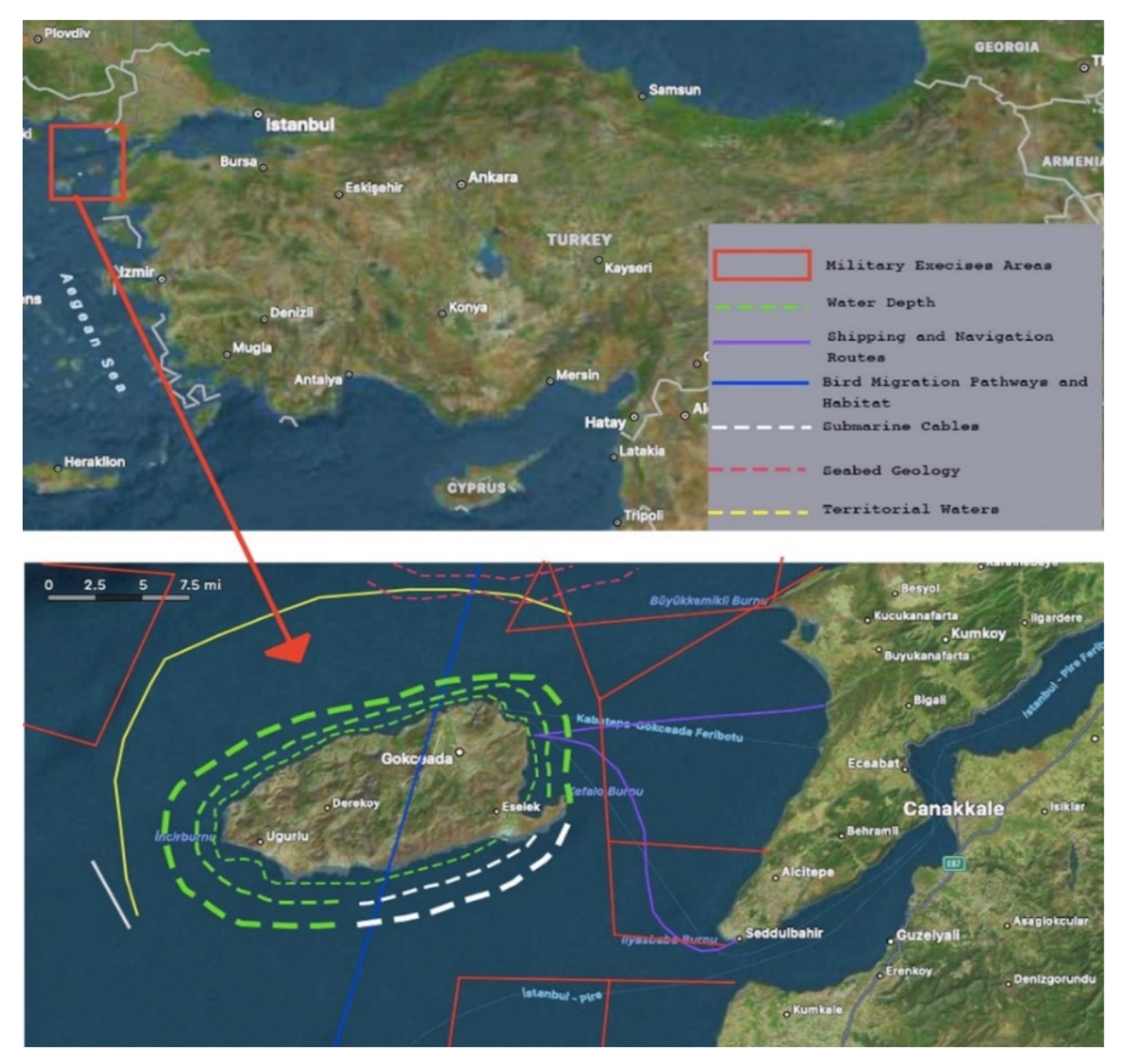
Gokceada Island is located in the Aegean Sea (
Figure 1). Gokceada, whose ancient name is Imbros (Imbros), is also Turkey’s largest island. It was formed on an area of 290 km
2 and is 11 miles (20 km) from Gallipoli Peninsula, 10 miles (19 km) from Limnos, and 12 miles (22 km) from Samothrace Island. Gokceada consists of 12% hilly, 11% plains, and 77% mountainous. The unusable land on the island is 30%. There are five ponds on the island, and it is the richest island on the Aegean in terms of water resources [
32].
Gokceada is open to the winds and generally, northeastern and southwestern winds are active. The island’s 2021 population is 10,377 and has seen an increase of 4% compared to 2020 and 10% compared to 2019 [
33]. The Uludag Electricity Distribution Company (UEDAS) is the only company responsible for electricity supply on this island due to the increasing use of new technologies and increasing population. Daily electricity demand depends on economic activities and the weather conditions.
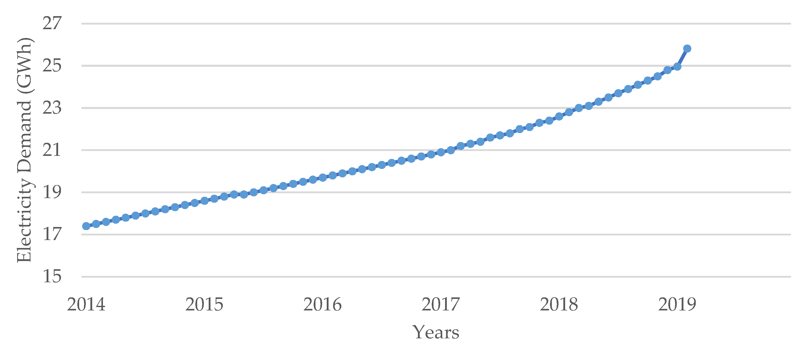
This study was conducted on Gokceada’s electrification system to assess which socio-economic variables have more effect, in terms of managing electricity demand growth. First, we proceeded to collect monthly electricity demand data for the period 2014 to 2019 from the Turkish Electricity Transmission Corporation and Uludag Electricity Distribution Company [
34,
35], to understand a better perspective of the historical trend. The electricity demand time series can be seen in
Figure 2, which shows a linear increase in the electricity demand.
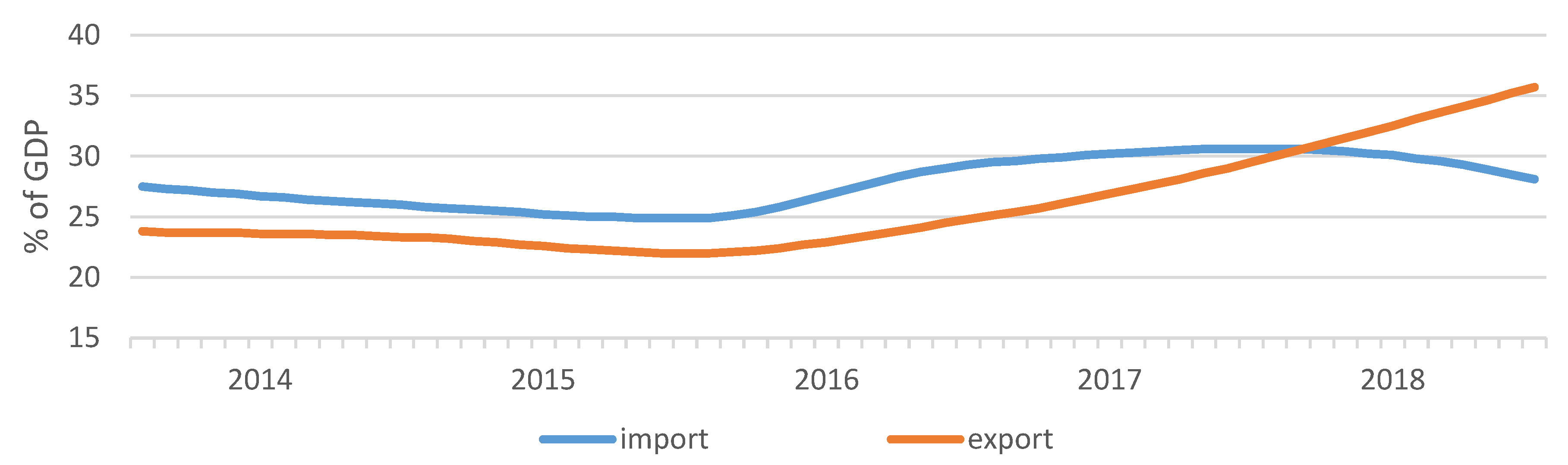
The next step of the data search consisted of identifying which variables had the most effect on forecasting island electricity demand. Five input variables were identified to design the model, which involves socio-economic indicators and energy consumption in gigawatt-hours (GWh). Population is taken from the Turkish Statistical Institute [
33]. Import and export values are taken from the World Bank Open Dataset (
Figure 3) [
36].
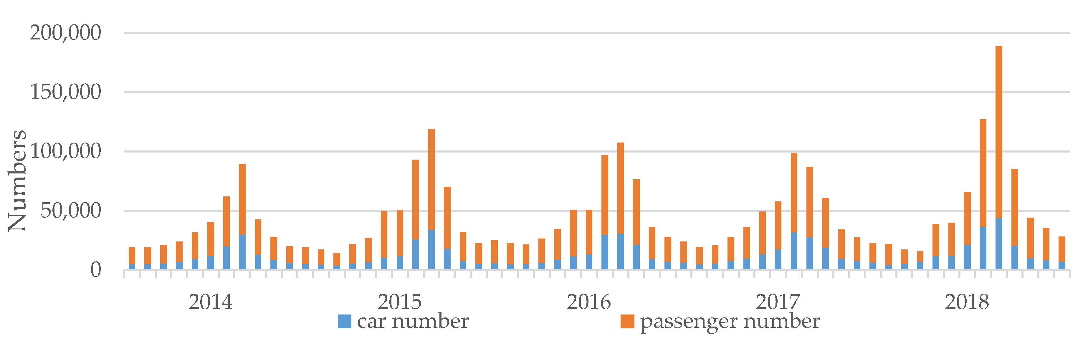
Gokceada Island monthly passenger, tourist, and car numbers were collected from GESTAS Maritime Transport Company (
Figure 4). The monthly economic services are also an important indicator that estimates the activity of 10 different economic sectors in Gokceada such as electricity, transportation, water supply, agriculture, etc.
Each variable was sketched to determine which ones showed a similar pattern to the electricity demand (
Figure 3 and
Figure 4). It was clear that import−export and car-passenger numbers exhibited a similar long-term pattern amongst themselves.
Data preprocessing was essential prior to creating and training the models. First, all the variables were merged and arranged into one excel file with a suitable format. The file was uploaded in MATLAB. Then, the entire data set was split into the training set (70%), test set (20%), and validate (10%), while preserving the temporal order of the data. Data from January 2014 to February 2017 were used as the training set, data from March 2017 to May 2018 were used as the test set, and data from June 2018 to December 2018. This process was applied to all the models.
3. Materials and Methods
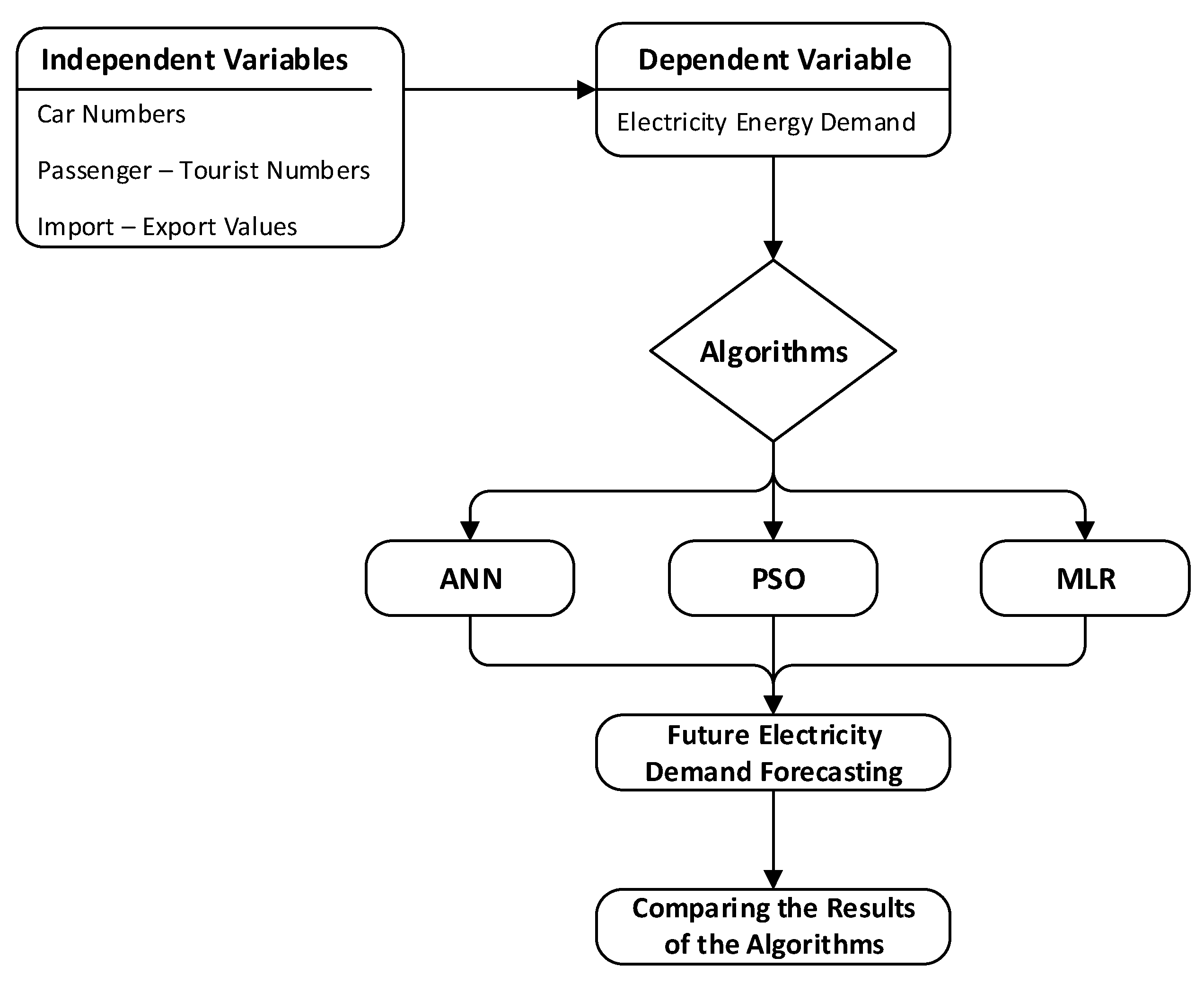
In this study, ANN, PSO (quadratic and linear), and MLR (quadratic and linear) forecasting methods were used to train, test, and validate historical energy consumption data, as can be seen in the methods flowchart in
Figure 5. Then, by using past demographical and economical input data, electricity demand was predicted up to 2040.
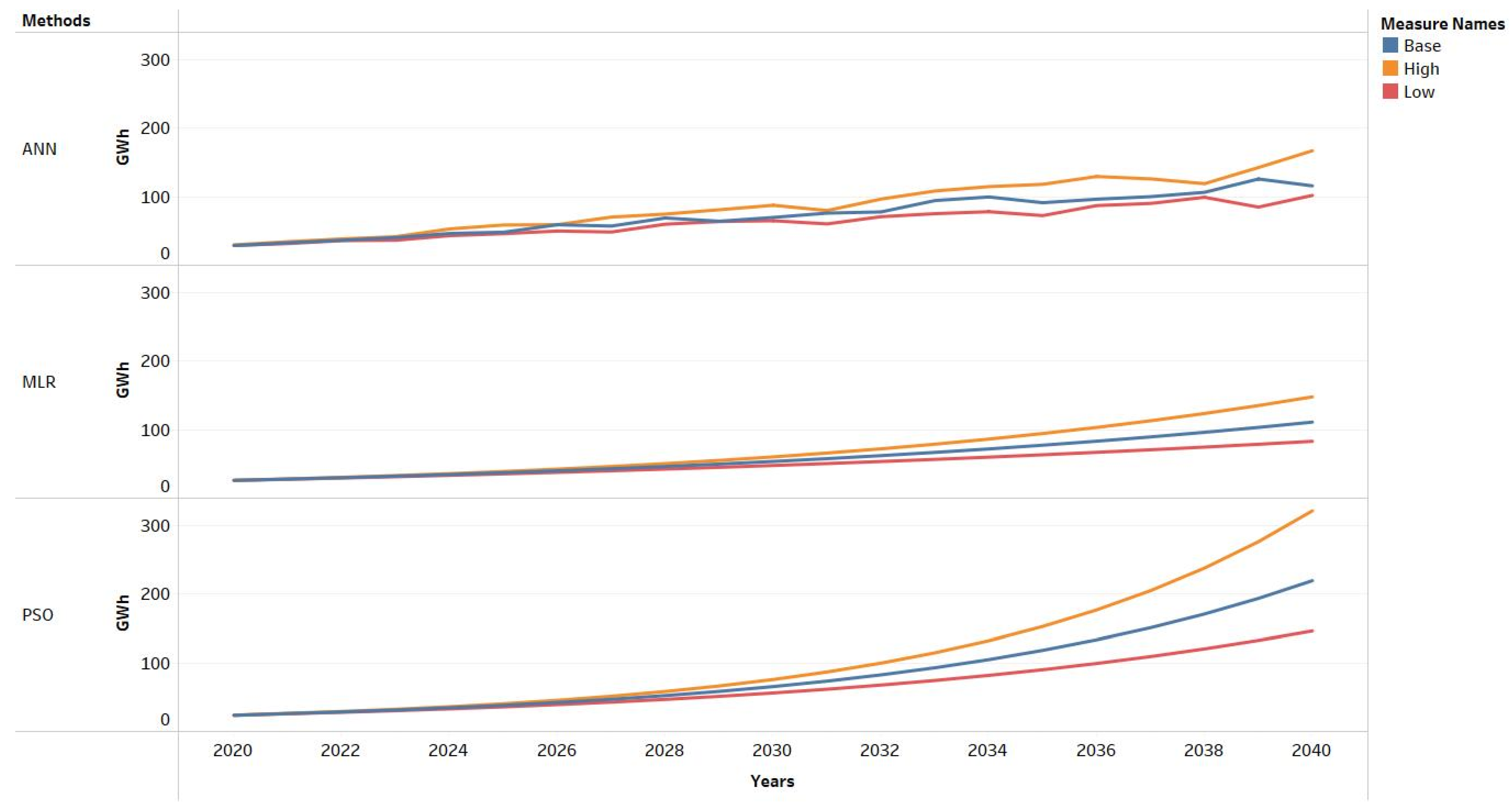
Each method includes three different scenarios: low, base, and high. Scenarios are designed by considering the proportional differences of the historical values of the input data used in the methods. Therefore, different input values and scenario ratios are used for Gokceada.
Table 2 shows scenarios and assumption of this island to forecast future electricity demand data.
3.1. Artificial Neural Networks (ANNs)
ANNs are an information processing technique inspired by the human brain information processing technique. With ANN, the biological neural system is imitated. ANN is composed of layers where artificial neurons are placed, and computational processes are performed [
37]. Within ANN, to process information, layers are linked to one another between input and output. The human brain and ANN are similar to each other in two aspects. The first aspect is the generation of knowledge within the network, which is performed via a learning process. The second aspect is the storage of the knowledge which is stored in the interneuron weights that synaptic connections resemble like the human brain [
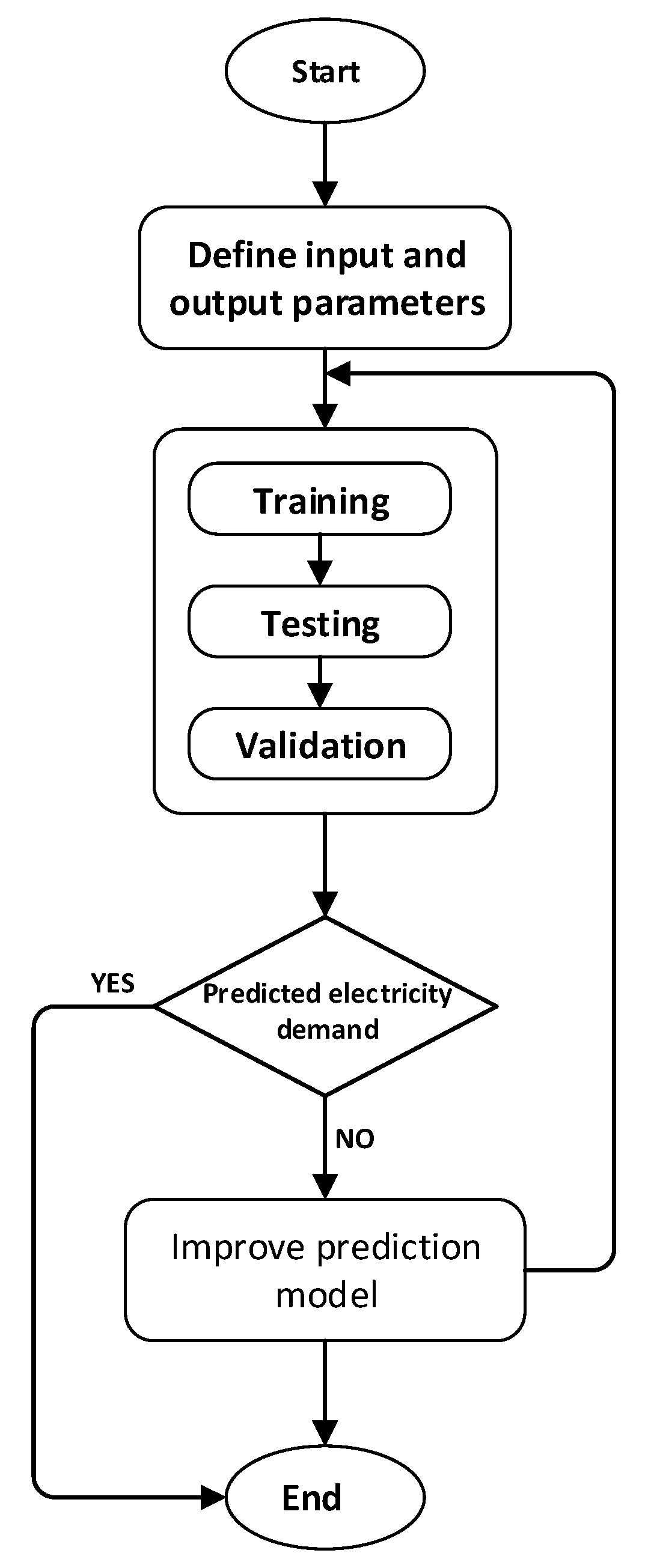
38]. The methodology for forecasting electricity demand with the use of ANN is schematically described in
Figure 6.
Within this study, a feed forward multilayer perceptron neural network was used to model the proposed forecasting electricity demand problem in Gokceada. Within the multilayer perceptron neural networks, the neurons and the layers are organized in a feed forward way. With this structure, the neurons’ input layer gathers the information from the system outside and the output layer calculates values based on the input data [
39].
In this study, to train the model, back propagation with gradient descent is used. The technique is called backpropagation and works as follows; first it compares the output value with the target, and then to reduce the error meaning of difference between output and target values, goes back to the input and changes network neuron weights. Within the back propagation, the Levenberg-Marquardt algorithm is used as the gradient-based algorithm.
Within the back propagation technique, if the weight combination that minimizes the error function is obtained, then the result is found. To guarantee the error function differentiability and continuity, transfer function between neurons is used [
40]. Within the feed forward multilayer networks, Sigmoid logistic transfer functions are often used within the hidden layer neurons while linear transfer function is used within the output neurons layer.
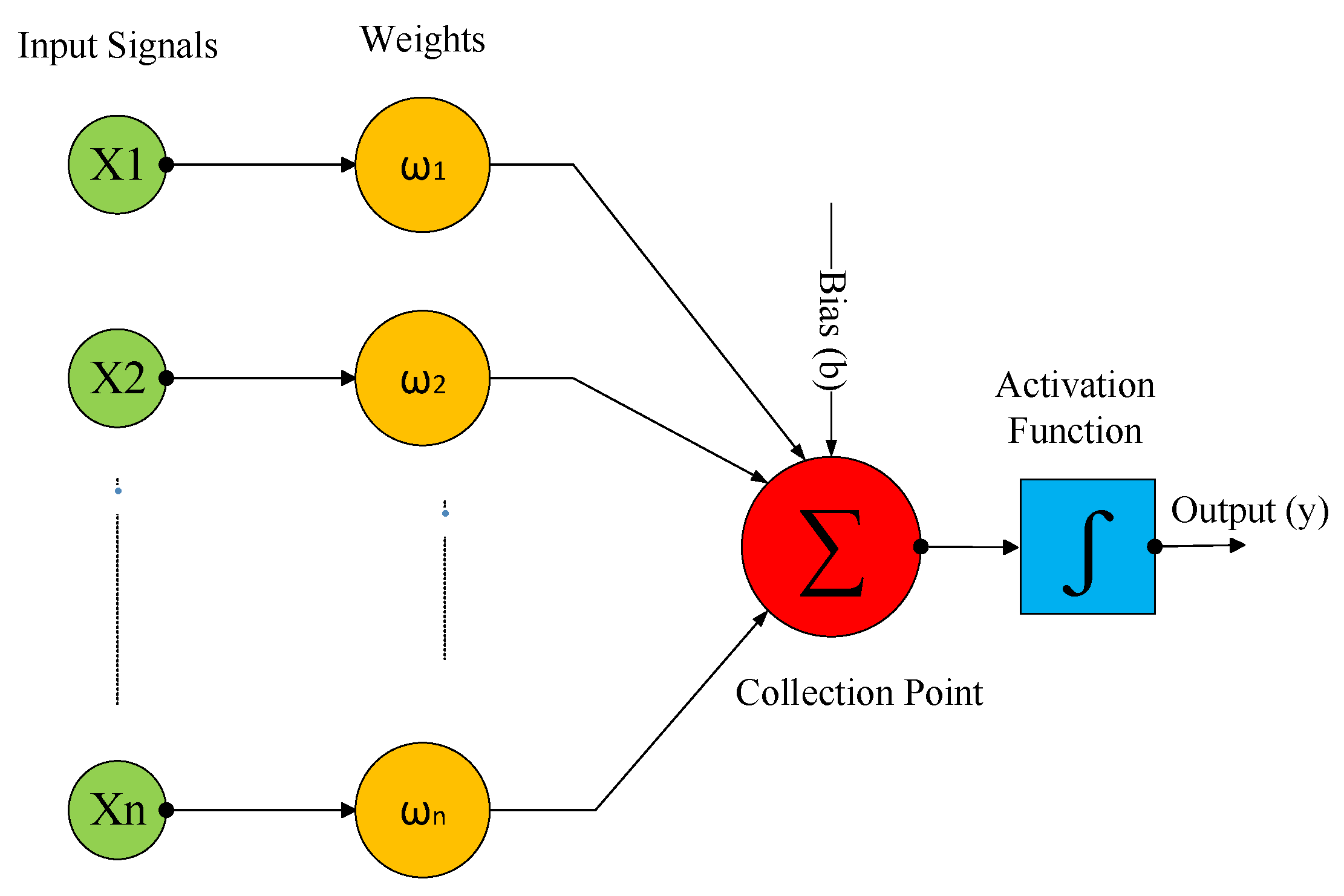
Every neuron is connected to a neuron within the next layer with weights. Every neuron, other than the neuron within the input layer, gets the weighted sum of all the neuron values in the previous layer, and the output value is calculated via putting the weighted sum in the transfer function [
41]. To represent this mathematically below, the neuron output is calculated using the Equations (1) and (2):
where
f represents the transfer function,
i is the input number,
y resembles the output value,
a is the inputs weighted sum,
w is the weight, and
j is the neuron number.
The sigmoid transfer function is defined with Equation (3):
Within the ANN that is represented within the below figure, ANN consists of three components which are input, hidden layer, and output (
Figure 7). Weights are assigned for all links between the layers. In
Figure 7, inputs are received by the input layer, then multiplied by the link weights between the hidden layer and the input layer and after that transmitted to the hidden layer. The inputs that are received by the hidden layer are transmitted to the output layer after multiplying them with the link weights which are between the hidden layer and the output layer. The activation function processes them and produces a suitable output. The link weight values are specified during the learning process [
42].
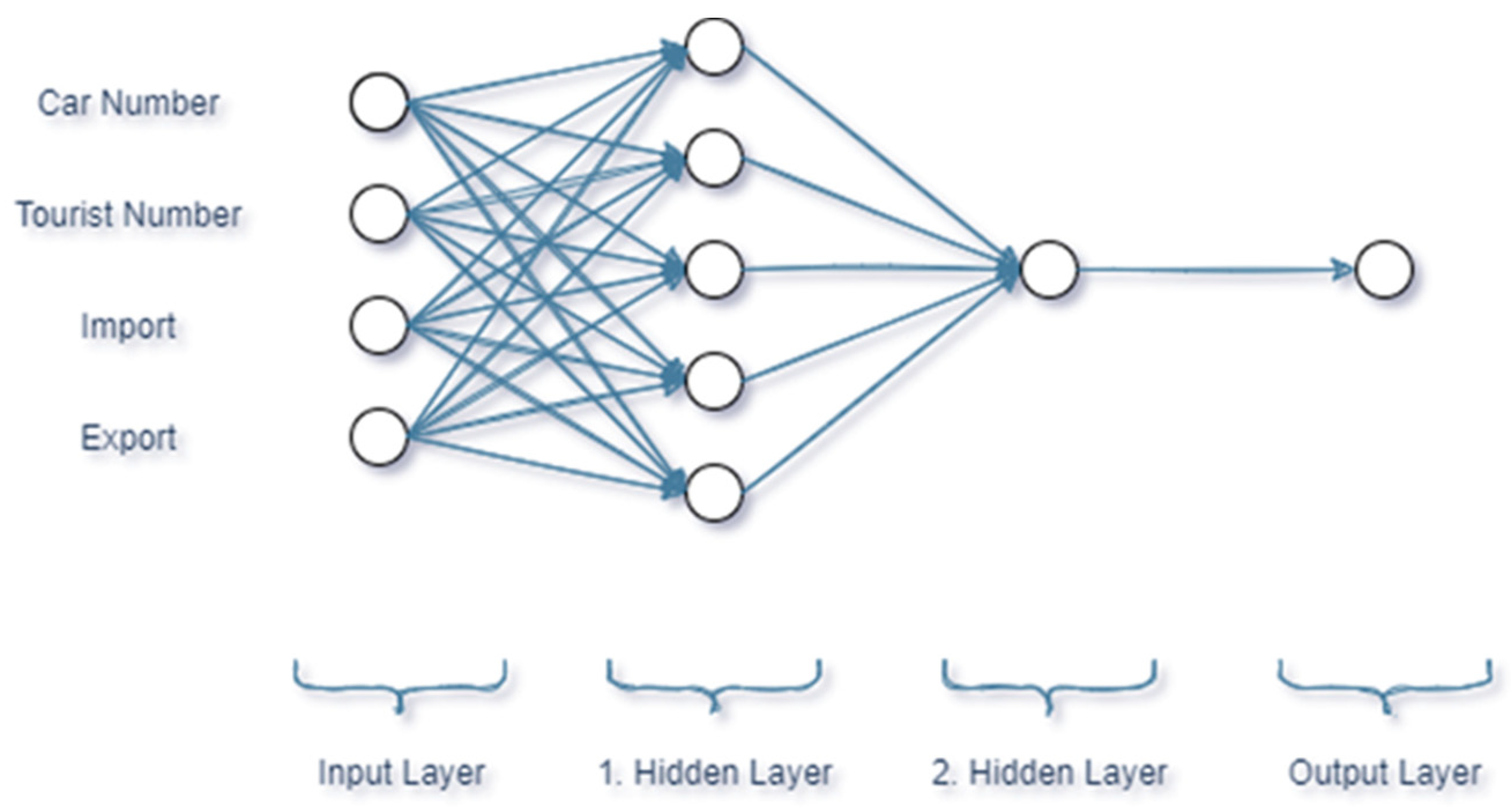
MATLAB Neural Network Toolbox was used for design, train, and simulate. Using this program, a neural network model was created, trained, and tested using available test data composed of 60 different data samples gathered from official sites. The data used in the neural network model are composed for input parameters that include car number, passenger, import, export and of format output parameter that include electricity consumption energy as shown in
Figure 8.
The components of an ANN model are as follows: inputs, transfer function, layers, training algorithm and number of neurons. All those components are variable, so could be changed, but any changes would result in the creation of a new ANN model which would also yield completely different results. In this study, the ANN method used the Levenberg−Marquardt algorithm as the training algorithm.
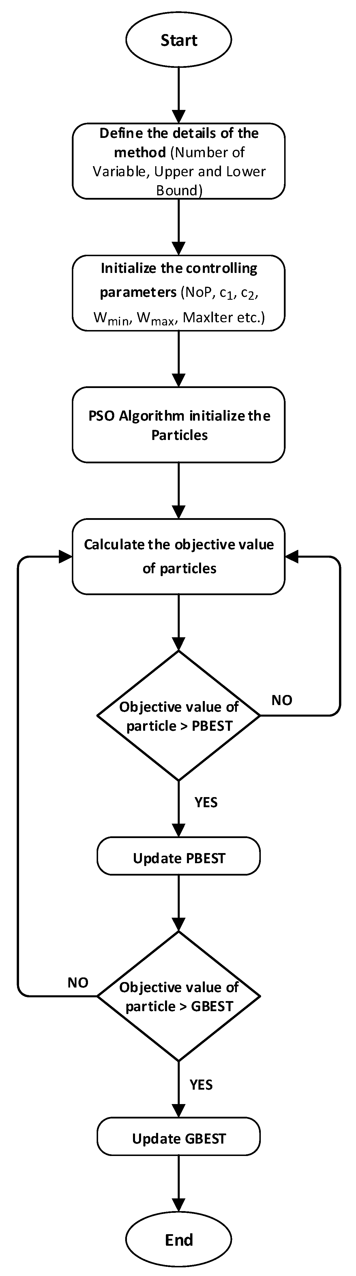
3.2. Particle Swarm Optimization (PSO)
The PSO algorithm was written by Kennedy and Eberhart in 1995. PSO is a swarm-based stochastic and intelligent algorithm that successfully solves optimization problems in all kinds of fields [
43,
44].
In this method, each possible solution known as a swarm represents population particles. In this approach, the particle position changes continuously in a multidirectional search region until it reaches the optimal response and/or computational constraints. The speed of approaching the solution is a situation that develops randomly, and most of the time individuals in the herd are in a better position in their new movements than in the previous position. This process ends when the goal is reached. Some studies given in the literature have shown the effectiveness and usefulness of this approach for optimization purposes [
45].
In the PSO algorithm, the velocity and position definition for each particle are the most important parameters. The following stochastic and deterministic renewal rules show how a particle’s velocity and position are refreshed. To determine the next position of the particle, the velocity and the new position vector are obtained by equations 4 and 5, respectively, using the information about the positions of the particle up to that point.
The velocities of all particles are represented by the velocity vector shown in Equation (4).
The velocity vector has three components. The first is velocity multiplied by w. Here, w is the inertia coefficient, a term required to maintain the current velocity. It also tries to maintain the current direction of movement. The second is the cognitive component. They are also called individual components in the literature. This can be said to be the distance of each particle’s location from each particle’s best value (PBEST). The last component is called the social component. This component specifies how far each particle is from the best value (GBEST) the entire swarm team has ever found. The coefficients r1 and r2 in the formula are the coefficients used to make the algorithm stochastic, ranging from zero to one. At the same time, the coefficients c1 and c2 are used to weight the acceleration of stochastic terms. Upper and lower bound values are given randomly in the first step. The number of the particle value is 30, C1 and C2 values are 2 for each, maximum iteration (MaxIter) is 100, inertia Wmax is 0.9, and Wmin is 0.2.
The positions of each particle are represented by the position vector shown in Equation (5).
To find the next position
of each particle, the velocity value
in the next iteration is added to its current position (
). Position, velocity, PBEST, and GBEST values are constantly updated in each iteration. The subscript
i in the formulas represents the particles number and the superscript
t represents the iterations number. The velocities and positions of the particles shown in Equations (4) and (5) are constantly updated until the optimal solution is reached [
46].
In this study, Gokceada’s future electricity energy demand has been estimated using the PSO algorithm. As indicated in the flowchart shown in
Figure 9 for the PSO algorithm, first the details of the problem were determined.
3.3. Multiple Linear Regression (MLR) Modeling
The method that reveals the cause-effect relationship between the dependent and independent variables as a mathematical model is called the MLR model. An MLR model clearly defines the relationship between independent and dependent variables.
Figure 10 shows the MLR flowchart.
MLR methods are used in estimating electricity demand, where the dependent variable
y is a function of more than one independent variable
(x1, x2, …, xk) [
47]. The relationship is given by:
From Equation (6),
y shows the electricity demand, and
x1 and
x2 are the exogenous variables, whereas
a0,
a1, and
a2 are unknown regression coefficients. The unknown coefficients
a0,
a1, and
a2 can be solved through the MLR method by decreasing the sum of the predicted error squares.
a0,
a1, and
a2 show the effect of each independent variable on the dependent variable. Equation (7) can now be simplified to
In Equation (7),
a,
b, and
c are defined as regression parameters that relate the mean value of
y to
x1 and
x2, where
c represents any exogenous factor. The above equations can be denoted in matrix notation
where terms
y,
x,
β, and
Ꜫ are described through Equations (9)–(12).
where
x is the vector component demonstrating each independent parameter,
y is the scalar response, subscript
n demonstrates the number of historical observations, subscript
k indicates the number of independent variables,
β0 to
βk are scalar regression coefficients, and
ε1 to
εk are the model scalar noise terms (biases). Multiple linear regression techniques are applied to specify
β0 to
βk unknown coefficients.
In this study, the least squares-fit method is used to forecast the regression coefficients in the MLR model. Generating a fit using a linear model requires minimizing the sum of the residual’s squares. Generally, the residuals visual plot is used to have a good insight into the goodness of fit. The goodness of fit is also calculated by the Adjusted Coefficient of Determination
and Coefficient of Determination
(R2), which shows how closely achieved values match the model dependent variable. When the least squares method (i.e., F-test, RMSE, R-squared) to achieve zero error is applied to defined matrix notations, it will be:
By solving Equation (13),
a,
b, and
c parameters are calculated, where
y is the electricity demand,
n is the number of years being forecasts, and
x1i and
x2i are historical independent variables (
xni, depending on the independent variables number). The result of the electricity demand estimates can be obtained by substituting the regression parameters in Equation (7) [
48].
3.4. Error Metrics
In this study, some commonly used statistical criteria were used to interpret the prediction success of the ANN-PSO-MLR model.
Error metrics include mean square error (MSE), Pearson’s correlation coefficient (R), root mean square error (RMSE), mean absolute percentage error (MAPE), and mean absolute error (MAE). MAE and RMSE evaluate the forecasted value discrepancy and the closeness to the true value, respectively, avoiding the positive and negative errors and mutual counteraction in the prediction. MSE represents the forecasted value divergence from the actual value while MAPE highlights the precision of the forecasting techniques. MAPE helps to investigate the forecasting methods’ performance when diverse data sets are used. It is desired and required to have low MAPE, RMSE, and MAE values. In addition, R states the correlation between the real and forecasted values [
49].
R2 indicates how much of the changes in the dependent variable is due to the changes in the independent variable and should take value between 1
> R2 > 0. The closer the
R2 value is to 1, the better the fit of the regression line is said to be. In other words, it is said that the changes in the dependent variable are caused so much by the changes in the independent variable. The formulas for the
R2, RMSE, MSE, and MAE are given in Equations (14)–(17) [
50,
51,
52,
53,
54,
55].
Note: represent the predicted value, actual value, sample size, mean predicted value, and mean actual value, respectively.
5. Discussion
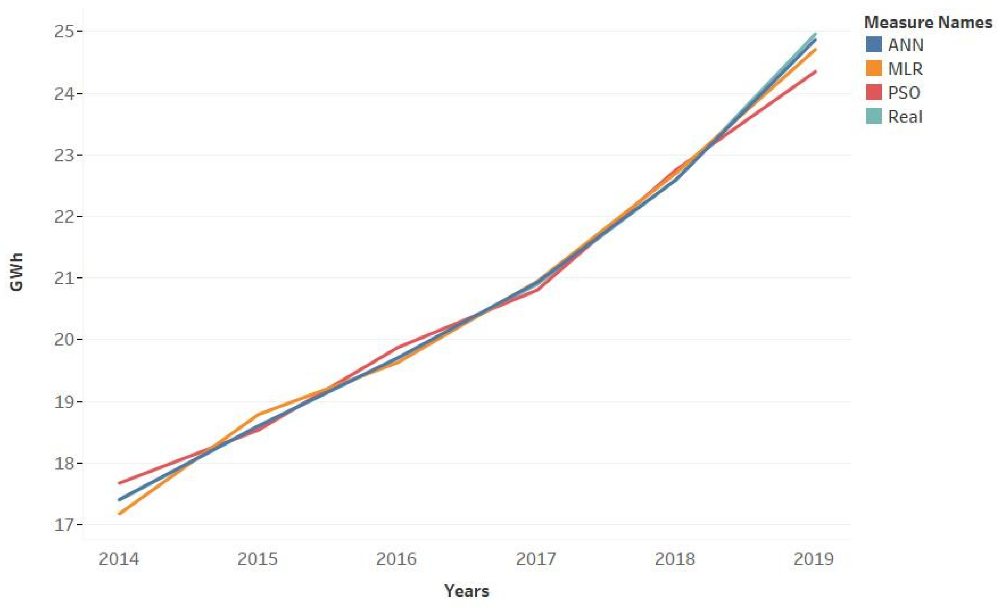
In this study, three different scenarios were implemented in ANN, PSO, and MLR models to forecast electricity demand for Gokceada Island. In Gokceada, import, export, car number, and passenger-tourist number were used as independent variables between 2014 and 2020. Data from 2014 to 2020 were used to generate linear and quadratic equations for the mainland. To validate the developed model, we used observed data between 2014 and 2020 and forecasted the future electricity demand until 2040 for the island. The model is used to estimate the Gokceada future electricity demand according to different scenarios.
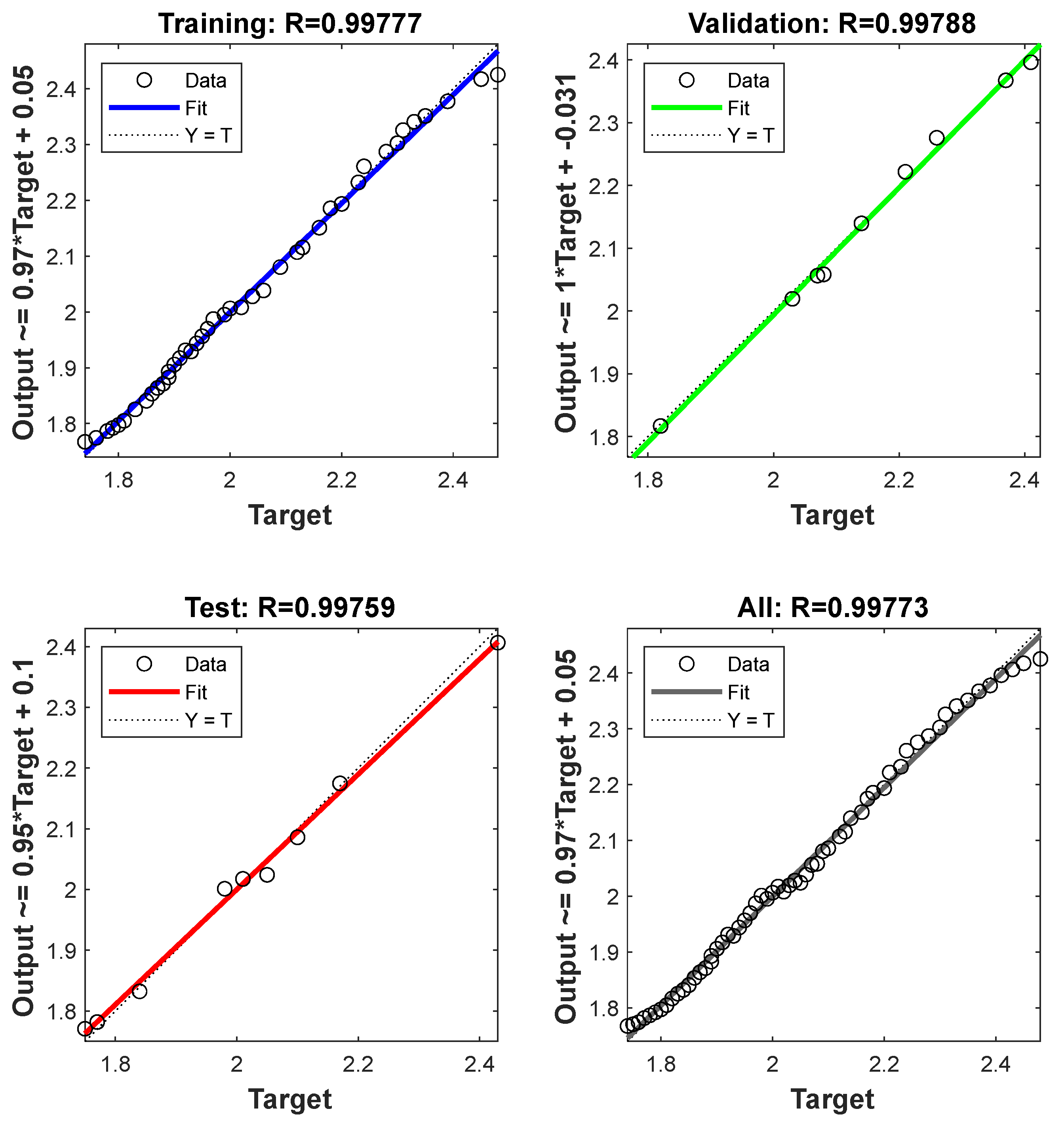
The R regression values for the training data set, validation data set, and test data set in the estimation of the electrical energy consumption of Gokceada Island from 2014 to 2019 by ANN are 0.9977, 0.9978 and 0.9975, respectively. The overall R regression value was calculated as 0.99773, which shows that ANN has very high reliability in estimating electrical energy consumption. The official results were very similar to those predicted by the ANN.
Import and export values are taken from the World Bank Open Dataset. Gokceada Island monthly passenger, tourist, and car numbers were collected from the GESTAS Maritime Transport Company. These variables are used in stepwise regression to determine which variables best estimate the dependent variable.
Statistical methods were used to test the significance of the correlation coefficient, and the results were compared. The correlation coefficient limits were obtained for the PSO, MLR, and ANN methods at the 95% confidence interval. Statistical method results reveal that ANN gives much better results at a 95% confidence interval and is a consistent method. The ANN technique’s flexibility makes it suitable for determining optimal solutions regarding the electricity demand forecasting future trends. Additionally, the obtained regression models’ high values show that ANN is an effective tool for the electricity demand forecast. This is required for the improvement of highly productive and applicable energy policy planning. The results illustrate that the proposed model can be used actively and effectively to predict long-term electricity demand. The results obtained can be a guide for future electricity network structures.
In the literature, many studies have been carried out to predict electricity demand by using PSO, MLR, and ANN. Additionally, the algorithm confidence intervals used for electricity demand forecasting were obtained by statistical methods, and the results were compared. RMSE, MSE, MAE, R2, correlation matrix independent and dependent variables between methods, and multi regression equations correlation are used to measure the proposed model performance. The error metrics gave a clear indication of the accuracy and precision of the estimation techniques.
A single hidden layer is usually used to design ANN architecture, but ANN architecture such as neurons and hidden layers are specified by trial and error in many articles. The hidden layer neuron numbers affect recognition process accuracy and the training speed. The neuron numbers and interlayer numbers of ANN and PSO can be modified in future studies to evaluate their electricity demand forecasting performance.
R2 demonstrates that the suggested regression model has a very good fit. Historical electricity T-stat demand is greater than 2, which means that it is statistically significant. Historical data and electricity demand p-value states that the three are remarkable regressors and a meaningful addition to the model. It can be said that there is a strong linear relationship between export and electricity consumption (0.8974), and a low linear relationship between electricity consumption and car number (0.2228). In addition, car number and passenger investigate a strong linear relationship (0.9573).
Based on the analysis of the data, the following main conclusions were found in the study: it has been determined that the linear model of the first and second scenarios of the PSO have close estimated values. According to the second scenario in the quadratic form of the PSO, the energy demand has started to decrease since 2034. There may be various reasons for the decrease in energy demand after 2034. These may be reasons such as socio-economic problems, energy saving policies, renewal of power plants, and increasing their efficiency. First and second scenario prediction values are very close to each other in linear and quadratic forms of MLR. When the estimations of the scenarios are compared, it is concluded that the linear estimations of ANN and PSO are close to each other, and the quadratic estimation results of MLP and PSO are close to each other.
Future studies must obtain more data, increase the number of inputs, and analyze the effects on future electricity demand forecasting results. It is planned to carry out a study that includes hybrid and machine learning methods. Further, different optimization techniques can be designed to evaluate the learning models’ forecasting accuracy.


