A Log-Logistic Predictor for Power Generation in Photovoltaic Systems

Abstract

Photovoltaic (PV) systems are dependent on solar irradiation and environmental temperature to achieve their best performance. One of the challenges in the photovoltaic industry is performing maintenance as soon as a system is not working at its full generation capacity. The lack of a proper maintenance schedule affects power generation performance and can also decrease the lifetime of photovoltaic modules. Regarding the impact of environmental variables on the performance of PV systems, research has shown that soiling is the third most common reason for power loss in photovoltaic power plants, after solar irradiance and environmental temperature. This paper proposes a new statistical predictor for forecasting PV power generation by measuring environmental variables and the estimated mass particles (soiling) on the PV system. Our proposal was based on the fit of a nonlinear mixed-effects model, according to a log-logistic function. Two advantages of this approach are that it assumes a nonlinear relationship between the generated power and the environmental conditions (solar irradiance and the presence of suspended particulates) and that random errors may be correlated since the power generation measurements are recorded longitudinally. We evaluated the model using a dataset comprising environmental variables and power samples that were collected from October 2019 to April 2020 in a PV power plant in mid-west Brazil. The fitted model presented a maximum mean squared error (MSE) of $0.0032$ and a linear coefficient correlation between the predicted and observed values of $0.9997$. The estimated average daily loss due to soiling was $1.4\%$.

1. Introduction

1.1. Impact of Soiling on Power Generation in Photovoltaic Systems

Photovoltaic (PV) systems have a high penetration capacity with a low environmental impact [1]. Some countries are more suitable as sites for PV plants due to their high solar irradiation. Brazil, for example, has vast solar energy potential, mainly in the northeast region, which offers the highest average solar radiation and the lowest annual variability [2]. International agencies have predicted that the use of PV energy for worldwide power generation will increase from 2% in 2018 to 25% in 2050 [3].

One of the challenges in the photovoltaic industry is performing maintenance as soon as a system is not working at its full generation capacity [4]. The lack of a proper maintenance schedule affects power generation performance and can also decrease the lifetime of photovoltaic modules.

One source of power generation loss is soiling on PV modules. Soiling may attenuate solar irradiation on the PV cells, thus reducing their photovoltaic effects and energy generation capabilities. The uniform dispersion of soiling affects spectral transmittance, which is a characteristic of photovoltaic technology that is used to construct the modules [5]. Suspended particles in the air are one of the primary sources of soiling. The average annual losses in the performance of solar plants due to soiling range from $3\%$ to $6\%$, while monthly evaluations indicate power losses from $14\%$ to $20\%$ [6,7]. Correctly understanding soiling deposition patterns is crucial to solving this problem.

Soiling particles in the air change according to the environment, leading to different impacts depending on the location of the photovoltaic system [8]. Regarding the endemic features of soiling, the monitoring of environmental parameters and suspended particles in the air should be local (within the PV power plant site) and continuous. Understanding the economic implications of soiling on photovoltaic systems is essential to increase energy production, optimize cleaning routines and minimize the associated costs [9]. The concern around the impacts of soiling on PV energy generation is primarily due to the increase in the number of large-scale PV power plants in isolated regions that are exposed to high soiling levels. The online monitoring of PV systems can benefit decision-making regarding the maintenance and cleaning of PV modules to reduce the impacts of soiling on power generation [10].

1.2. Related Work

Many studies have proposed power loss estimates from soiling on PV power plants [11]. The proposed techniques range from applying images (from cameras and satellites) and computer vision algorithms to adopting environmental sensors to identify and estimate the impacts of soiling on power generation.

Mehta et al. [12] determined the impacts of soiling by designing models that were based on convolutional neural networks (CNNs), the RGB images of solar panels and environmental variables. The authors presented the impacts of soiling on power loss and achieved an accuracy of up to 97.82%. Another soiling identification technique was based on finding “hot spots” on photovoltaic modules [13,14]. This technique was carried out using radiometric sensors that showed a high degree of reliability compared to thermographic cameras and achieved an accuracy of 99.02% and a precision of 91.67%.

Pavan et al. [15] compared two techniques to determine the effects of soiling on large-scale photovoltaic plants. The experiment was carried out at two solar plants in different sites in Italy. The authors developed prediction models using a Bayesian neural network (BNN) and a polynomial regression model (PRM). PRMs have also been used in previous research on the same systems [16]. The power loss due to dust particle accumulation on the PV systems ranged from 1% to 5%.

The cleanliness index (CI) [17] has also been applied to evaluate performance loss that is caused by soiling. Those authors used an artificial neural network (ANN) and multilinear regression (MLR) to estimate the CI. As reported by the authors, the ANN model achieved better results than the MLR model (ANN: $R^2=0.54$; MLR: $R^2=0.17$). The authors also observed that wind speed and relative air humidity were the environmental variables that had greater effects on the amount of dust that was transported and accumulated on the PV modules.

Hammad et al. [18] studied the impacts of soiling on PV power plants in the Middle East and North Africa (MENA) region. The authors highlighted the usage of MLR and ANN models to estimate the impacts of soiling on power loss and the optimal momentum to clean the modules in the PV systems. The models considered dust exposure time and environment temperature as the independent variables and the PV system conversion efficiency as the dependent variable. Once all of the losses due to inverters, array mismatch, operating environment temperature and dust accumulation were taken into account, the authors could eliminate the dust effect. So, the difference between the conversion efficiency before and after that elimination corresponded to the soiling impact [19].

1.3. Statistical Methodology for Soiling Estimation

The power generation predictor that is proposed in this work was based on the fit of a nonlinear mixed-effects (NLME) model, according to a log-logistic function. The primary motivation for considering a log-logistic model was that log growth models can adequately model the accumulated measurements of generated power over the course of a day. Random effects were introduced to model the correlations among the measurements of generated power since they were recorded longitudinally. In addition, we considered irradiance and the accumulated mass (soiling) on the photovoltaic modules as the explanatory (independent) variables.

In order to estimate the model parameters, we adopted the maximum likelihood method. The estimates were obtained numerically using the algorithm that was proposed by Lindstrom and Bates [20]. We then illustrated the performance of the proposed model using a dataset comprising power generation and environmental (environment temperature, irradiance and the mass of the particles on the modules) samples that were collected from a photovoltaic plant located at the Federal University of Mato Grosso do Sul (lat.: −20.510867; long.: −54.619882). The model validation and evaluation were performed by comparing the mean squared errors (MSEs) of the predicted (from the NLME model) and the observed (from the PV power plant) generated power values.

2. Materials and Methods

The experimental data were collected from a PV power plant on the campus of the Federal University of Mato Grosso do Sul (lat.: −20.510867; long.: −54.619882). The plant comprises 38 PV modules (275 Wp) of polycrystalline silicon (poly-Si) (model CS6K-275P), which are organized into two strings of 19 modules and form an array with a maximum power of 10.45 kWp. The PV power plant has an 8.2-kW Fronius inverter (model Primo 8.2-1) with two MPPT inputs and internet connectivity.

The environmental and soiling monitoring system that was available in the PV plant was based on an ESP32 electronic platform (NodeMCU ESP32). The sensors that were used to collect the environmental data were a pyranometer (Hukseflux SR05-DA2) for measuring radiation at the site of the photovoltaic system, a temperature sensor (DS18B20) and a sensor for detecting suspended atmospheric particulates (Sensirion SPS30), all of which collected data every 1 min. The electronic platform collected, gathered and controlled the environmental and soiling measurements from the sensors and the generated power data from the inverter. All of the data were then sent to an AWS cloud server (there was a wireless internet connection available at the PV plant site).

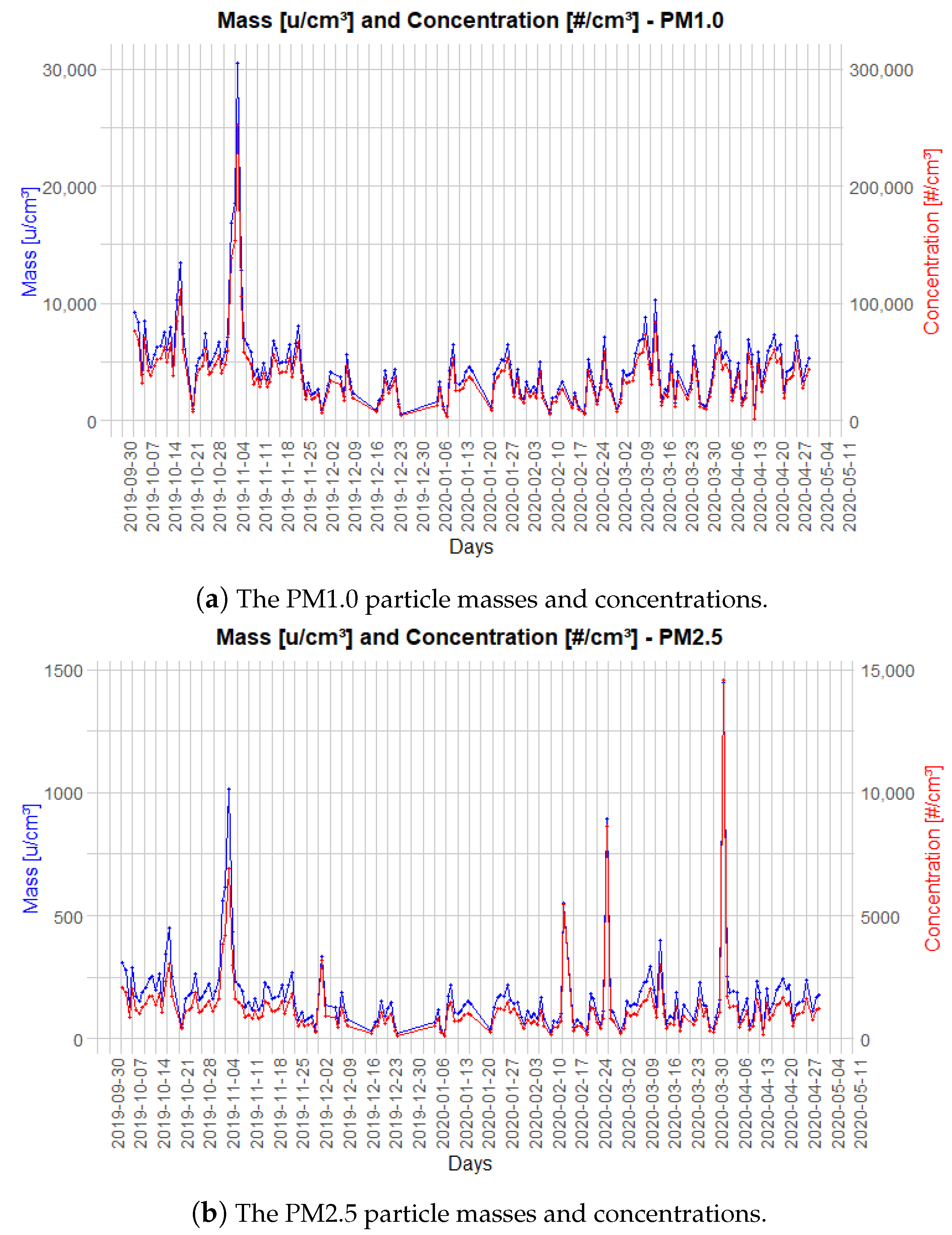
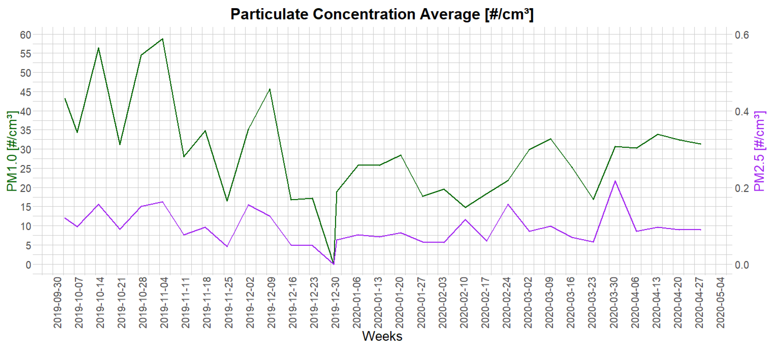
2.1. Estimation of Accumulated Particle Mass

According to El-Shobokshy and Hussein [21], Hupa et al. [22] and Javed et al. [17], the estimation of the particle mass on PV modules relies on several parameters, such as chemical composition, the properties of the module surface, wind speed and air particle suspension. Coello and Boyle [23] proposed to estimate the particle mass deposition on PV modules using the following equation:

$$M=(v_{10-2.5}{C}_{10-2.5}+v_{2.5}{C}_{2.5})tcos\left(\theta \right)$$

(1)

where:

• M is the accumulated mass in the time interval (g/${\mathrm{m}}^2$);
• t is the time interval in seconds;
• v is the particulate deposition speed (g/m);
• C is the particulate concentration in the environment (g/${\mathrm{m}}^3$);
• $\theta$ is the PV module angle;
• _10−2.5 is the index of the particles from 10 μm to 2.5 μm;
• _2.5 is the index of particles less than 2.5 μm.

At the PV plant location in this work, the particle sensor did not detect particles above 2.5 μm, so Equation (1) was adjusted for particulates below 2.5 μm. Other adjustments to the original model were also necessary, such as the sensor height, module tilt and constant values. Figure 1 depicts the typical behavior of the particles that was captured over the course of a day by the Sensirion SPS30 sensor at the PV power plant site. PM1.0 and PM2.5 represent the particulate material identified in the environment with diameters up to 1.0 and 2.5 μm, respectively.

Figure 2 presents the PM1.0 and PM2.5 particle masses and concentrations over the course of seven months, from October 2019 to April 2020. Figure 3 presents the weekly particle concentration averages. From 23 December to 3 January, the particle sensor was not functional, so there were no data collected during this short period.

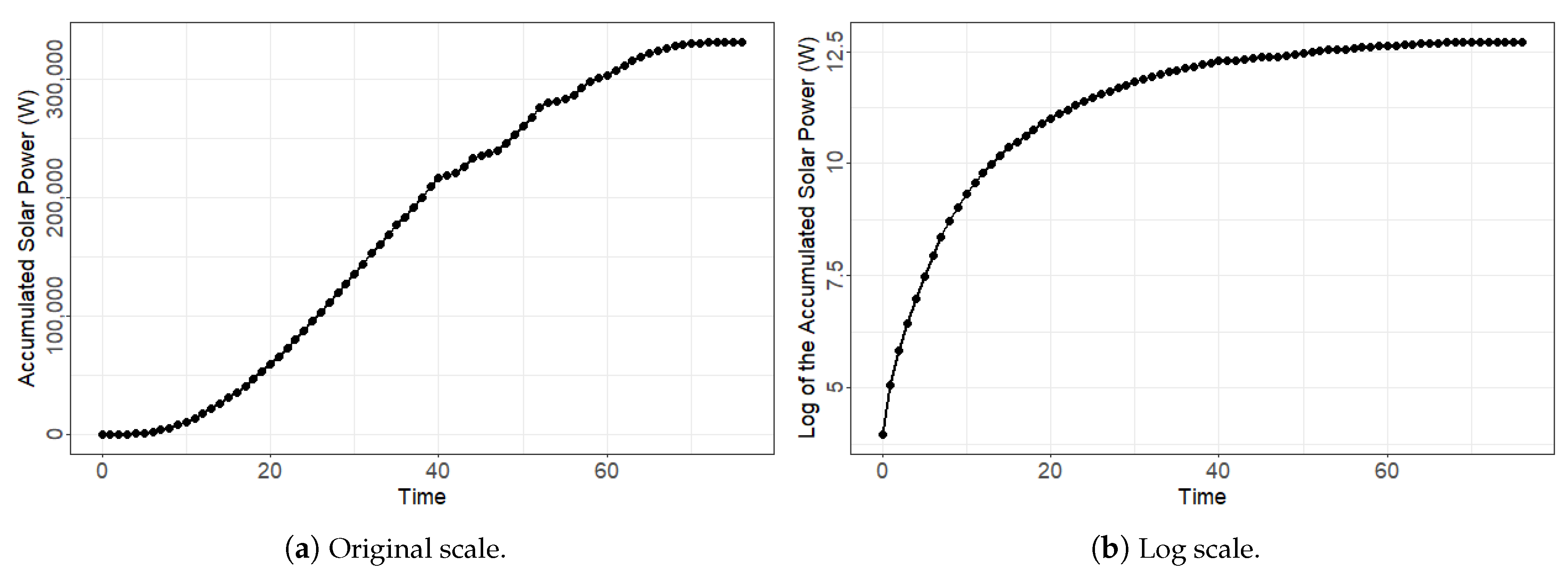
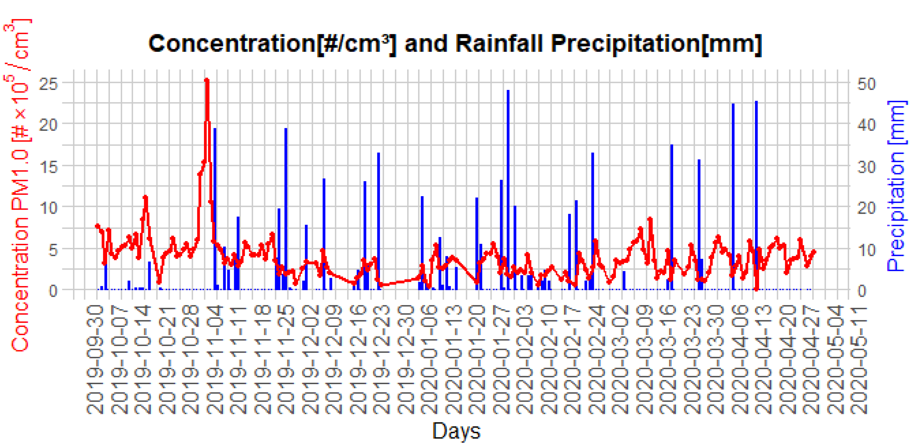
2.2. Dataset and Statistical Modeling

We let $\mathbb{D}$ be the dataset comprising the measurements of the PV-generated power and the environmental variables (temperature, irradiance and the accumulated mass of particles) from a period of $d=105$ days.

In order to build this dataset, we assumed the following procedure. For each day, the environmental and generated power data were registered every $r=10$ minutes throughout the period between the first and last samples of solar irradiance (the start and the end of each day). On the j-th day, there were $n_j$ measurements of PV-generated power, temperature, irradiance and particle mass for $n_j\in {\mathbb{Z}}^{+}$ and $j=1,\dots ,d$, where ${\mathbb{Z}}^{+}$ represents a set of positive integers.

Figure 4 shows the generated power, irradiance, temperature and accumulated mass measurements that were recorded on days 1 and 2. The generated power, temperature and irradiance are represented in the log scale to better visualize the plot. The values for the accumulated mass are in the original scale. Regarding day 1, the first measurement was recorded at 06:12 am and 74 measurements (x axis) of each variable were taken in total. On day 2, the first measurement was recorded at 06:14 am and 72 measurements of each variable were taken. The behavior of the PV-generated power and irradiance was pretty similar. The values of the estimated soiling (from the accumulated mass of particles) were near zero on the two first days because the experiment began just after a clean-up procedure was carried out on the PV modules.

We split dataset $\mathbb{D}$, which had data samples from 105 days, into two sub-datasets: ${\mathbb{D}}_0$ and ${\mathbb{D}}_1$. Dataset ${\mathbb{D}}_0$ was the training set, which was composed of measurements from the first 21 days and was used to fit the prediction model. Dataset ${\mathbb{D}}_1$ was the testing set, which had measurements from the last 84 days and was applied to verify the performance of the fitted prediction model.

Table 1. The summary of the measurements.

Variable	Measurements
	Min.	1st Q.	Median	Average	S. Deviation	3rd Q.	Max.
Power	2.77	997.19	3616.73	3858.56	2882.368	6528.59	8475.12
Irradiance	0.10	118.60	420.40	470.50	362.37	799.30	1197.20
Temperature	19.15	27.63	31.36	30.80	4.67649	34.71	39.34
Accumulated Mass	0.1387	0.1971	0.2599	0.2768	0.08948	0.3720	0.3920

shows a summary of the main descriptive statistics of the training set ${\mathbb{D}}_0$. The generated photovoltaic power ranged from 2.77 W to 8475.12 W, with an average of 3858.56 W. The irradiance values ranged from 0.10 W/${\mathrm{m}}^2$ to 1197.20 ${\mathrm{W}\mathrm{/}\mathrm{m}}^2$, with an average of 470.50 ${\mathrm{W}\mathrm{/}\mathrm{m}}^2$. The environment temperature ranged from 19.15 °C to 39.34 °C, with an average of 30.80 °C. The maximum accumulated mass of particles during the period was 0.3920 μg/${\mathrm{m}}^3$.

The statistical model assumed that no linear relationship existed among the explanatory variables. We applied Pearson’s correlation for each pair of variables from ${\mathbb{D}}_0$ (

Table 2. The Pearson’s correlations.

Variable	Variable
	Irradiance	Temperature	Accumulated Mass
Irradiance	1	0.6754	−0.2226
Temperature	0.6754	1	−0.5231
Accumulated Mass	−0.2226	−0.5231	1

). On the one hand, the irradiance and temperature had a strong positive linear relationship. On the other hand, irradiance had a weak correlation to the accumulated mass and the temperature and accumulated mass had a moderate correlation. Since there was a linear correlation between irradiance and temperature, temperature was disregarded for the model fit.

We let $W_{tj}$ be the recorded power that was generated at the t-th instant in time on the j-th day for $t=1,\dots ,n_j$ and $j=1,\dots ,d$. Analogously, we let $I_{tj}$ be the irradiance that was recorded at the t-th instant in time on the j-th day. The accumulated mass of particulates $M_{tj}$ (accumulated mass) on the PV system was calculated according to Equation (1).

As illustrated in Figure 4, the $W_{tj}$ values had a high variability and demonstrated an unstable nonlinear behavior, making a linear modeling procedure somewhat complicated. We developed a modeling procedure that considered the power that was generated once those values presented a more stable behavior. Figure 5 shows the solar power that was generated over the course of a day, in both the original and log scales.

For simplicity, we left the index j out and used $W_t$ to denote the solar power that was generated at the t-th instant in time on the j-th day. Similarly, we used $I_t$ and $M_t$ to represent the irradiance and the accumulated mass of particulates that were recorded at the t-th moment on the j-th day.

2.3. Nonlinear Mixed-Effects Model

We let ${\mathbb{X}}_t$ be the generated power at the t-th instant in time on a given day:

$${\mathbb{X}}_1=W_1\mathrm{and}{\mathbb{X}}_t=\sum _{i=1}^t{W}_i$$

for $t=2,\dots ,n_j$. Similarly, we let ${\mathbb{I}}_t$ be the recorded irradiance at the t-th instant in time on that day.

We assumed that the ${\mathbb{X}}_t$ values were generated according to the following model:

$${\mathbb{X}}_t=h\left(t\right|{\theta }^{\prime })·{\nu }_t,$$

(2)

where $h\left(t\right|{\theta }^{\prime })$ is a nonlinear growth model, ${\theta }^{\prime }$ represents the parameters of the model and ${\nu }_t$ is a random error. Since ${\mathbb{X}}_t$ was a positive value, then we assumed that the random error ${\nu }_t$ came from a log-normal distribution with the mean μ and variance ${\sigma }^2$ of ${\nu }_t\sim \mathcal{LN}(\mathrm{\mu },{\sigma }^2)$ for $t=1,\dots ,n_j$.

We set $h\left(t\right|{\theta }^{\prime })$ as the logistic growth function [24]:

Comment 1.

$${\mathbb{Y}}_t=log\left({\mathbb{X}}_t\right)=f\left(t\right|{\theta }_0)+{\epsilon }_t$$

(3)

$$h\left(t\right|{\theta }^{\prime })=\frac{{\alpha }^{\prime }}{1+exp\{{\beta }_0-\gamma t\}},$$

(4)

where ${\theta }^{\prime }=({\alpha }^{\prime },{\beta }_0,\gamma )$ represents the model parameters for $t=1,\dots ,n_j$. This model had an S-shaped curve that was defined by two distinct phases. A positive slope characterized the first phase, which showed that the growth rate was increasing, and the second phase was characterized by a negative slope, which showed that the growth rate was decreasing. The point at which the slope of the curve changed (i.e., from positive to negative) was the inflection point. The coordinates of the inflection point were $\left(\frac{log\left({\beta }_0\right)}{\gamma },\frac{{\alpha }^{\prime }}{2}\right)$.

By applying a logarithmic transformation on both sides of Equation (2), the log-logistic model was given by:

$${\mathbb{Y}}_t=log\left({\mathbb{X}}_t\right)={\alpha }_0-log\left(1+exp\{{\beta }_0-\gamma t\}\right)+{\epsilon }_t,$$

(5)

where ${\alpha }_0=log\left({\alpha }^{\prime }\right)$ and ${\epsilon }_t=log\left({\nu }_t\right)$ for $t=1,\dots ,n_j$. Thus, we obtained ${\epsilon }_t\sim \mathcal{N}(\mathrm{\mu },{\sigma }^2)$ for $t=1,\dots ,n_j$. Hereinafter, we set $\mathrm{\mu }=0$. Likewise, we let ${\mathbb{Z}}_t=log\left({\mathbb{I}}_t\right)$ for $t=1,\dots ,n_j$.

To relate the response variable $\mathbb{Y}$ to the explanatory variables $\mathbb{Z}$ and M, we considered the following hierarchical model:

$$\begin{array}{ccc}\hfill {\mathbb{Y}}_t& =& ({\alpha }_0+A_t)-log(1+exp\{({\beta }_0+B_t)-\gamma t\})+{\epsilon }_t\hfill \\ \hfill A_t& =& {\alpha }_1{\mathbb{Z}}_t+{\alpha }_2{M}_t+a_t\hfill \\ \hfill B_t& =& {\beta }_1{\mathbb{Z}}_t+{\beta }_2{M}_t+b_t\hfill \end{array}$$

(6)

in which the vector of random effects $(a_t,b_t)$ is bivariate normally distributed with zero-mean and variance–covariance matrix:

$${\mathrm{\Sigma }}_e=\left[\begin{array}{cc}{\sigma }_a^2& {\sigma }_{ba}\\ {\sigma }_{ab}& {\sigma }_b^2\end{array}\right]$$

for $t=1,\dots ,n_j$.

Since the measurements were registered longitudinally, the errors could be heterogeneous and correlated. In order to model both structures of the dataset, we assumed that the vector of the random errors ${\epsilon }_j=({\epsilon }_1,\dots ,{\epsilon }_{n_j})$ from the j-th day, is generated from a $n_j$-variate normal distribution with vector-mean 0 and variance-covariance $R_j$ of dimension $n_j\times n_j$, for $j=1,\dots ,d$. This covariance matrix had to account for the heteroscedasticity and autocorrelation of the measurements that were registered on the j-th day. Following the proposal of Davidian and Giltinan [25] and Xu et al. [26], we considered:

$$R_j={\sigma }^2{\mathbb{G}}_j^{1/2}{\mathbb{H}}_j{\mathbb{G}}_j^{1/2},$$

(7)

where ${\mathbb{G}}_j$ and ${\mathbb{H}}_j$ are the $n_j\times n_j$ matrices that account for the error variance and autocorrelation of the measurements from the j-th day, respectively, for $j=1,\dots ,d$.

We modeled the variance as a power function by letting $varpower\left({\epsilon }_t\right)={\sigma }^2{t}^{2\delta }$ for a power of $\delta \in \mathbb{R}$. The matrix ${\mathbb{G}}_j$ was a diagonal matrix with the diagonal elements of $t^{2\delta }$ for $t=\{1,\dots ,n_j\}$ and $j=1,\dots ,d$. For the autocorrelation structure, we considered a first-order autoregressive model ($A{R}_1$). From this assumption, when ${\epsilon }_t$ and $\epsilon (t+s)$ were two random errors that were separated by s units of time, then $cor=({\epsilon }_t,{\epsilon }_{(t+s)})={\rho }^{\left|s\right|}$ for $t=1,\dots ,n_j$ and $j=1,\dots ,d$. Matrix ${\mathbb{H}}_j$ was given by:

$${\mathbb{H}}_j=\left[\begin{array}{ccccc}1& \rho & {\rho }^2& \dots & {\rho }^{n_d-1}\\ \rho & 1& {\rho }^2& \dots & {\rho }^{n_d-2}\\ ⋮& ⋮& ⋮& \dots & ⋮\\ {\rho }^{n_d-1}& {\rho }^{n_d-1}& {\rho }^{n_d-3}& \dots & 1\end{array}\right]$$

Using Equation (6), the proposed NLME model was given by:

$${\mathbb{Y}}_t={\alpha }_0+{\alpha }_1{\mathbb{Z}}_t+{\alpha }_2{M}_t-log(1+exp\{{\beta }_0+{\beta }_1{\mathbb{Z}}_t+{\beta }_2{M}_t-\gamma t+b_t\})+a_t+{\epsilon }_t$$

(8)

We let $\theta =({\alpha }_0,{\alpha }_1,{\alpha }_2,{\beta }_0,{\beta }_1,{\beta }_2,\gamma ,{\sigma }^2,{\sigma }_b^2,{\sigma }_c^2,\rho )$ represent all of the model parameters that had to be estimated using the dataset. These parameters were estimated via the maximization of the likelihood function using the algorithm that was proposed by Lindstrom and Bates [20].

3. Results and Discussion

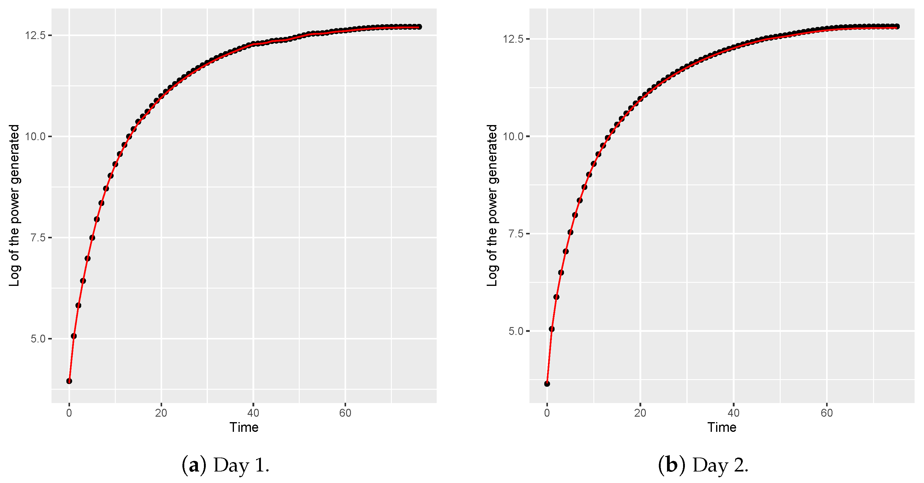
3.1. Fitted Model

The results of the fit of ten regression models using the dataset (Section 2.2) are presented in this section. The considered models are described in

Table 3. The considered models.

Model	Expression	Random Effect
$M_0$	$W_t={\beta }_0+{\beta }_1{I}_t+{\beta }_2{M}_t+{\epsilon }_t$	None
$M_1$	${\mathbb{Y}}_t={\alpha }_0-log\left(1+exp\{{\beta }_0-\gamma t\}\right)+{\epsilon }_t$	None
$M_2$	${\mathbb{Y}}_t=({\alpha }_0+A_t)-log\left(1+exp\{{\beta }_0-\gamma t\}\right)+{\epsilon }_t$	$a_t\sim \mathcal{N}(0,{\sigma }_a^2)$
$M_3$	${\mathbb{Y}}_t={\alpha }_0-log\left(1+exp\{({\beta }_0+B_t)-\gamma t\}\right)+{\epsilon }_t$	$b_t\sim \mathcal{N}(0,{\sigma }_b^2)$
$M_4$	${\mathbb{Y}}_t={\alpha }_0-log\left(1+exp\{{\beta }_0-(\gamma +C_t)t\}\right)+{\epsilon }_t$	$c_t\sim \mathcal{N}(0,{\sigma }_c^2)$
$M_5$	${\mathbb{Y}}_t=({\alpha }_0+A_t)-log\left(1+exp\{({\beta }_0+B_t)-\gamma t\}\right)+{\epsilon }_t$	$(a_t,b_t)\sim {\mathcal{N}}_2\left(\left(\begin{array}{c}0\\ 0\end{array}\right),\left[\begin{array}{cc}{\sigma }_a^2& 0\\ 0& {\sigma }_b^2\end{array}\right]\right)$
$M_6$	${\mathbb{Y}}_t=({\alpha }_0+A_t)-log\left(1+exp\{{\beta }_0-(\gamma +C_t)t\}\right)+{\epsilon }_t$	$(a_t,c_t)\sim {\mathcal{N}}_2\left(\left(\begin{array}{c}0\\ 0\end{array}\right),\left[\begin{array}{cc}{\sigma }_a^2& 0\\ 0& {\sigma }_c^2\end{array}\right]\right)$
$M_7$	${\mathbb{Y}}_t={\alpha }_0-log\left(1+exp\{({\beta }_0+B_t)-(\gamma +C_t)t\}\right)+{\epsilon }_t$	$(b_t,c_t)\sim {\mathcal{N}}_2\left(\left(\begin{array}{c}0\\ 0\end{array}\right),\left[\begin{array}{cc}{\sigma }_b^2& 0\\ 0& {\sigma }_c^2\end{array}\right]\right)$
$M_8$	${\mathbb{Y}}_t=({\alpha }_0+A_t)-log\left(1+exp\{({\beta }_0+B_t)-(\gamma +C_t)t\}\right)+{\epsilon }_t$	$(a_t,b_t,c_t)\sim {\mathcal{N}}_3\left(\left(\begin{array}{c}0\\ 0\\ 0\end{array}\right),\left[\begin{array}{ccc}{\sigma }_a^2& 0& 0\\ 0& {\sigma }_b^2& 0\\ 0& 0& {\sigma }_c^2\end{array}\right]\right)$
$M_9$	Equation (8)	See Equation (6)

, where $A_t$ and $B_t$ are given by Equation (6) and $C_t={\gamma }_1{\mathbb{Z}}_t+{\gamma }_2{M}_t+c_t$ for $c_t\sim \mathcal{N}(0,{\sigma }_c^2)$.

Model $M_0$ was a linear predictor and model $M_1$ was given by the log-logistic function in Equation (5). Models $M_2$, $M_3$ and $M_4$ were given by log-logistic functions with random effects in just one parameter. Models $M_5$, $M_6$ and $M_7$ were given by log-logistic functions with random effects in two parameters. Model $M_8$ was given by a log-logistic function with random effects in three parameters. Opposite to the proposed model that was described in Equation (8), models $M_2$ to $M_8$ considered that the random effects were independent from one another and that the random errors were not correlated. Hereafter, we call the proposed model $M_9$.

In order to obtain estimates for the parameters of models $M_1$ to $M_8$, we used the R software [27] and the nlme command [28]. To obtain estimates for the parameters of model $M_9$, we included the options $correlation=corAR1\left(\right)$ and $weights=varPower\left(\right)$ in the nlme command. The fitted models were compared using the mean squared error (MSE) and the AIC and BIC selection criteria metrics. The best model was the one that had the lowest values for the MSE, AIC and BIC.

Table 4. The values for the selection criteria of the models.

Criteria	Model
	${\mathit{M}}_{\mathbf{0}}$	${\mathit{M}}_{\mathbf{1}}$	${\mathit{M}}_{\mathbf{2}}$	${\mathit{M}}_{\mathbf{3}}$	${\mathit{M}}_{\mathbf{4}}$	${\mathit{M}}_{\mathbf{5}}$	${\mathit{M}}_{\mathbf{6}}$	${\mathit{M}}_{\mathbf{7}}$	${\mathit{M}}_{\mathbf{8}}$	${\mathit{M}}_{\mathbf{9}}$
MSE	0.0037	0.3334	0.2181	0.2998	0.2338	0.2056	0.218	0.2119	0.1889	0.0007
AIC	−4495.575	2834.605	2245.463	2730.587	2351.410	2191.774	2248.816	2234.820	2090.743	−15,395.292
BIC	−4474.002	2856.177	2272.429	2757.554	2378.466	2229.527	2286.569	2272.573	2144.675	−15,325.179

shows the MSE values and the comparison criteria for the ten ($M_0-M_9$) fitted models. The smallest values are highlighted in bold. As can be seen from the table, the three criteria indicated that the proposed model ($M_9$) was the best.

Table 5. The estimates for the fixed parameters of model $M_9$.

Parameter	Estimate	Std. Error	DF	t-Value	p-Value
${\alpha }_0$	6.7092	0.2823	1598	23.7691	0.0000
${\alpha }_1$	0.6577	0.0210	1598	31.3600	0.0000
${\alpha }_2$	0.0696	0.0383	1598	1.8162	0.0695
${\beta }_0$	4.9754	0.2696	1598	18.4537	0.0000
${\beta }_1$	−0.4143	0.0162	1598	−25.6015	0.0000
${\beta }_2$	0.1148	0.0549	1598	2.0936	0.0365
$\gamma$	0.0009	0.0001	1598	9.4311	0.0000

shows the estimates for the fixed parameters of model $M_9$. A significance level of $\omega =0.10$ was used for the explanatory variables of irradiance and accumulated mass for this model. Since ${\beta }_2>0$ (the coefficient of variable M), the accumulated mass had a negative effect on the growth of the curve. By increasing M, the slope of the curve reduced, indicating a slower growth and, consequently, a smaller amount of generated solar power. Since ${\beta }_1<0$ (the coefficient of variable $\mathbb{Z}$) indicated that when the irradiance value increased, the slope of the curve increased, this meant that more solar power was generated.

Therefore, the fitted model was given by:

$${\widehat{\mathbb{Y}}}_t=6.7092+0.6577{\mathbb{Z}}_t+0.0696M_t-log(1+exp\{4.9754-0.4143{\mathbb{Z}}_t+0.1148M_t-0.0009t\})$$

(9)

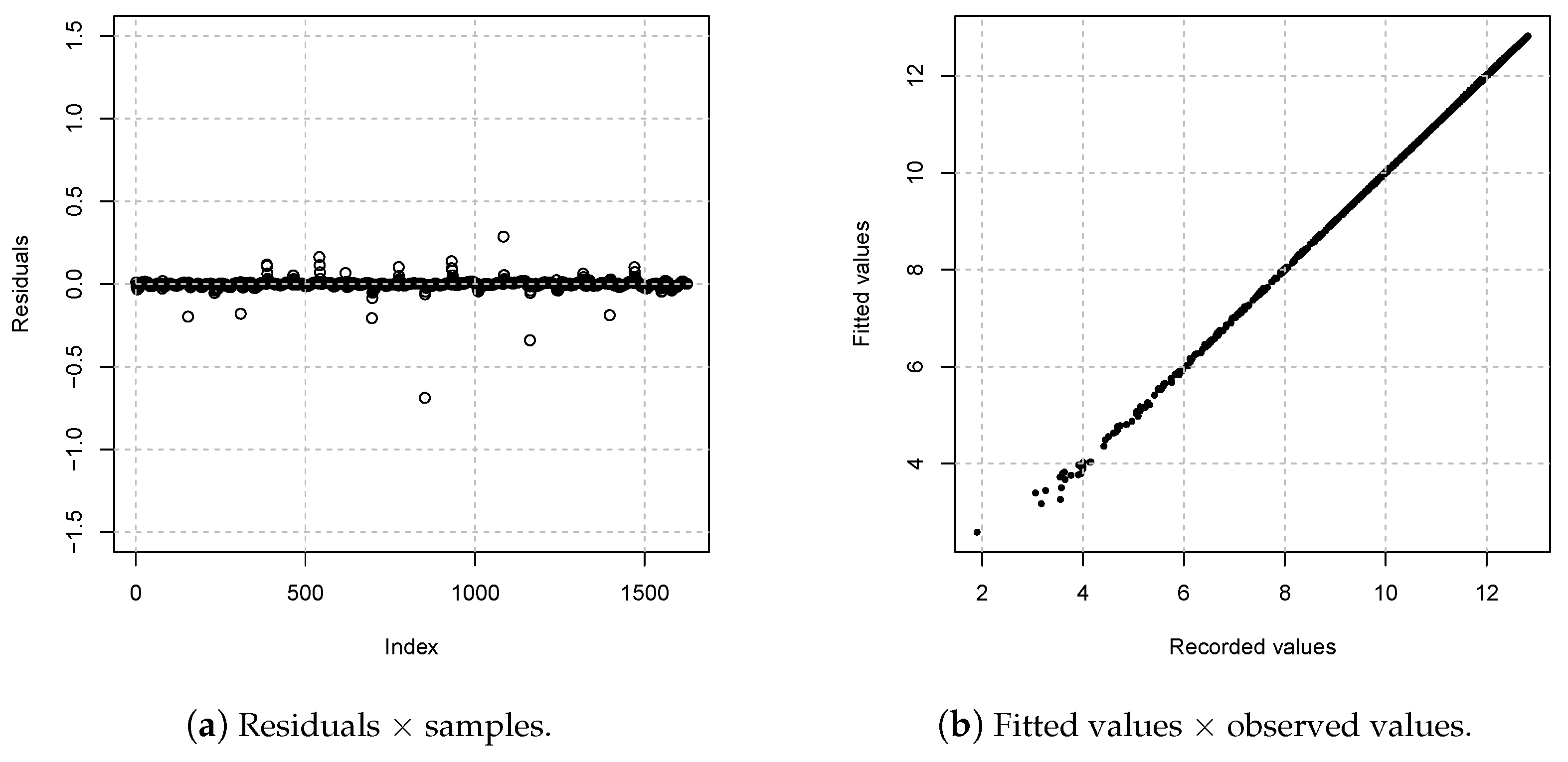
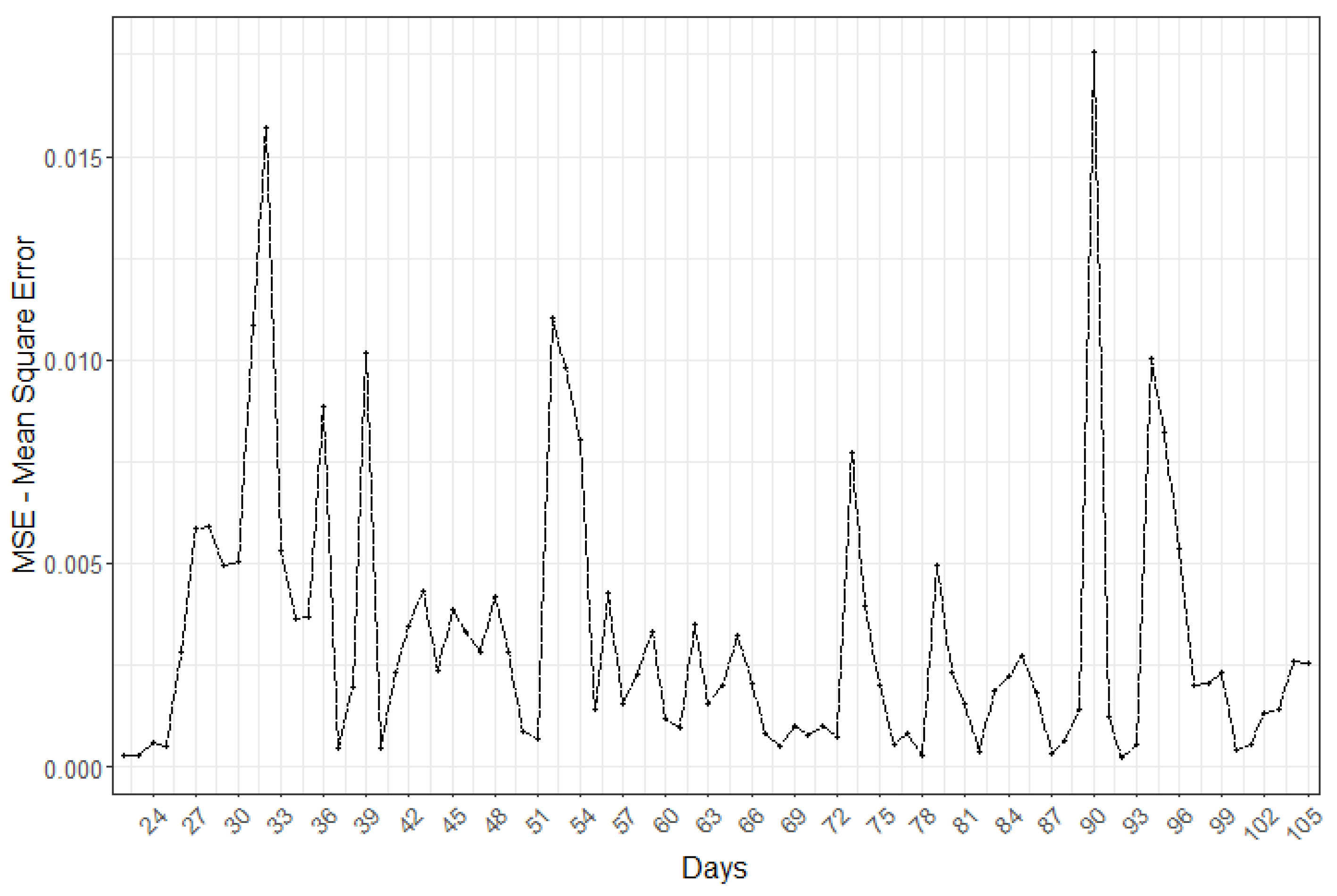
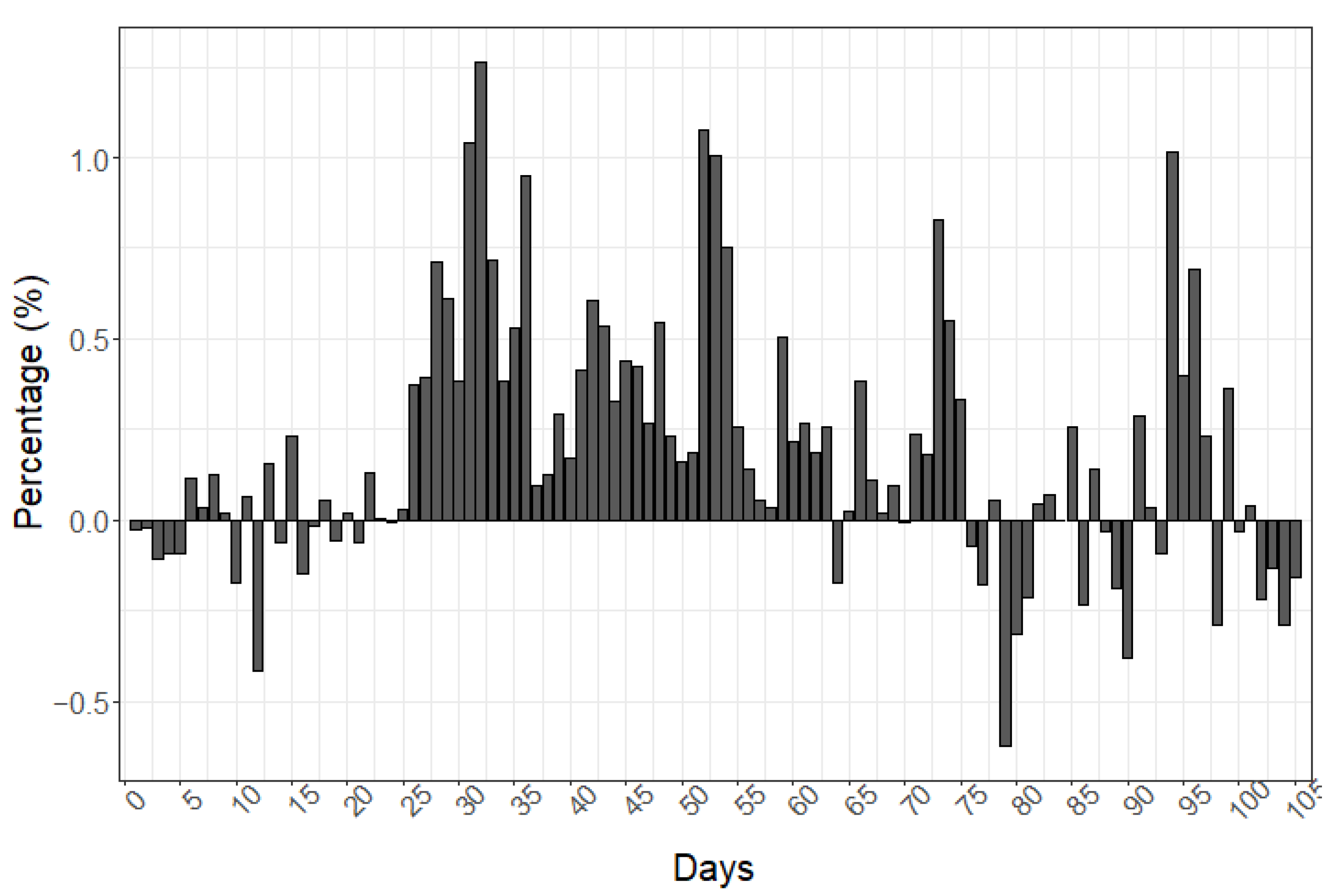
3.2. Model Validation

As the best fit model was the NLME model $M_5$, we validated the results by comparing the mean squared error (MSE) metric of the predicted and recorded (observed) values. In addition, the residuals of the model are also presented and discussed in this section. Figure 6 shows the observed values (• symbols) and the predicted values (red line) from days 1 and 2. The MSEs for days 1 and 2 were $0.00013$ and $0.00006$, respectively. Figure 7 shows the daily MSE for the first 21 days. During that period, the MSE ranged from $0.00006$ to $0.00613$, thus showing the high performance of the best fit model.

Figure 8 shows a plot of the residuals from samples (the first 21 days) from the dataset. It can be seen that all of the residuals were around 0 during the interval $(-1.0,0.5)$. Figure 8b highlights the close relationship between the fitted (predicted) and observed values. The linear correlation coefficient between the predicted and observed values was $0.9997$.

Regarding the model validation and the higher accuracy that was achieved by the NLME model for the samples from the first 21 days, the model was then evaluated using samples from the remaining 84 days. Figure 9 shows the daily MSEs from those 84 days, for which the values ranged from $0.00021$ to $0.01756$. The linear correlation coefficient between the predicted and observed values was $0.9996$, indicating that the model had a high performance and a fairly similar correlation to that from the testing period.

It can be seen that the environmental variables could impact the accuracy of the model. Figure 10 presents the rainfall precipitation levels and particle concentrations during the validation and evaluation period (105 days). A higher rainfall precipitation level had a straight effect on the particle concentrations in the air. This effect made it possible to correlate soiling on the PV modules to the effects of natural clean-up (rainfall). It is worth noting that the high precipitation levels between the months of November and March could explain the lack of accuracy (see the MSE peaks in Figure 7 and Figure 9) of the model.

Figure 11 presents the log of the daily observed and predicted generated power values from the 105 days. The model could closely capture the daily differences between the generated solar power values. The presence of high precipitation levels could mostly explain the lack of accuracy during this period.

The instability of the power generation (high and low values) throughout this period was due to cloudy conditions at the location of the PV system (mainly before and after rainfall). As rainfall became sparser (from March), the differences between the predicted and observed generated power values became more significant due to an increase in soiling deposition on the PV modules.

Another way to evaluate the performance of the proposed prediction model was to look at the percentage error of the generated power. Equation (10) represents the daily percentage power difference between the recorded and predicted values:

$$P_d=\left(\frac{O_d-E_d}{E_d}\right)\times 100,$$

(10)

where $O_d=exp\left\{{\mathbb{Y}}_{n_d}\right\}$ and $E_d=exp\left\{{\widehat{\mathbb{Y}}}_{n_d}\right\}$ for $d=1,\dots ,D=105$.

When $P_d<0$, the recorded generated power on the d-th day is less than the predicted (expected) generated power, meaning that soiling could be impacting power generation on that day. Engineers who are responsible for PV plants should also be aware that there could be electrical failures in the PV system. A value of $P_d>0$ means that the recorded generated power is higher than the predicted generated power. The reason for a positive difference could be that there is less soiling on the PV modules than estimated by the prediction model. This behavior could be associated with the natural clean-up of the modules in the PV array due to rainfall. PV system users should also pay attention when $P_d=0$ as this situation does not mean that there is no soiling on the modules, but rather that the predicted and observed values are quite similar. When $P_d=0$, users should observe whether the daily power generation curve is maintaining the same steady growth behavior or is slowing down (which could be evidence of soiling having an impact on power generation) over the given period.

Figure 12 shows the percentage differences from the 105 days. For the first 25 days, negative daily $P_d$ values were observed. Between days 25 and 60, there were only positive $P_d$ values. It can be seen in Figure 10 that these positive $P_d$ values could be associated with the high rainfall precipitation levels from November 2019 to March 2020. This behavior corroborated previous explanations of the effects of regular rainfall being responsible for the clean-up of PV modules. Since the model noticed the increase in accumulated mass over time but did not consider natural clean-up procedures (from rainfall), this explains why the predicted values were below the observed values (less than $1.4\%$). After the 80th day, negative values became more frequent, thus indicating an increase in soiling on the PV modules.

The correlation coefficient that was found for the model was $r=0.9999$ for the training set and $r=0.9996$ for the testing set. The mean squared error (MSE) significantly increased from the training set (MSE = 0.0007) to the testing set (MSE = 0.0032). The test period had more days with low and high precipitation rates, which impacted the forecasting accuracy. The fitted model was evaluated continuously over the period and obtained an overall MSE of 0.0027. The model could have achieved a better accuracy if restart points (i.e., on the d-th day, the model restarts the measurement of the accumulated mass of particles) had been performed just after days with a high precipitation rate. For example, by assuming a minimum threshold of 30 mm of rain precipitation as a restart point for the measurement of the mass accumulation of particles throughout the test period, the MSE decreased to $0.0028$ and the overall MSE was 0.0024.

4. Conclusions

This work presented a new nonlinear mixed-effects (NLME) predictor that was based on a log-logistic function to estimate photovoltaic power generation in solar power plants. The predictor model was designed using irradiance and mass-independent particulates as the exploratory variables. The response variable was the generated power at the instant of time t.

We evaluated ten different statistical predictors, among which the log-logistic model $\left(M_9\right)$ achieved the best values according to the AIC, BIC and MSE metrics. The predictor was then validated and evaluated using a dataset comprising environmental and PV power samples that were collected across 105 days (from October 2019 to April 2020) at a photovoltaic power plant in Campo Grande-MS, Brazil. The model was trained using the first 21 days from the sample data and the testing set comprised the remaining 84 days. From a practical viewpoint, the results showed that modeling the log-transformed power using a log-logistic model with fixed and random effects was very accurate for predicting power generation in the presence of soiling. To the best of our knowledge, this is the first work to propose the statistical modeling of power generation in PV plants based on a nonlinear mixed-effects model.

The proposed predictor could be widely applied in real large-scale environments to provide accurate generated power estimates and work together with other monitoring tools to track the performance of PV systems. The hardware infrastructure of the predictor is very simple (irradiance and soiling sensors) and most PV plants have standard weather or solarimetric stations from which irradiance and other environmental data are available.

It can be seen that the predictor uses accumulative input data to estimate power generation. During different events at the PV power plant site (e.g., maintenance procedures) or even under certain environmental conditions (e.g., high rainfall precipitation levels), the input variables may need to be restarted to cope with the new state of the PV system performance. Another useful advantage of the proposed predictor system is that users may obtain power generation estimates for short time intervals (hourly power generation) or large time intervals, for instance, at the end of the day (daily power generation).

The predictor behavior provided insights into the best time to perform clean-up procedures on PV arrays. A correct cleaning schedule for PV modules avoids unnecessary maintenance costs and maximizes profits by allowing the PV system to work at full capacity.

Some opportunities for future work include applying the model to a larger period, thus evaluating the power estimates under different weather conditions and seasons. Another subject for further research is the analysis of the thresholds for the training and testing sets to avoid model overfitting. Other targets for future work include applying the model to photovoltaic power plants with different module technologies or different soiling detection sources, such as images from cameras and satellites, and the use of machine learning models to estimate soiling on PV arrays.

References

1. Catelani, M.; Ciani, L.; Cristaldi, L.; Faifer, M.; Lazzaroni, M.; Rossi, M. Characterization of photovoltaic panels: The effects of dust. In Proceedings of the IEEE International Energy Conference and Exhibition, Florence, Italy, 9–12 September 2012; pp. 45–50. [Google Scholar]
2. Viana, T.; Rüther, R.; Martins, F.; Pereira, E. Assessing the potential of concentrating solar photovoltaic generation in Brazil with satellite-derived direct normal irradiation. Sol. Energy 2011, 85, 486–495. [Google Scholar] [CrossRef]
3. Asmelash, E.; Prakash, G.; Kadir, M. Webinar Series—Wind and Solar PV—What We Need by 2050. 2020. Available online: https://bit.ly/3LJJ63r (accessed on 17 October 2021).
4. Ribeiro, K.; Santos, R.; Saraiva, E.; Rajagopal, R. A Statistical Methodology to Estimate Soiling Losses on Photovoltaic Solar Plants. J. Sol. Energy Eng. 2021, 143, 064501. [Google Scholar] [CrossRef]
5. Hickel, B.M.; Deschamps, E.M.; Nascimento, L.; Rüther, R.; Simões, G.C. Análise da Influência do Acúmulo de Sujeira Sobre Diferentes Tecnologias de módulos FV: Revisão e medições de campo. In Proceedings of the VI Congresso Brasileiro de Energia Solar, Belo Horizonte, Brazil, 4–7 April 2016. [Google Scholar]
6. Zorrilla-Casanova, J.; Philiougine, M.; Carretero, J.; Bernaola, P.; Carpena, P.; Mora-López, L.; Sidrach-de Cardona, M. Analysis of dust losses in photovoltaic modules. In Proceedings of the World Renewable Energy Congress, Linköping, Sweden, 8–13 May 2011; pp. 8–13. [Google Scholar]
7. Dunn, L. PV module soiling measurement uncertainty analysis. In Proceedings of the 39th Photovoltaic Specialists Conference (PVSC), Tampa, FL, USA, 16–21 June 2013; pp. 658–663. [Google Scholar]
8. Sinha, P.; Hayes, W.; Littmann, B.; Ngan, L.; Znaidi, R. Environmental variables affecting solar photovoltaic energy generation in Morocco. In Proceedings of the 2014 International Renewable and Sustainable Energy Conference (IRSEC), Ouarzazate, Morocco, 17–19 October 2014; pp. 230–234. [Google Scholar]
9. Fernández-Solas, Á.; Montes-Romero, J.; Micheli, L.; Almonacid, F.; Fernández, E.F. Estimation of soiling losses in photovoltaic modules of different technologies through analytical methods. Energy 2022, 244, 123173. [Google Scholar] [CrossRef]
10. Zsiborács, H.; Zentkó, L.; Pintér, G.; Vincze, A.; Baranyai, N.H. Assessing shading losses of photovoltaic power plants based on string data. Energy Rep. 2021, 7, 3400–3409. [Google Scholar] [CrossRef]
11. de Oliveira, A.K.V.; Aghaei, M.; Rüther, R. Automatic Inspection of Photovoltaic Power Plants Using Aerial Infrared Thermography: A Review. Energies 2022, 15, 2055. [Google Scholar] [CrossRef]
12. Mehta, S.; Azad, A.P.; Chemmengath, S.A.; Raykar, V.; Kalyanaraman, S. DeepSolarEye: Power Loss Prediction and Weakly Supervised Soiling Localization via Fully Convolutional Networks for Solar Panels. In Proceedings of the 2018 IEEE Winter Conference on Applications of Computer Vision (WACV), Lake Tahoe, NV, USA, 12–15 March 2018; pp. 333–342. [Google Scholar]
13. García Márquez, F.P.; Segovia Ramírez, I. Condition monitoring system for solar power plants with radiometric and thermographic sensors embedded in unmanned aerial vehicles. Measurement 2019, 139, 152–162. [Google Scholar] [CrossRef]
14. Herraiz, Á.H.; Marugán, A.P.; Márquez, F.P.G. Photovoltaic plant condition monitoring using thermal images analysis by convolutional neural network-based structure. Renew. Energy 2020, 153, 334–348. [Google Scholar] [CrossRef]
15. Pavan, A.M.; Mellit, A.; De Pieri, D.; Kalogirou, S.A. A comparison between BNN and regression polynomial methods for the evaluation of the effect of soiling in large scale photovoltaic plants. Appl. Energy 2013, 108, 392–401. [Google Scholar] [CrossRef]
16. Pavan, A.M.; Mellit, A.; De Pieri, D. The effect of soiling on energy production for large-scale photovoltaic plants. Sol. Energy 2011, 85, 1128–1136. [Google Scholar] [CrossRef]
17. Javed, W.; Guo, B.; Figgis, B. Modeling of photovoltaic soiling loss as a function of environmental variables. Sol. Energy 2017, 157, 397–407. [Google Scholar] [CrossRef]
18. Hammad, B.; Al-Abed, M.; Al-Ghandoor, A.; Al-Sardeah, A.; Al-Bashir, A. Modeling and analysis of dust and temperature effects on photovoltaic systems’ performance and optimal cleaning frequency: Jordan case study. Renew. Sustain. Energy Rev. 2018, 82, 2218–2234. [Google Scholar] [CrossRef]
19. Al Siyabi, I.; Al Mayasi, A.; Al Shukaili, A.; Khanna, S. Effect of soiling on solar photovoltaic performance under desert climatic conditions. Energies 2021, 14, 659. [Google Scholar] [CrossRef]
20. Lindstrom, M.J.; Bates, D.M. Newton—Raphson and EM algorithms for linear mixed-effects models for repeated-measures data. J. Am. Stat. Assoc. 1988, 83, 1014–1022. [Google Scholar]
21. El-Shobokshy, M.S.; Hussein, F.M. Effect of dust with different physical properties on the performance of photovoltaic cells. Sol. Energy 1993, 51, 505–511. [Google Scholar] [CrossRef]
22. Hupa, L.; Bergman, R.; Fröberg, L.; Vane-Tempest, S.; Hupa, M.; Kronberg, T.; Pesonen-Leinonen, E.; Sjöberg, A.M. Chemical resistance and cleanability of glazed surfaces. Surf. Sci. 2005, 584, 113–118. [Google Scholar] [CrossRef]
23. Coello, M.; Boyle, L. Simple model for predicting time series soiling of photovoltaic panels. IEEE J. Photovolt. 2019, 9, 1382–1387. [Google Scholar] [CrossRef]
24. Blumberg, A. Logistic growth rate functions. J. Theor. Biol. 1968, 21, 42–44. [Google Scholar] [CrossRef]
25. Davidian, M.; Giltinan, D.M. Nonlinear Models for Repeated Measurement Sdata; CRC Press: Boca Raton, FL, USA, 1995; Volume 62. [Google Scholar]
26. Xu, P.; Shen, Y.; Fukuda, Y.; Liu, Y. Variance component estimation in linear inverse ill-posed models. J. Geod. 2006, 80, 69–81. [Google Scholar] [CrossRef]
27. R Core Team. R: A Language and Environment for Statistical Computing; R Foundation for Statistical Computing: Vienna, Austria, 2021. [Google Scholar]
28. R Core Team. nlme: Linear and Nonlinear Mixed Effects Models. R Package Version 3.1-141. 2019. Available online: http://CRAN.R-Project.Org/Package=Nlme (accessed on 6 April 2022).
Figure 1. The PM1.0 particle concentration in the air, as recorded by the SPS30 sensor (19 April 2020).
Energies 15 05973 g001
Figure 2. The particle masses and concentrations from October 2019 to April 2020.
Energies 15 05973 g002
Figure 3. The weekly particle concentration averages (#/ cm 3 ).
Energies 15 05973 g003
Figure 4. The generated power (kW), temperature (Celsius) and irradiance (kW/ m 2 ) measurements in the log scale and the values of the accumulated mass of particles (μg/ c m 3 ).
Energies 15 05973 g004
Figure 5. The generated solar power on day 1.
Energies 15 05973 g005
Figure 6. The recorded and predicted values.
Energies 15 05973 g006
Figure 7. The MSE values for the first 21 days.
Energies 15 05973 g007
Figure 8. The residuals and the fitted values.
Energies 15 05973 g008
Figure 9. The daily MSEs from days 22 to 105.
Energies 15 05973 g009
Figure 10. The concentration of suspended particles in the and the rainfall precipitation levels from October 2019 to April 2020.
Energies 15 05973 g010
Figure 11. The total predicted (blue) and observed (red) generated power values from October 2019 to April 2020.
Energies 15 05973 g011
Figure 12. The percentage differences across the period.
Energies 15 05973 g012