Electricity Spot Price Modeling and Forecasting in European Markets

Abstract

In many competitive electricity markets around the world, the dynamic behavior of hourly electricity prices is subject to significant uncertainty and volatility due to electricity demand, availability of generation sources, fuel costs, and power plant availability. This work is devoted to describing and comparing the dynamics of electricity prices for some markets in Europe, selecting the five countries representing the largest economies in Western Europe (France, Germany, Italy, Spain, and the United Kingdom). Additionally, Denmark is included in the study to assess whether the size of the country is a determinant of price behavior. The six datasets of hourly price series, which exhibits a strong daily seasonality, are modelled using the most relevant well-known statistical models for time series analysis: ARIMA models and different versions of GARCH models. The comparison of the estimated models’ parameters, the analysis of outliers’ rate of appearance and the evaluation of out-of-sample one-day-ahead forecast let us draw some insightful similarities and dissimilarities between the analyzed countries.

1. Introduction

1.1. Motivation

Electricity markets have experienced a significant transformation around the world in the last few decades. The price of electricity set by the government each year is entirely determined by the market every day. In most countries, the price of electricity is arranged through a daily auction for each 24 h of the next day. The results of the daily market, based on free contracting between buying and selling agents, represent an efficient solution from the economic point of view but introduce huge uncertainty for the market participants: producers, sellers, and consumers.

In the European Union, the wholesale electricity market operates under the so-called “uniform price” rule [1,2]. In summary, the uniform pricing procedure is as follows: The daily demand is first satisfied by the supply of technologies whose production costs are lower, allowing them to offer electricity at a lower price. In practice, these technologies are those that produce non-storable electricity, such as nuclear and renewables. If this supply is insufficient to meet the total demand, the unsatisfied part of the demand is covered by the technology from among all the others whose offered prices are lower, and so on. The final price is the price corresponding to the supply that satisfies the last fraction of demand. This final price is largely related to the production costs of the most expensive technology entering the market supply. In this pricing system, all technologies are remunerated at the matching price, resulting in benefits of considerable magnitude for those technologies that generate electricity at a lower cost.

Distinct from most financial or commodity markets, the electricity “spot market” is typically a daily market that does not allow continuous trading. This is because system operators require advance notice to verify that the schedule is feasible and conforms to transmission constraints. These deregulated prices have been characterized in all the markets by having extremely high volatility.

Several elements explain the high volatility observed in electricity prices [3]. Probably the most important factor is the impossibility of storing electricity. Electricity cannot be physically stored directly, and production and consumption must be continuously balanced. Therefore, supply and demand shocks cannot be smoothed easily and directly affect equilibrium prices. Demand and supply characteristics also play an essential role in the observed volatility. The electricity demand is highly inelastic because it is a necessary good and highly dependent on weather conditions. The characteristics of the supply pool in each market can also contribute to the volatility of a given demand. The relative insensitivity of demand to price fluctuations and supply constraints at peak times make short-term electricity prices extremely volatile. Therefore, in markets where demand and supply curves are steep, we can observe sharp price increases as the quantity demanded increases. Moreover, depending on the structure of the market and the market power of generators, for high levels of demand, only a few generators could satisfy the residual demand and, therefore, market power could come into play through monopolistic or oligopolistic behavior of generators.

Most wholesale electricity markets use the “new” uniform auction system to set the price. However, the recent experience and perceived poor performance of some decentralized electricity markets has led some regulators to “revisit” the adoption of discriminatory or “pay-as-you-bid” auctions. Under this rule, each market participant is remunerated according to the price of its bid. In the short term, less is paid for electricity, but clean energy is no longer incentivized. It is well known that discriminatory auctions are not usually superior to uniform auctions in the medium and long term [2,4]. Both types of auctions are commonly used in financial and other markets, and there is now a voluminous economic literature devoted to their study. The system of “pay-as-you-bid” or discriminatory auctions resembles the old system of market operation prior to the liberalization of the electricity sector.

There is currently an intense debate in the European electricity sector about the best pricing system. Critics of the uniform auction system argue that some large utilities have the market power to artificially alter prices. The aim of our article is to statistically describe how electricity prices evolve in six countries using the uniform auction system. This comparative study may be useful to help policy makers and market players evaluate the current pricing system in the European Union.

As mentioned above, uniform pricing mechanism introduces huge uncertainty, which means the economic risk for the agents involved in the market. Logically, it is beneficial for any participant in the auctions to have a procedure for predicting prices when configuring their purchase or sale bids. Given the importance of electricity prices in a country’s economy [5], the prediction problem has been the subject of an enormous research effort from the electricity companies with the support of specialists in statistics and finance from around the world. The statistical analysis performed and the models constructed allow us to answer another question of special interest, which is to quantify the uncertainty associated with the price prediction in each country.

1.2. Aim

This paper aims to statistical analyze hourly electricity price series in six European countries: Denmark, France, Germany, Italy, Spain, and the United Kingdom, using time series models. The purpose of the analysis is to select a procedure to make predictions for the next day’s 24-h prices. With the help of the selected models, the prices predictability for each country is compared. The five most prominent countries in the European Union have been selected with Denmark.

1.3. Literature Review

A significant number of references have been devoted to the electricity price forecasting in the state-of-the-art technical literature [6,7,8]. In general terms, the proposed techniques can be grouped into three categories in accordance with the forecasting framework: statistical models, time series methods and artificial intelligence.

Concerning the time series approach, in the last years some studies have addressed the electricity price forecasting using a hybrid approach of statistical and regression models, based on a NARMAX model [9], or ARMAX Models based on a linear regression where functional parameters operate on functional variables [10]. Other references employ dynamic trees and random forest statistical techniques [11].

Concerning the artificial intelligence area, in the last years some references have analyzed the techniques based on deep learning on hybrid platform [12], ensemble learning [13], parametric and non-parametric approaches such as nonparametric and/or functional AR models [14], Hybrid ANN and Artificial Cooperative Search Algorithm [15], General Regression Neural Network and Harmony Search Algorithm [16], via Hybrid Backtracking Search Algorithm and ANFIS Approach [17], and a comparative of different machine learning techniques such as random forest regressor models, deep neural networks, convolutional neural networks [18].

1.4. Contribution

The contribution of this paper is twofold. First, the hourly price series of six most-representative European electricity markets have been described and modelled using ARIMA models and different versions of GARCH models. Secondly, a set of similarities and differences has been drawn after the exhaustive comparison of the: (i) estimated ARIMA/GARCH parameters, (ii) outliers’ rate of appearance, and (iii) the evaluation of out-of-sample one-day-ahead forecasts.

1.5. Paper Organization

The rest of this paper is organized as follows. Section 2 describes the collection of data employed in this study. Section 3 and Section 4 model the daily price time series using ARIMA and GARCH techniques, respectively. Section 5 and Section 6 are devoted to analyzing the data asymmetry and comparing the out-of-sample forecasts accuracy, respectively. Finally, Section 7 provides some relevant conclusions. The analysis performed is summarized using the flow chart in Figure 1 below.

2. Electricity Prices Dataset

2.1. Characteristics

There is a very general agreement about listing the main characteristics observed in the descriptive analysis of the price series, which is common to practically all liberalized electricity markets. The first is the existence of jumps and spikes, which is justified by the difficulty of storing large quantities of energy to allow a smooth adjustment between supply and demand. The second is the strong seasonality due to the dependence of electricity demand on weather conditions and social and economic activities that generate daily, weekly, and annual cycles. Finally, another feature that is common to other financial markets is the existence of intense heteroskedasticity, which creates periods of high volatility [19,20,21].

2.2. Single Day-Ahead Coupling

Most of Europe is now part of the Single Day-Ahead Coupling (SDAC), which is a coordinated electricity price setting and cross-zonal capacity allocation mechanism that simultaneously matches orders from the day-ahead markets per bidding zone, respecting cross-zonal capacity, and allocation constraints between bidding zones. This allocates scarce cross-border transmission capacity efficiently by coupling wholesale electricity markets from different regions. It does so by simultaneously considering cross-border transmission constraints. Its goal is to create a single pan-European cross-zonal day-ahead power market. Every day of the year, at 12:00 CET, the daily market session takes place in which the prices and the volume of energy for the twenty-four hours of the following day are fixed in most European countries (Spain, Portugal, Germany, Austria, Belgium, Bulgaria, Croatia, Slovakia, Slovenia, Estonia, France, Holland, Hungary, Ireland, Italy, Latvia, Lithuania, Luxembourg, Finland, Sweden, Denmark, Norway, Poland, the United Kingdom, the Czech Republic, and Romania). The daily market (SDAC) aims to carry out electricity transactions by submitting bids for market players’ sales and purchase of electricity. For instance, buying and selling agents located in Spain or Portugal will submit their bids to the daily market through OMIE, which is the sole designated NEMO in those countries (NEMO stands for a Nominated Electricity Market Operator and they are the organizations mandated to run the day-ahead and intraday integrated electricity markets in the EU). Their buy and sell bids are accepted based on their economic merit order and the available interconnection capacity between the price zones. Suppose at a particular hour of the day, the interconnection capacity between two zones is sufficient to allow the flow of electricity resulting from the negotiation; in this case price of electricity at that hour will be the same in both zones if inverse, and at that hour the interconnection is fully occupied, at that time the pricing algorithm results in a different price in each zone. This described mechanism for electricity price formation is called market coupling.

The existence of the SDAC mechanism conditions the price dynamics of each national market, although the distances between countries and interconnection capacity restrictions, among other factors, cause the evolution of prices in many areas to vary independently.

2.3. Dataset

Hourly prices have been collected for six countries (Denmark, Germany, France, Italy, Spain, and the UK), starting 1 January 2013 and lasting until 31 December 2019. To see how the European daily market (SDAC) affects the prices of the different markets analyzed, provides the percentage of hours (corresponding to weekdays) in which there has been price coincidence in two countries in the sample. For example, during the study period, prices in France and Spain have coincided in 17.9% of the hours. Moreover, the highest percentage is for Denmark and Germany with 29.8%.

Another important feature of the dynamics of the hourly electricity price series is the strong seasonality. In many applications, the seasonal behavior can be perfectly described with stationary time series models. However, in this case, the strong seasonality is associated with a loss of stationarity, leading to periodic changes in the mean and correlation structure of the process. These types of processes are known as periodically correlated processes [21,22]. In their analysis of daily average prices, Koopman et al. [21] mentions the lack of stationarity of the series and recommend using different ARIMA models for each day of the week. Tiao and Grupe [23] explored the properties of periodic models to characterize seasonal time series. In their paper [23], the authors showed that the use of stationary ARMA models when processes are periodic leads to a loss in predictive accuracy. As a result of this, several authors prefer to predict hourly electricity prices with different models for weekdays and weekends [24,25]. All these considerations lead us to limit our analysis to working days (Monday to Friday), eliminating Saturdays and Sundays from the series.

This is a very critical aspect because it creates a discontinuity in the series. This decision, however, greatly simplifies the analysis of the series and focuses on the most relevant days in the price series. The left plot in Figure 2 shows the median prices for each of the 24-hourly series for each country; whereas the right plot shows the robust estimate of the standard deviation (median of the absolute deviations from the median, adjusted by a factor for asymptotically normal consistency) of the same series. Prices show a clear bimodal curve with two different hours in the day, which are markedly higher than neighboring values: these are hours between 8 and 10 a.m. and 6 and 10 p.m. In a comparative perspective across different European markets, data shows clearly that Italy has values structurally higher if compared with the other markets. Based on Figure 2, Spain has the second-highest median prices, followed by France and Germany. The median price curves for Denmark and the UK are similar for the first half of the day and higher in the UK for the second half. Denmark and the UK have lower average prices in most hours than the other countries. The price differences among countries are very considerable, e.g., Italy has average values 50 to 80% higher than Denmark.

Concerning the variability changes according to the hours in the different countries (right plot of Figure 2): The differences are very pronounced in general for all countries except Spain. The fact that the variability is not constant is very relevant when choosing the model. This case indicates that the hourly price series does not have constant variance and is not stationary. Following the recommendation of Tiao and Grupe [23], the use of an ARIMA model for the hourly series is not appropriate.

Figure 3 shows the daily average price series (black-colored line) with the mean values and the standard deviation. The difference in level between the Italian series and the Danish or British series is observed. The existence of jumps and spikes, the lack of trend, and the reversion effect to the mean can be seen in all the graphs. The red-colored line depicts the smoothed series using Lowes. The value in parentheses below the standard deviation is the measure of the dispersion of the data against the smoothed curve (red). With respect to this indicator, the difference in behavior between the UK series and the others is very striking.

The evolution of average prices over seven years shows there is no trend in any of the series. The graphs for some countries show strong similarities, e.g., Denmark and Germany. Furthermore, Italy and France, especially from 2016 onwards. The degree of similarity can be measured by the correlation matrix or by the correlation matrix of the differenced series (

Table 1. The correlation matrix of the differenced series.

	Den	Fra	Ger	Ita	Spa	UK
Den	1	0.360651	0.781651	0.034087	−0.05867	0.388412
Fra	0.360651	1	0.175669	0.712271	0.361348	0.61889
Ger	0.781651	0.17567	1	0.078789	−0.08945	0.276344
Ita	0.034087	0.712271	0.078789	1	0.525755	0.457873
Spa	−0.05867	0.361348	−0.08945	0.525755	1	0.100781
UK	0.388412	0.61889	0.276344	0.457873	0.100781	1

). The correlation between Denmark and Germany is high for both average and incremental data. It is also high for the pairs (Denmark, UK), (France, Italy) and (France, UK).

3. ARIMA Models and Outliers

The literature on modeling and analyzing electricity prices is abundant and growing quickly. Most of the initial literature is in the finance area and focuses on developing realistic spot price models, analytically tractable for the purposes of derivative pricing and risk management. During recent decades, many statistical techniques and models have been developed for forecasting whole-sale electricity prices, especially for short-term price forecasting. The complexity of electricity price dynamics can be seen in [21], One of the most complete studies on the subject. Weron [8] presents an extensive review of the established approaches to modeling and forecasting electricity prices [8]. A variety of methods and ideas have been tried for electricity price forecasting, with varying degrees of success. The review article aims to explain the complexity of the available solutions, with a special emphasis on the strengths and weaknesses of the individual methods.

This and many other articles summarize the factors influencing price behavior and compare different approaches, such as Artificial Neural Networks, Auto Regressive Integrated Moving Average Models, dynamic regressions, Support Vector Machine models, Wavelets, and methods that combine different models. Basically, the works conclude that time series models are the ones which generally provide better results [26,27].

Looking specifically at time series models, we can distinguish many different approaches in the literature. Hourly electricity prices for a country form a univariate time series. The natural approach is to initially analyze the complete hourly time series with an ARIMA model, including the different seasonalities present in the process. This is the starting point for many authors. A single ARIMA model is not sufficient for collecting all the peculiarities of price dynamics. Prof. Conejo et al. [26] use a different model for each season for the PJM Interconnections (Pennsylvania-New Jersey-Maryland). As we have anticipated in the previous sections, the time series is not stationary. The variance varies from one hour to another, the autocorrelation structure is different for different times of the day, and so on. Furthermore, and most important of all, this strategy provides predictions compared to the alternative of modeling each hour independently, the discussion and analysis carried out by [24]. In other words, the parameters associated with the dynamics of the process are different for each hour of the day. Tiao and Groupe [23] showed that the use of stationary ARMA models when processes are periodic leads to a loss in predictive accuracy. In the hourly price series, there is a clear periodicity of length 24. Therefore, the approach preferred by several authors, is to use different models for each of the 24 h in a day [24,25,28,29,30].

Gladyshev [31] proved that any periodic process could be written as a multivariate stationary process of dimension equal to the length of the period (24, in this case). This led some authors to pose the problem as a case of multivariate time series. However, in this case, the direct application of multivariate ARIMA models requires many parameters. For instance, the IMA(1,1), one of the simplest models, needs to estimate a 24 × 24 square matrix plus the 24 × 24 error covariance matrix. If the day-of-the-week seasonal effect is included, a new 24 × 24 matrix will be required, and the final multivariate model will accumulate a huge number of total parameters. Reducing the parameter space is essential for successfully modeling multivariate time series. The problem is solved in the time series literature by dimension reduction using dynamic factor models [24,32,33].

The univariate periodic correlated series analysis through multivariate models is seldom practical. For example, Carpio et al. [24] uses the multivariate exponential smoothing model, which requires in total 876 parameters. Two conclusions with very relevant practical implications stand out from this article [24]: the first one, as announced by Tiao and Grupe [23], not considering cyclostationarity and using a single stationary ARIMA model for the whole hourly series provides very bad predictions; second, as pointed out, there is an alternative to using a vector model, which is the use of 24 univariate models, one for each hour of the day. This alternative is much simpler and provides predictions in the same way as the multivariate model.

The previous paragraphs conclude that the best way to model the evolution of electricity prices is through 24 univariate models, one for each hour of the day.

Working with 24 models introduces some complexity to the problem, but a great advantage arises; each of the 24 models is very simple. Following the usual procedure in analyzing other commodity prices, we will use the logarithm of the price as the variable to be modeled. Standard analysis of each series using the Box-Jenkins methodology suggests the ARIMA (0,1,1) model as an acceptable model to capture the price dynamics. Thus, calling $y_{h,t}=\log (p_{h,t})$ with $p_{h,t}$ being the price of electricity for hour $h$ of day $t$, the model can be written as:

$$y_{h,t}=y_{h,t-1}+{\theta }_h{u}_{h,t-1}+u_{h,t},h=1,2,\dots ,24$$

(1)

where $u_{h,t}$ (with $h$ fixed) is a white noise process with variance ${\sigma }_h^2$ and ${\theta }_h$ is the model parameter to be estimated from the data.

3.1. Detection of Outliers

As previously mentioned, electricity prices often undergo sudden changes that affect the dynamics of the data on a transient basis. It is difficult in many cases to know the causes of these changes. Detecting and correcting for the effect of outliers is important because they impact model selection, parameter estimation and, consequently, forecasts. There are several well-known computer programs specialized in the automatic detection of outliers in time series, such as X-12-ARIMA (developed by the U.S. Census Bureau) and TRAMO (developed by the Bank of Spain) [34]. A procedure used to detect outliers in time series is available in the R package tsoutliers [35]. The following types of outliers are considered: AO, additive outliers; LS, level shifts; TC, temporary changes and SLS, seasonal level shifts. The tsoutliers package [35] implements the procedure developed by [36]. The outlier detection procedure has been applied to each of the 24-time series for each country.

The bar chart in Figure 4 shows the total number of outliers in each country (total in gray, downward in blue, upward in red). During the analyzed period, 7 years, the market with the least outliers is the German market (1.02%), and the market with the highest proportion of outliers is the Spanish market (4%). It is important to highlight the high proportion of days affected with outliers, 4 of the six countries analyzed have over 10% of the days with at least one outlier observation. Most outlier observations in Denmark, Germany, France, and Spain correspond to sharp price declines. In Italy and Great Britain, the proportion of outliers in both directions is similar. The number of outliers detected logically depends on the criteria used to declare an observation as an outlier. The number of outliers changes with different criteria, but the structure observed by country and time is very similar.

The complexity of predicting electricity prices can be deduced from the outlier analysis performed. The existence of outlier observations seriously affects the estimation of the model. Moreover, by their very definition, outliers are very difficult to predict. However, it is the critical issue of price-prediction models in many cases (especially in the Spanish case). Many papers [37,38,39,40] use explanatory variables, such as weather conditions, daily demand structure, and other factors to model and predict jumps in the price series. Although there have been attempts to predict the jumps, the results achieved so far are rather limited.

3.2. ARIMA Model Estimation

Once the outliers have been eliminated, the autocorrelation function and the partial autocorrelation function corresponding to the differentiated pricing log series of each hour in the markets studied show that univariate IMA (1,1) is a suitable model for all the hours. For a given hour, the optimal model (chosen following the usual model selection criteria) has a more complex structure but is only slightly better than the IMA (1,1) model.

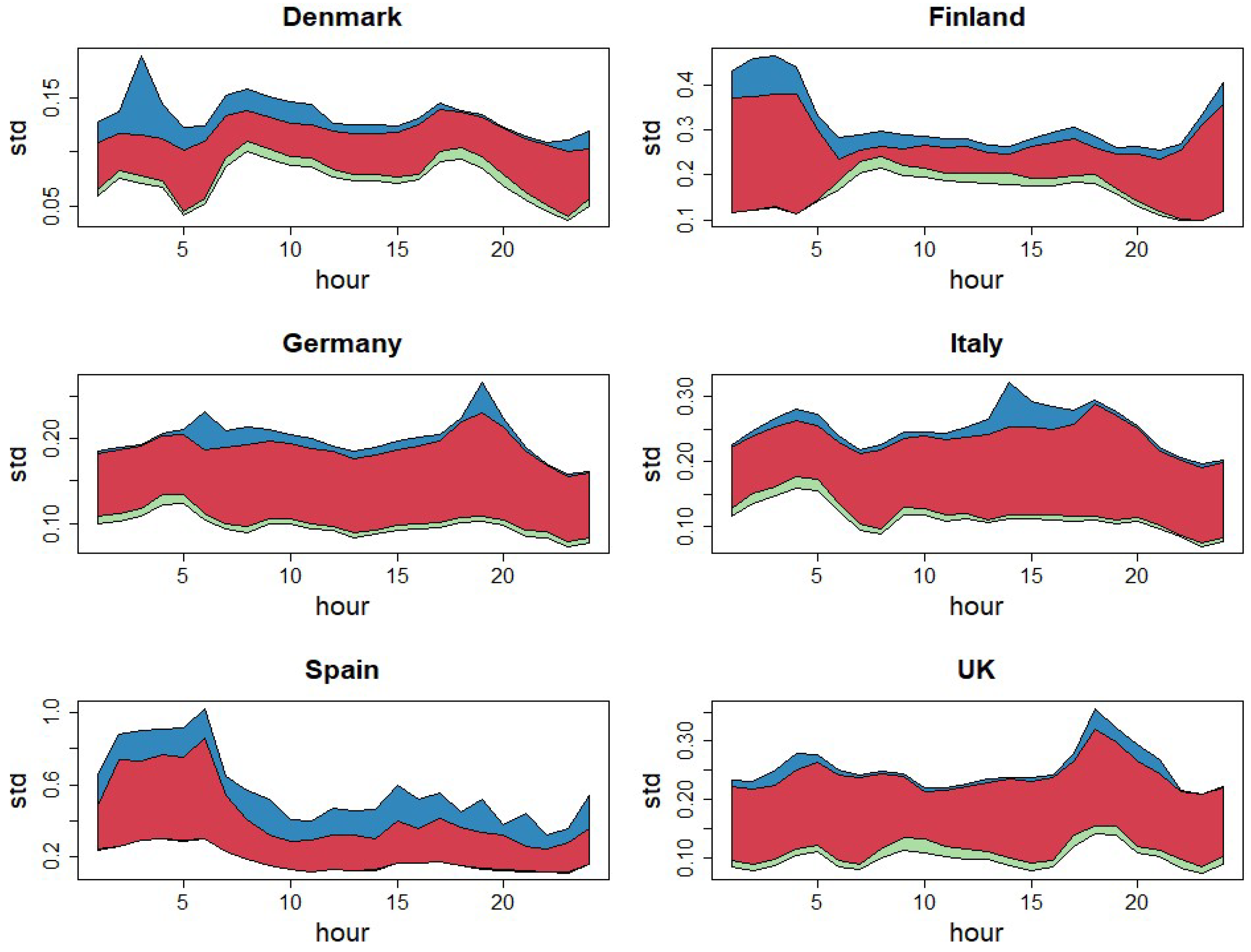
As a summary of the analysis performed using the ARIMA time series models, the graphs in Figure 5 are presented. A figure with four graphs (3 colors) is shown for each of the six countries studied. The top line shows the standard deviation of prices (in logarithms). This is the initial variability of each of the 24-time series. The series has been corrected by eliminating extreme values by analyzing and identifying outliers. The variability is logically reduced. The reduction in the standard deviation of the series due to the elimination of outliers is the blue band. The standard deviation for each hour of the corrected series is shown in the second line.

The corrected series is not stationary. Statistical analysis indicates that the main dynamics of prices largely correspond to the standard evolution of prices in other financial markets: the random walk. According to this model, the best prediction of the price of electricity for hour h of day t + 1 is to take the price observed for that hour on day t. If this prediction rule is used, the standard deviations of the prediction errors are shown in the third line (starting from the top). The reduction in standard deviation obtained after differentiation corresponds to the red band in Figure 5. The variability with respect to the second graph is very significantly reduced in all countries.

Finally, the lower graph shows the standard deviation of the ARIMA (0,1,1) model errors for each hour (exponential smoothing). The addition of the moving average parameter slightly improves the price predictions except for the Spanish case, where there is hardly any change concerning the random walk. The improvement in the models by including the moving average parameter is the light green band and is barely noticeable in Figure 5.

The graph can be interpreted as an analysis of the variance of the series. The most important component explaining the variability is the random walk (red band), outliers’ existence (blue band), and finally, the moving average parameter (green band).

Figure 6a shows the estimated standard deviations of the 24 models for each country. The standard deviations are quite stable at around 0.1 for Denmark, France, UK, and Italy. Germany has a higher variability of residuals than the previous four countries. The standard deviation of the first 6 h for Spain is much higher than the rest.

Figure 6b represents the estimations of the theta parameter of the IMA (1,1) model for each hour in the six markets. Denmark, UK, Italy, and France present highly significant theta estimates for all hours with values between 0.4 and 0.7. Germany shows theta values around 0.6 between 6 and 20 o’clock; outside this interval, the values are lower and unstable. The values of the theta parameter for Spain are very unstable, between −0.2 and 0.2, in many cases not significantly different from zero. The results observed in this graph are consistent with the sigma values represented in Figure 6a.

4. GARCH Models

4.1. Introduction GARCH Models

ARIMA models assume that the variance is constant over time. The evolution of $y_t=\mathsf{\Delta }\log \left(p_{h,t}\right)$ for the analyzed countries shows for all series there are periods with significant increases in variability. The variability or volatility of electricity prices is comparable to that of other financial markets (stock, bonds) or other commodities [1]. The deregulation has introduced new elements of uncertainty in the sector and therefore usual financial aspects such as financial risk management, derivative contracts, or hedging have been introduced in the industry. The variability bursts can be predicted with autoregressive models with conditional heteroscedasticity or ARCH models, initially introduced by [41] and extended by [42] to generalized ARCH or GARCH models.

There is no consensus in the literature on the most appropriate volatility model. According to [43], the optimal model depends on the forecasting horizon, and the country analyzed. As explained above, most studies differ from our approach in two aspects: they use daily average price data, and when they use hourly data, they do so with a single model for the 24 h of the day. Our interest in this paper is in day-ahead price predictions. This paper has studied the performance of six classes of ARMAX-GARCH volatility models (GARCH, eGARCH, gjrGARCH, apARCH, iGARCH, and cGARCH), and we have analyzed their behavior from the point of view of estimation and prediction.

The GARCH models combine two equations to explain the evolution of the variable of interest $y_{t }$, representing the logarithm of electricity price for an hour h of the day t. Equation (2) represents the ARIMA model of the variable $y_t$. In this case, we will use the ARIMA (0,1,1) or IMA (1,1) model, also known as exponential smoothing.

$$y_t=y_{t-1}+\theta u_{t-1}+u_t,t=1,2,\dots$$

(2)

where $u_t$ is a unbiased Gaussian-distributed random error and parameter $\theta$ is the IMA parameter to be estimated.

The innovations $u_t$ in Equation (2) is a sequence of random variables whose variance ${\sigma }_t^2$ is not constant. The second equation of the model, the GARCH equations, aims to explicitly model the time varying variance process. To simplify the explanation, we begin with the following GARCH (1,1) model:

$${\sigma }_t^2=\omega +\alpha u_{t-1}^2+\beta {\sigma }_{t-1}^2$$

(3)

where ω, α and β are the model parameters to be estimated from the data.

In this document, the term sGARCH refers to the previous model in Equation (3), standard GARCH. The three parameters of the model ω, α and β have to verify the following conditions: $\alpha \ge 0$, $\beta \ge 0$, $\alpha +\beta <1$ and $\omega >0$. The parameter $\alpha$ (the ARCH parameter) represents how volatility reacts to new information $u_{t-1}$, and $\beta$ (the GARCH effect) capture the degree of volatility persistence. The specification in Equation (2) is GARCH(1,1), but this can easily be extended to GARCH(p, q). The persistence is defined by $\widehat{P}=\alpha +\beta$ and ${\widehat{\sigma }}^2=\omega /\left(1-\widehat{P}\right)$ is unconditional variance. A particular case of this model is the integrated GARCH or iGARCH when $\alpha +\beta =1$.

When positive or negative shocks ($u_{t-1}$) have different impacts on volatility, the exponential GARCH (eGARCH) of [44] may be preferred:

$$\log \left({\sigma }_t^2\right)=\omega +\alpha +\gamma \left(\left|\frac{u_{t-1}}{{\sigma }_{t-1}}\right|-E\left|\frac{u_{t-1}}{{\sigma }_{t-1}}\right|\right)+\beta \log ({\sigma }_{t-1}^2)$$

(4)

where ω, α, $\gamma$ and β are the model eGARCH parameters to be estimated from the data. In addition to asymmetry, the eGARCH model in Equation (4) can also accommodate leverage, which is the negative correlation between returns shocks and subsequent shocks to volatility.

The gjrGARCH [45] models positive and negative shocks on the conditional variance asymmetrically using dummy variable $I_t$ that takes value 1 for $u_t<0$ and 0 otherwise:

$${\sigma }_t^2=\omega +\alpha u_{t-1}^2+\gamma I_{t-1}{u}_{t-1}^2+\beta {\sigma }_{t-1}^2$$

(5)

where ω, α, $\gamma$ and β are the model gjrGARCH parameters to be estimated from the data.

The variance exponent in Equation (5) is 2, some authors prefer to replace it by $\delta$ a new parameter that is estimated from the data, giving rise to the asymmetric power ARCH model (hereinafter referred as apARCH) of [46]:

$${\sigma }_t^{\delta }=\omega +\alpha {(\left|u_{t-1}\right|-\gamma u_{t-1})}^{\delta }+\beta {\sigma }_{t-1}^{\delta }$$

(6)

where $\delta >0$, and ω, α, $\gamma$, $\delta ,$ and β are the model parameters to be estimated.

The Component GARCH model of [47] decomposes the conditional variance into a permanent and transitory component. Letting $q_t$ represent the permanent component of the conditional variance, the model can be written as:

$${\sigma }_t^2=q_t+\alpha \left(u_{t-1}^2-q_{t-1}\right)+\beta \left({\sigma }_{t-1}^2-q_{t-1}\right)$$

(7)

$$q_t=\omega +\rho q_{t-1}+\varphi \left(u_{t-1}^2-{\sigma }_{t-1}^2\right)$$

(8)

where ω, α, β, $\rho$, and $\varphi$ are the model cGARCH parameters to be estimated from the data.

Results

The parameters of all GARCH-type models are estimated using Maximum Likelihood since it is generally consistent and efficient and provides asymptotic standard errors that are valid under non-normality. The conditional log-likelihood is given by:

$$\log \left(L\left({\theta }_1,{\theta }_2,\dots ,{\theta }_k\right)\right)={{\displaystyle \sum }}_{t=1}^T\left(\log \left(f\left(\frac{u_t}{{\sigma }_t}\right)\right)-\log \left({\sigma }_t\right)\right)$$

(9)

where $f(·)$ is the conditional probability density function and ${\theta }_i$, $i=1,\dots ,k$ are the model parameters. For each model, the innovation process $u_t$ is allowed to follow one of the following three distributions: the Normal Distribution, the Student’s t Distribution, and the Generalized Error Distribution. In our analysis, we used Student’s t-distribution as the most appropriate; the results do not change significantly when using one of the other two.

4.2. sGARCH Models

In the GARCH-type models, the variance of the residuals is not constant; however, we believe it is useful for calculating the mean squared error (MSE) of the residuals as a measure of goodness of fit and compare the result with that obtained in the homoscedastic IMA (1,1) model. In the latter case, the MSE is an estimator of the constant variance of the model. Figure 6c show the curves for each country. For all countries and hours, the MSE of the GARCH model is higher than that of the ARIMA model. This is logical and expected because in the first model (ARIMA) the estimation was performed after a previous cleaning of outliers while in the second model (GARCH) the original data were used.

The estimates of parameter 𝜃 for the two models are plotted in Figure 6d. As can be seen, the $\theta$ estimates for the GARCH model are more stable, taking a value close to 0.6 for all hours in all regions. From a conceptual point of view, the second model (GARCH) is more appropriate because the ARIMA model has been inadequately estimated to a series that is not homoscedastic. We will see later which of the two options is better from a predictive point of view.

Figure 7 shows the values of the estimates of the two parameters of the sGARCH equation. The $\alpha$ parameter represents the effect on volatility of new information (innovation). It measures changes in variance in the short run. In general, the estimated values are high compared to those corresponding to other financial markets, according to [48], one of the basic references in risk analysis, values of $\alpha$ above 0.1 correspond to very nervous or jumpy markets. The opposite happens with the $\beta$ parameter, in financial markets it is usually in the range of 0.85 and 0.98 [48], in the case of electricity prices it is clearly lower.

Considering the restrictions of the parameters in (3), high values of $\alpha$ are associated to low values of $\beta$, and in this case volatility is very “volatile” and the observed series presents many spikes. The sum $\alpha +\beta$ measures the rate at which the shock of volatility dies over time. Persistence of volatility occurs when $\alpha +\beta =1$ (iGARCH), thus ${\sigma }_t^2$ is non-stationary process and the unconditional variance become infinite.

The left plot in Figure 8 plots $\widehat{\omega }$, the ordinate at the origin of the eGARCH equation. For all markets, these are low values and therefore their contribution to the total volatility is insignificant. The right plot in Figure 8 depicts $\widehat{\alpha }+\widehat{\beta }$, the estimated persistence. The values for Spain add up to 1 for 24 h, and those for Denmark at all hours except 8, 9 and 10 am. Germany is similar to Denmark. Countries France, UK, and Italy have values less than 1 for most hours. When the sum $\widehat{\alpha }+\widehat{\beta }$ is 1 the GARCH model becomes iGARCH. This explains the higher variance of the Spanish and German prices.

4.3. Comparison of GARCH Models

A significant result in comparing the GARCH models is that the estimated residuals in all of them are very similar.

Table 2. The MSEs of the six models for all countries.

	Den	Fra	Ger	Ita	Spa	UK
sGARCH	0.098841	0.11529	0.219578	0.145505	0.41604	0.121573
iGARCH	0.098849	0.115289	0.219584	0.145509	0.41604	0.121577
eGARCH	0.099824	0.115337	0.220317	0.145483	0.417037	0.121597
gjrGARCH	0.099503	0.115376	0.220105	0.145519	0.416976	0.121591
apARCH	0.100431	0.11536	0.220421	0.145456	0.417835	0.121576
csGARCH	0.098862	0.115299	0.219374	0.145589	0.41561	0.121573

shows the MSEs of the six models for all countries. Each MSE has been obtained as the average of the MSEs corresponding to the 24-hourly models. As can be seen in the table for each country, the six models have very similar MSE values. As indicated with the ARIMA models, the country with the highest MSE is Spain, followed by Germany.

Figure 9 shows the changes in the parameter estimate according to the different models for each country. The largest differences appear in Spain and the first hours in Denmark and to a lesser extent in France. In all three cases, the differences appear between the three models eGARCH, gjrGARCH, and apARCH that consider the asymmetric effect of innovations on volatility and the other three models (sGARCH, iGARCH, and cGARCH) that do not include this effect. We will see the differences below when dealing with the asymmetry effect in volatility modeling.

5. Asymmetry

The eGARCH, gjrGARCH and apARCH models are important in capturing asymmetry, which is the different effects on conditional volatility of positive and negative shocks of equal magnitude. The parameter associated with asymmetry in the gjrGARCH and apARCH models is $\gamma$ and the symmetry contrast with these models is $\gamma =0$.

In the gjrGARCH model in Equation (5), positive shocks, $u_{t-1}>0$ has an impact on volatility of $\alpha$ while negative shocks have an impact of $\alpha +\gamma$. In this case, $\gamma$ is positive, so negative shocks $u_t-1<0$ increases volatility. In Denmark and Germany this happens at night, while in Spain it occurs at practically all hours and with greater intensity in the central hours of the day.

In the eGARCH model in Equation (4), positive shocks $u_{t-1}>0$ have an impact on (log) volatility equal to $\alpha +\gamma$, while negative shocks $u_{t-1}<0$ have an impact equal to $-\alpha +\gamma$. Symmetry occurs (equal impact) if $\alpha =0$. Therefore, the symmetry contrast in the eGARCH model is $\alpha =0$. According to [49], the condition given in the literature for asymmetry in eGARCH focuses on the incorrect parameter, $\gamma$, rather than $\alpha$ the correct parameter. Significant $\alpha$ values are negative, implying that negative shocks increase volatility. This result is consistent with the effect detected with the gjrGARCH model.

The apARCH model, as the gjrGARCH model, captures asymmetry in return volatility when $\gamma \ne 0$. Considering that $-1<\gamma <1$, when $\gamma >0$ volatility tends to increase more when shocks are negative, as compared to positive shocks of the same magnitude. The opposite happens with negative $\gamma$. The interpretation of the values in this case is more complex due to the presence of the Δ exponent.

Figure 10 shows the plots of the $\gamma$ estimates for the gjrGARCH and apARCH models, and the $\alpha$ parameter (with sign changed) for the eGARCH model. It is interesting to see in Figure 10 that the asymmetric effects have the same sign in all three models. The asymmetry effect identified by the apARCH model is more pronounced, however, the comparison of the specific values is difficult because each model treats volatility with a different transformation.

To conclude our review of the GARCH models studied, we will add some comments on the results of the component GARCH model (cGARCH) by [47]. The cGARCH model decomposes the total conditional variance into permanent and transitory variance components. This component GARCH model is widely used in finance. The approach is relatively different from the others. The inclusion of the permanent component of volatility adds flexibility to the model. Our interest is to test whether this flexibility improved the model’s predictive ability versus the standard GARCH model (a particular case). The results of the two models are similar, so we can say that the cGARCH model does not add any advantage to the standard model.

6. Out-Of-Sample Forecasts

In this section we are going to analyze the out of sample price forecasts. The out-of-sample forecasts involve predictions of observations that have not been used when estimating the model.

In this section, data from 2013 to 2018 has been selected to estimate the models and 2019 hourly prices have been reserved to assess the accuracy of the predictions. In this exercise, an attempt has been made to recreate the real situation faced by market participants every day, the need to predict the 24 next day’s prices. Eight models have been used: the homoscedastic IMA (1,1) model, the best ARIMA model selected using the auto.arima function of the forecast package in R, and the six GARCH models described in the previous sections. The comparison is performed in two different situations: (A) with the real data including atypical observations and (B) with the outlier-free data identified with the tso function employed in Section 3 of this article.

There is no standard measure of forecasting accuracy. Some commonly used measures based on relative errors are misleading when applied to electricity prices. In particular, when electricity prices drop to zero, relative errors become very large regardless of the true absolute error. Alternative normalizations have been proposed in the literature. For instance, let $y_{i,t}$ and ${\widehat{y}}_{i,t}$ be the observed and predicted hourly price for the hour $h$ of the day $t$; and $\overline{y}$ the mean price for the week, the Mean Week Error MWE is defined as

$$MW{E}_s=\frac{1}{120}\frac{{{\displaystyle \sum }}_{t=s+1}^{5+s}{{\displaystyle \sum }}_{i=1}^{24}\left|y_{i,t}-{\widehat{y}}_{i,t}\right|}{\overline{y}},s=1,\dots ,30$$

The mean weekly error (MWE) is a simple and “easy to interpret measure” to compare the accuracy of different models.

Table 3. MWE for original observations of 2019, without removing outliers.

	Den	Fra	Ger	Ita	Spa	UK
IMA (1,1)	0.171182	0.134041	0.133242	0.095868	0.101474	0.098577
ARIMA	0.178434	0.131107	0.132771	0.09362	0.097712	0.097419
sGARCH	0.060877	0.070303	0.130408	0.093386	0.09662	0.091322
eGARCH	0.060949	0.070297	0.130378	0.09337	0.096513	0.091365
gjrGARCH	0.061093	0.070315	0.130327	0.093391	0.096529	0.091358
apARCH	0.061252	0.070314	0.130307	0.093374	0.09662	0.091348
iGARCH	0.060875	0.07032	0.130419	0.093383	0.096619	0.091318
csGARCH	0.060789	0.070293	0.130433	0.093375	0.096431	0.091324

provides the mean weekly mean errors for 2019 applied to the original observations (without removing outliers).

The following conclusions can be drawn from this table:

• Robustly estimated ARIMA models have much higher prediction errors than GARCH models;
• The error level of all GARCH models (for the same country) is very similar. The same happens when comparing the IMA (1,1) model and the best ARIMA model. (Figure 11);
• The markets with the highest errors are Denmark, Germany and France when using the ARIMA models. Denmark and France improve a lot with GARCH models. Denmark and Germany are the two markets with the highest percentage of outliers in 2019 (Table 3);
• In view of the table, the standard GARCH model (sGARCH) is the simplest and most recommended alternative.

Table 4. MWE for a situation that is unrealistic but provides information on the sensitivity of the models (2019).

	Den	Fra	Ger	Ita	Spa	UK
IMA (1,1)	0.046258	0.063966	0.102891	0.083734	0.089806	0.086515
ARIMA	0.046461	0.062678	0.103183	0.082782	0.089062	0.085659
sGARCH	0.046364	0.063173	0.102148	0.083211	0.087178	0.085626
eGARCH	0.046482	0.063166	0.102140	0.083234	0.087261	0.085673
gjrGARCH	0.046500	0.063162	0.102144	0.083225	0.087222	0.085659
apARCH	0.046591	0.063163	0.102122	0.083238	0.087327	0.085675
iGARCH	0.046359	0.063179	0.102139	0.083213	0.087178	0.085622
csGARCH	0.046392	0.063161	0.102164	0.083213	0.087117	0.085651

makes the same comparison if the models were to predict prices without anomalous data (a situation that is unrealistic but provides information on the sensitivity of the models). In this case the ARIMA and GARCH models provide very similar results. The simplest and most recommended model would be the IMA (1,1) model.

A comparison between countries provides very different results. Denmark and France are the countries with the lowest prediction errors. Germany remains the most difficult to predict.

The analysis provides very interesting and useful results: when choosing a time series model to predict the hourly prices of the daily electricity market, GARCH models are very useful and recommended over the classic ARIMA models.

Figure 12 illustrates the behavior of the method using 24 IMA (1,1) x GARCH (1,1) models to predict two-week (Monday through Friday) of March 2019 prices in the six markets. Observed prices are shown in black and predictions in red. In the header of each graph the MWE for the period is provided. It can be seen that the procedure is able to adapt to daily seasonality.

7. Discussion

In this paper we have analyzed the evolution of hourly electricity prices in six European countries. All countries use the same pricing rule (uniform price auctions) and are part of SDAC which coordinates pricing and energy allocation simultaneously in most European countries. The existence of the SDAC mechanism conditions and tends to equalize prices in each national market, although the distances between countries, interconnection capacity restrictions, differences in energy demand and in the structure of the power generation system in each country cause the evolution of prices in many areas to vary independently.

The study has several objectives. The first is to see how the pricing mechanism affects the temporal evolution of prices in each country. The answer to this question is evident: all the countries present series with a similar behavior (in general terms), with daily periodicity, high volatility and abrupt changes in the price level with reversion to the mean. The global comparative analysis among the six countries shows similarities and differences that will be detailed below. The dynamics are very well reflected in all cases by a random walk with a high presence of outlier observations. There is no evidence to conclude that any country behaves radically different from the rest, which was one of the key questions of the study.

In summary, we can highlight the following characteristics of the evolution of prices:

• In all countries it is graphically verified that the price profile reproduces the demand profile (see Figure 2 and Figure 12);
• Electricity prices usually undergo sudden changes that affect the dynamics of the data in a transitory way. In many cases it is difficult to know the causes of these changes. Detecting and correcting for the effect of outliers is important because they affect model selection, parameter estimation and, consequently, forecasts. There are several well-known computer programs specialized in the automatic detection of outliers in time series in this paper the R tsoutliers package has been used [35]. All countries have a high percentage of outliers (see Figure 4). Spain and Germany stand out with a much higher proportion, in the case of Spain the outliers correspond mostly to sudden price decreases;
• The ARIMA model that best fits the evolution of prices in the six countries is an IMA (1,1). The inclusion of more parameters hardly shows any improvement. The moving average parameter of the IMA (1,1) model explains a very low percentage of variability in all hours and for all countries. The most important component in the predictive model is the random walk (see Figure 5);
• GARCH models significantly improve the ARIMA models in all countries. The estimates of θ (moving average) for the GARCH model are more stable, taking a value close to 0.6 for all hours in all countries. From a conceptual point of view, this result shows that the series are not homoscedastic. The GARCH model obtained after the analysis coincides with those recommended by other authors in the analysis of daily average prices [8];
• The values of the estimates of the two parameters of the sGARCH equation (see Figure 6) correspond in all cases to markets with large fluctuations (values of α greater than 0.1) and frequent changes in volatility. The estimated values are high compared to those corresponding to other financial markets. The opposite occurs with the β parameter, in financial markets it is usually in the range of 0.85 and 0.98 [31], in the case of electricity prices it is clearly lower. All this is consistent with time series with sudden jumps;
• The sGARCH model is the simplest of all the models used to consider the heteroscedasticity of the series. The other models hardly improve on the standard sGARCH model, which leads us to conclude that it is not important to include the parameter that measures the asymmetry. This can be affirmed with nuances for the six countries;
• An analysis of the prediction errors of the estimated models using out-of-sample observations has been performed. ARIMA models have much higher prediction errors than GARCH models. The level of error of all GARCH models (for the same country) is very similar. The same occurs when comparing the IMA (1,1) model and the best ARIMA model (Figure 10). The markets with the largest errors are Denmark, Germany and France when using the ARIMA models. Denmark and France perform a lot better with the GARCH models (Importantly, Denmark and Germany are the two markets with the highest percentage of outliers in the evaluation window, 2019). In view of the results (see Table 3), the standard GARCH model (sGARCH) is the simplest and most recommended alternative for all countries to make hourly forecasts in the daily electricity market.

This paper describes the main characteristics of hourly electricity prices in six European markets. It can be concluded that globally the behavior of the six markets is similar. Deciding whether the current system used by European countries (uniform price auctions) is the most appropriate is a very difficult question to answer empirically with current information. We hope that the results of this article will be useful to complement the theoretical studies on the different types of auctions in the financial and electricity markets.

8. Conclusions

In this work, the dynamics of hourly electricity prices in the six most-representative European countries have been described from a time series point of view. The analysis performed can help electric energy market agents select the model for making hourly predictions in the daily market.

As a first conclusion, an important recommendation is to independently analyze each of the 24-hourly time series. There are many motives in favor of this strategy. The first is that it is the method which provides better predictions. From the statistical point of view, the reason for the decomposition into hourly models versus the analysis of the global hourly series is the strong daily seasonality of the hourly process that causes periodic changes in the mean and the correlation structure of the process and makes the series non-stationary. Several references supporting this recommendation are provided in this paper. The seasonality of electricity prices is fundamental because the driving force that determines their evolution is the demand, and this is conditioned by the social and economic activities of the users that generate daily, weekly, and annual cycles. Supply characteristics also play an important role in price dynamics and explain their high volatility. For low levels of demand, generators supply electricity using plants with low marginal costs; as greater amounts of energy are needed, new generators with higher marginal costs enter the system. The relative insensitivity of demand to price fluctuations, and supply constraints at peak hours, make electricity prices in the day-ahead market extremely volatile.

Electricity prices often undergo sudden abrupt changes that affect the dynamics of the data on a transient basis. The evolution of electricity prices in six European Union countries, Denmark, France, Germany, Italy, Spain, and the United Kingdom, has been analyzed and compared. There are strong similarities with most of the daily electricity markets in Western countries. Further analysis reveals important differences among them. For example, the level of outlier prices is very different, especially their distribution over 24 h of the day. Spain has a high percentage of outliers evenly distributed among the 24 h of the day. Denmark and Germany have them concentrated in the evening hours. France and Italy have a much lower percentage of outliers, and they tend to be concentrated in the middle hours of the day. The United Kingdom has a very particular distribution of outliers throughout the day. In the UK, sharp price drops appear in the early morning hours (from 2 to 6 a.m.) and high outliers from 9 a.m. to 10 p.m.

Statistical analysis of the time series indicates that the main price dynamics largely correspond to the standard evolution of prices in other financial markets: the random walk. According to this model, the best prediction of the price of electricity for hour h of day t + 1 is to take the observed price for that hour on day t. The predictions made using the random walk are slightly improved using the exponential smoothing model. This statement is common for all countries and hours.

ARIMA models assume that the variance is constant over time. However, there are periods with significant increases in variability in any price series. These changes in variability have been analyzed with the six different GARCH models (sGARCH, iGARCH, eGARCH, gjrGARCH, apARCH, and cGARCH). These models reveal interesting and differential characteristics of the different countries, which reinforce the results obtained with the descriptive statistics of the series and the outlier analysis.

Finally, the prediction errors of all models have been analyzed using out-of-sample data. An attempt has been made to recreate the real situation faced by market participants every day, the need to predict the one-day-ahead prices. Data from 2013 to 2018 has been selected to estimate the models and 2019 hourly prices have been reserved to assess the accuracy of the predictions.

The results obtained indicate that the ARIMA models have much higher prediction errors than the GARCH models, that all GARCH models provide very similar predictions, and that, therefore, the standard model (sGARCH) is recommended as a simpler and more accurate alternative.

Future research will focus on: (i) modeling and analyzing the rest of the European countries; (ii) modeling and analyzing the dynamics of most-representative non-European electric power systems; (iii) analyzing the impact of COVID and their effects over the electricity prices; and (iv) analyzing the impact of the most-recent political and economic events.