Ecological Network Analysis of State-Level Energy Consumption in Maryland, USA

Abstract

Renewable and clean energy sources are being integrated into the United States’ modern energy industry to mitigate climate change effects, creating a more complex network of energy production, distribution, and consumption. This study defines the state of Maryland’s energy industry as a network of producers and consumers and analyzes the network’s characteristics by using ecological network analysis (ENA), an analytical tool useful for identifying a system’s indirect effects. The energy industry within Maryland is analyzed over a nine-year time span to understand how its evolution is influencing the network’s characteristics. Maryland’s renewable portfolio standard (RPS) for the year 2030 is then simulated by adjusting renewable and non-renewable energy sources according to energy trends and related state policy. Results from the ENA over the nine-year period of 2010–2019 indicate that the energy industry is highly linear. While typical cycling indices range from 5–15% in ecological energy flow models, cycling indices in this study ranged from 0.007% to 0.0082%. Maryland’s energy industry in the year 2030 is simulated and displays increased cycling because renewable sources typically feed the electricity sector for energy distribution, increasing indirect pathways within the system. The percentage of electricity generated by renewable energy increased from 9.71% in 2019 to 50% in 2030, as mandated in the RPS. Network analyses here emphasize the large gap between Maryland’s current energy infrastructure and what is necessary to meet its renewable targets in 2030. Furthermore, they indicate that a more uniform distribution of energy to consumers may increase efficiency in modern energy industries.

1. Introduction

Energy in society has three general purposes: heating, electricity production, and transportation fuel. Fossil fuels (coal, petroleum, and natural gas) are highly desirable for many uses and offer great flexibility in meeting these general purposes, such as producing electricity and fueling vehicles, but negative environmental effects create a need for cleaner energies. As non-fossil fuel-derived energies become scalable, they become integrated into society’s energy industry to mitigate the effects of climate change and meet environmental goals, which increase the diversity of the industry’s landscape [1]. Today, more sources of energy, such as solar, have been scaled up to reduce the impact of fossil fuel emissions and alleviate stresses on natural resources, thereby increasing the complexity of the energy industry’s network [2].

With more major energy producers at play in the modern U.S. energy industry, a thorough analysis of today’s energy industry is a greater challenge. How much of each type of energy is being produced? What or who is each type of energy serving primarily? Are our energy grids operating at maximum efficiency? Additionally, what does an optimally efficient energy system look like? Along with these questions, we must also consider population growth. Urban areas are currently accountable for about 70% of global carbon emissions, and they will continue to grow, demanding smarter urban planning by considering local accessibility to different energies [3,4,5]. The world is in a transitionary state where emission-heavy fuels are scaled back, and light or zero-emission fuels are being scaled up. Because energy industries are undergoing a period of unique development, an assessment of their current states must be made to determine how to achieve the most synergistic energy industry. These questions and considerations require a full detailed analysis of the current intricate U.S. energy industry.

This study examines the flows of energy between entities within the energy industry by way of ecological network analysis (ENA). The first stage of the study consisted of gathering information about the current U.S. energy industry at the nationwide level. Before analyzing the energy industry internal to the state of Maryland, an understanding of the major sources of energy and the actors within the U.S. energy was necessary. According to the Energy Information Administration (EIA), there are nine primary sources of energy that energize the country: solar, nuclear, hydroelectric, wind, geothermal, natural gas, coal, biomass, and petroleum [6]. These energies then fuel the electricity sector and four end-use sectors: commercial buildings, residential buildings, industrial, and transportation [7]. Figure 1 depicts the flows entering, leaving, and within the Maryland energy network that is comprised of ten energy sources and four end-use sectors. The energy network is imbalanced, meaning the flows are predominantly going one way (right to left in Figure 1), which indicates the flow of energy is linear, i.e., energy predominantly passes through the network’s entities once before exiting the system. In comparison to natural ecosystems, the U.S. energy industry that is being modeled as an industrial ecosystem uses its resources less efficiently and is, therefore, less sustainable. This conclusion that’s been arrived at simply from diagraming the Maryland energy industry’s network will be expressed quantitatively and in more detail in the results of this paper’s ENA.

Maryland’s energy industry was chosen as this study’s focus, which includes the same energy sources and sectors but is restricted to the geographic area of Maryland, USA (including imports and exports). Performing an ENA over the span of about a decade in one state can show the development of the energy industry and provide indicators for what energy sources, or proportions of energy sources relative to one another, may benefit network synergism most. These insights may offer guidance for shaping a more efficient energy industry.

ENA is a mathematical method for analyzing energy and material flows within a system and determining its characteristics [8,9]. It is an application of input-output analysis, so it takes an input of direct flows and reveals indirect flows that provide insights into flow structures and system characteristics that were unobservable from only looking at direct flows. Past studies have applied ENA to the urban metabolism of cities, which is a concept that models urban areas as living ecosystems to approximations since natural ecosystems exhibit levels of energy efficiency and recyclability that industrial ecosystems are unable to match [10,11,12]. If urban areas could mimic these natural ecosystems, they would experience much more efficient energy usage. However, there are some parts of urban systems that have no analogous ecosystem parts, such as the recycling or the detritus part of ecosystems, which indicates reasons for poor urban energy recycling. In this study, ENA is applied to Maryland’s energy industry, and the boundaries are defined as the state lines. It will analyze the input and output energy flows of the state as well as the flows within the state. While gathering information about the Maryland energy industry, it was revealed that the number of within-system flows depends highly on the state’s locality to natural resources and built energy facilities.

Most previous studies have defined their system’s structural compartments in a way so that an analysis can be done on the energy exchanges between them but without focusing on the major types of energies used at scale in modern energy industries [10,11,12,13]. Consequently, the analyses determine how to optimize flow patterns between compartments that do not produce a particular type of energy, and thus no conclusions can be made about what kinds of energy and to what proportions they are produced and consumed in a system. Fewer insights can be found about how different types of energy in today’s modern energy industries can be better utilized to reach clean energy goals.

The system’s components in this study are energy production and consumption entities, such as nuclear power plants and end-use sectors. This approach differs from previous studies in that the energy-producing compartments all correspond to the major types of energy the U.S. consumes today: electricity, solar, nuclear, hydroelectric, wind, geothermal, natural gas, coal, biomass, and petroleum. Each different energy type exists for a specific reason which is ultimately determined by consumers and energy/environmental conservation efforts. The energy-consuming entities in this study include the end-use sectors—residential buildings, commercial buildings, transportation, and industrial—as well as rejected energy and energy services. This paper aims to answer how all current types of energy can be better distributed and utilized holistically to increase energy source renewability and create more efficient energy systems that will push societies closer to modern, clean energy goals.

Once an analysis is performed on energy industry flow data over the years 2010–2019, Maryland’s current renewable portfolio standard (RPS) that establishes renewable energy goals for the year 2030 is simulated. Maryland’s RPS sets the goal of generating 50% of electricity using renewable sources by 2030 [14]. The RPS also sets quantified goals for solar and wind energy: 14.5% of generated electricity must be solar derived, and 2022.5 MW_e of offshore wind capacity must be added [14,15]. These two goals were used to simulate energy flow data for the year 2030, and the remaining energy sources were simulated using their respective trends between 2010 and 2019. The purpose of simulating Maryland’s energy industry in the year 2030 is to compare the energy industry’s current infrastructure to what is necessary to reach Maryland’s RPS goals.

2. Materials and Methods

Ecological network analysis is an analytical tool suited for examining the indirect effects of interconnected systems where direct observations between individual system actors (e.g., the electricity and commercial sector) may be tedious and ineffective. This type of analysis focuses on the flows rather than the storage objects, creating a more holistic approach to understanding system characteristics because the flows create system patterns that bind the actors together [8]. ENA is an effective approach to analyzing Maryland’s energy system since it consists of energy flows between compartments; the data used for this analysis consisted of energy production and consumption by actors, which reflected flows between those actors [16,17]. Therefore, ENA is well-suited to analyzing the energy flow data of Maryland’s energy system, and that is why it was used to determine indirect and holistic effects.

Analyzing the state of Maryland enabled the study to focus on finer details of energy source production, such as how much energy is expended during the operation of the Calvert Cliffs Nuclear Power Plant, which in 2020 accounted for 41% of the state’s net electricity generation [18]. A more detailed analysis could offer more informative results from the ENA. Another reason for focusing strictly on one state was the accessibility of data. Energy flow data were constructed by the Lawrence Livermore National Laboratory (LLNL) for the years 2010–2019 (excluding the year 2013) and used as this study’s flow values [16]. LLNL used the raw data collected by the EIA, which was the principal source of information in this study.

Some basic terminology will now be covered to discuss the second stage of this study: data inventory. A direct flow is an energy flow that leaves one compartment and enters another [8]. Indirect flows leave a compartment and pass through one or more nodes before entering another [8]. All data gathered from the LLNL’s 2010–2019 energy flow diagrams were direct flows. In ENA, direct flows are matrix element inputs to direct flow matrices that will be operated on. The direct flow matrices that are operated on will generate indirect flows which reveal important characteristics of a network. Thus, the energy flow data taken from the LLNL energy flow diagrams were inputted into their respective year’s direct flow matrix.

Some energy sources’ production processes require non-negligible energy input from different sources. In Maryland, two energy sources require different energy source inputs during their production processes: nuclear and coal. Calvert Cliffs Nuclear Power Plant is the only nuclear power plant in Maryland. The plant has two pressurized light water reactors that each produce approximately 875 MW_e [19]. The nuclear fuel cycle is a multiple-stage process from the milling and mining of uranium to the storage and reprocessing of nuclear waste, but only two stages exist within the state of Maryland that require consideration of energy use: nuclear plant operation and waste storage [8,16]. The nuclear plant itself requires electricity and petroleum to operate and to produce process materials for storing waste in canisters. Because the process of nuclear fission has not changed at the Calvert Cliffs Power Plant and thus no change in energy requirements for operation or storage, the direct flows of electricity and petroleum to the nuclear energy source remained constant in all years of this study. Net Energy from Nuclear Power conducts a thorough analysis of all energy requirements during each stage of nuclear power production for pressurized light water reactors. These findings were used to calculate direct flows for the nuclear energy source from electricity and petroleum during operation and storage [20].

The energy requirements of the coal mining process in Maryland referred to the Mining Industry Energy Bandwidth Study, making the same assumption that coal mining processes and technologies have not changed enough since the year the study was published to change the energy requirements of coal production drastically [21]. Electricity and petroleum were required heavily during the materials and handling process of coal mining and were assumed to be constant requirements over the years 2010–2019. However, the coal mined in Maryland changes each year. The Maryland Bureau of Mines produces annual coal reports detailing the total tonnage of coal produced each year in the state [22]. Annual reports were then used with constant mining energy requirements to calculate direct flows from electricity and petroleum to the coal energy source.

The components in this study’s energy industry network were categorized during the data inventory process based on apparent trophic levels.

Table 1. The trophic levels of Maryland’s energy industry. This table is intended to be read from left to right for each row. End-use (E-U) sectors can be found in both primary and secondary consumer levels because all consume considerable amounts of primary producers’ energy relative to electricity sector energy, making them primary consumers in some circumstances. However, the energy E-U sectors consume from the electricity sector is still substantial in all cases besides the transportation sector which almost entirely consumes petroleum directly, making three E-U sectors also secondary consumers.

Natural Resource	Primary Producer	Primary Consumer	Secondary Consumer	Tertiary Consumer
Coal	Power plants or N/A	Electricity sector	E-U sectors	Rejected energy, energy services
Petroleum	Oil refineries or fuels	E-U sectors	Rejected energy, energy services	Rejected energy, energy services
Natural Gas	Power plants or N/A	Electricity & E-U sectors	E-U sectors
Uranium	Nuclear power plants	Electricity sector	E-U sectors	Rejected energy, energy services
Biomass	Garbage incinerators, waste-to-energy plants, fuels or N/A	Electricity & E-U sectors	E-U sectors	Rejected energy, energy services
Sun (solar energy)	Photovoltaic panels or electricity	Electricity sector	E-U sectors	Rejected energy, energy services
Wind	Wind turbines	Electricity sector	E-U sectors	Rejected energy, energy services
Thermal energy from earth	Geothermal heat pumps	E-U sectors	Rejected energy, energy services
Water	Hydroelectric dams	Electricity sector	E-U sectors	Rejected energy, energy services

represents the U.S. energy industry which consists of natural resources, primary energy producers that use natural resources in their processes, primary energy consumers that use energy from primary producers, and secondary energy consumers. Primary producers operate off their required natural resource’s inherent energy, and they distribute electricity to consumers. Though natural resources could be viewed as primary producers of energy, this study classifies electricity-producing facilities as primary producers.

This paper establishes nine primary energy producers that produce energy used by either the electricity sector (a secondary energy producer) or the end-use sectors. The primary energy consumer can also be thought of as a secondary energy producer due to its function. This trophic level contains two compartments, including the electricity sector and net electricity imports. The electricity sector (supplemented by net imports) generates energy for the end-use sectors by using energy from the primary producers. The secondary consumers are the end-use sectors (residential, commercial, industrial, and transportation) and can then be thought of as the primary consumers because they almost solely consume energy; these sectors do not produce considerable amounts of energy for further usage. Also defined as secondary consumers are “energy services” and “rejected energy,” representing how end-use sectors expend energy and the energy lost in transmission or usage, respectively.

One way to justify end-use sectors as both primary and secondary consumers is by taking the ratio of how much electricity sector energy an end-use sector consumes to the primary producer energy it consumes. The greater the ratio, the closer the end-use sector resembles a secondary consumer because it consumes large amounts of the electricity sector (a primary consumer) energy relative to primary producer energy. These ratios are shown in

Table 2. End-use sectors’ consumption of electricity sector (ES) energy and primary producer (PP) energy for 2019. The ratio of electricity sector energy consumption to primary producer energy consumption (ES/PP) gives a measure of how closely a sector resembles a secondary consumer. Higher ratios indicate closer resemblance of a secondary consumer. The PP’s consume energy from natural resources and the ES consume electricity.

End-Use Sector	Electricity Sector (ES) Energy Consumption (Trillion Btu)	Primary Producer (PP) Energy Consumption (Trillion Btu)	Ratio of ES/PP
Commercial	98.6	104.5	0.943
Residential	93.9	115.37	0.814
Industrial	12.7	61.52	0.206
Transportation	2	457.9	0.004

, which uses data from the year 2019. The transportation sector can be defined as almost strictly a primary consumer because it predominantly consumes primary producer energy (petroleum).

The major link that is missing from industrial ecosystems relative to natural ecosystems is the decomposer component that functions to recycle nutrients back to primary producers. This component increases the cyclability of natural ecosystems, which is accountable for the high levels of efficient energy usage that industrial systems fail to accomplish, making industrial systems more linear in comparison to nature.

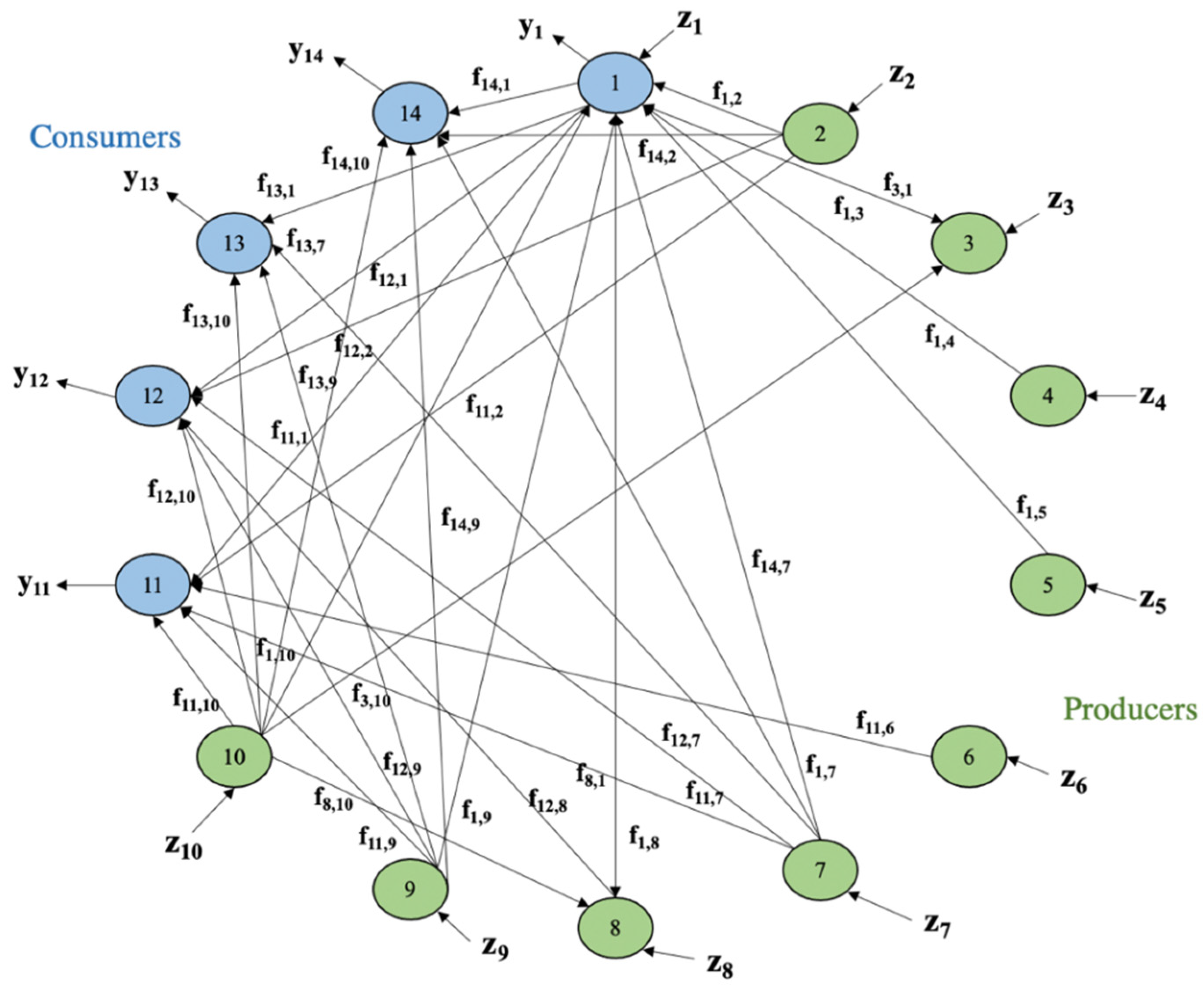
Altogether, the U.S. energy system is modeled here as a system comprised of 14 compartments that form a complex network of direct and indirect energy flows (reject energy, energy services, and electricity imports are considered outputs and input). This analysis will take the direct flows as input, and the indirect flows will be calculated as output. Now that we have defined the compartments that exchange energy between each other, we have completed one step of setting up an ENA. We have defined the actors within the U.S. energy industry, but we must establish system boundaries. Data used to quantify direct flows mainly came from the U.S. Energy Information Administration (EIA). Energy flow diagrams from the Lawrence Livermore National Laboratory (LLNL) were used to quantify direct flows and help visualize where specific types of energy go; LLNL derived their energy flow diagrams from EIA and DOE sources [16,17,18]. An example of the LLNL’s energy flow diagrams is shown below for 2019 in Figure 2.

The next step to setting up an ENA is defining system boundaries. The state lines bordering Pennsylvania, West Virginia, Virginia, Delaware, and the District of Columbia that define the state of Maryland define the system’s boundary. Energy flows entering state lines and terminating inside are viewed as input, and flows exiting state lines beginning inside are viewed as output (including flows that exist in the atmosphere through dissipation). All other flows between compartments inside state lines are valid flows, as are inputs and outputs. Flows that begin and terminate outside of state lines do not exist within system boundaries and are, therefore, not included in the analysis. Finally, the last step is to define an energy currency, meaning the units or type of energy flow between compartments. The energy currency for this study will be presented in British thermal units (Btu), as the standard unit of energy currency in the USA, as well as SI units (kilojoules). Though different types of energy producers are the highlight of this analysis, the focus is on the proportions of the energy they produce and where these proportions go. Each type of energy was converted to its Btu equivalent to adhere to one energy currency that’s required by ENA. Therefore, the focus of this study is to examine the proportion of contributions from each type of energy producer relative to all others. The goal is to identify patterns or trends related to specific types of energy within the Maryland energy industry and evaluate how they affect the network holistically. ENA provides useful indicators that quantitatively describe a system’s state. They will be used in this paper’s analysis.

The energy flowing out of a compartment must be equal to the energy flowing into that compartment to obey the conservation of energy; inflows and outflows include imports, exports, and intercompartmental flows. For this study’s purposes, compartments are treated as having no storage in this analysis. Instances where energy may be temporarily stored prior to production and consumption, do not impact the Maryland energy system’s flows because of the flows’ magnitudes. In other words, compartment storages are negligible in this analysis. Because each compartment must obey the conservation of matter, the row and column for each compartment must sum to the same value, meaning the sum of inputs to a compartment must equal the sum of outputs from that compartment. Consequently, each direct flow matrix will be balanced. Only balanced flow matrices can be used in ENA because they reflect steady-state or quasi-steady state systems. Unbalanced flow matrices represent systems that are in a dynamic and non-steady state and cannot be used in ENA.

The Maryland energy system’s inputs can be represented by

$$T^{in}=z_i+{\displaystyle \sum }_{j=1}{f}_{ji}$$

(1)

where $z_i$ represents flow inputs to compartment, i and $f_{ji}$ represent intercompartmental flows from compartment j to compartment i; note that $f_{ji}$ represents flows from j to i is convention in ENA. $T^{in}$ is then the total inflows to compartment i. The equation below represents the outflows from compartment i.

$$T^{out}=y_i+{\displaystyle \sum }_{j=1}{f}_{ji}$$

(2)

where $y_i$ represents flow outputs from compartment i. The two above equations can be equated to each other knowing that each compartment must obey the conservation of energy.

$$T^{out}=T^{in}$$

(3)

Because this study applies ENA to an industrial system, compartments will inevitably have energy losses. The losses from individual compartments are not considered—all losses are assigned to the electricity sector. A useful quantity that is the basis for flow-based metrics is the total system throughflow (TST). TST is the sum of all compartment’s inflows or outflows (inflow and outflow sums should be equal according to the steady-state requirement necessary for ENA).

$$TST={\displaystyle \sum }_{i=1}{T}_i^{in}={\displaystyle \sum }_{i=1}{T}_i^{out}$$

(4)

A system’s TST represents the amount of energy being used within that system and can be an indicator of its growth and development. With compartmental throughflows and total system throughflow defined, we can define the dimensionless flow intensity matrix G, whose matrix elements are $g_{ij}=\frac{f_{ij}}{T_j}$. The flow intensity matrix represents each flow going into a compartment as a fraction of that compartment’s total throughflow. In other words, the G matrix represents each flow as an intensity relative to the total throughflow. By raising the G matrix to powers of m, one is determining the flow intensities corresponding to flows that travel n path lengths before terminating. Indirect flows will be revealed when considering m values greater than two. The elements of the G matrix approach zero as the order n approaches infinity, which defines a new matrix called the integral flow matrix N.

$$\mathrm{N}=\left[{\mathrm{n}}_{ij}\right]={\displaystyle \sum }_{\mathrm{m}=0}^{\infty }{\mathrm{G}}^{\mathrm{m}}={\left(\mathrm{I}-\mathrm{G}\right)}^{-1}$$

(5)

The cycled flows in a system can be derived from the integral flow matrix as follows

$$CF={\displaystyle \sum }_{\mathrm{j}=1}\frac{{\mathrm{n}}_{\mathrm{jj}}-1}{{\mathrm{n}}_{\mathrm{jj}}}{\mathrm{T}}_{\mathrm{j}}$$

(6)

Cycled flows come from G matrix elements of order m = 2 or greater. Finally, a quantity called the Finn cycling index (FCI) that’s used to quantify the amount of cycling present in a system relative to total system throughflow is calculated using the cycled flows.

$$\mathrm{FCI}=\frac{CF}{TST}$$

(7)

Altogether, total system throughflow is a measure of the total amount of energy a system is using. It is used as a relative standard to compare all other types of flows and related indicators, such as cycled flows and the Finn cycling index. Cycled flows represent flows that return to a compartment before it leaves the system’s boundaries. Systems with many cycled flows relative to their total system throughflow will display high cycling indices and represent increasingly sustainable systems because system actors are using recycled energy. Cycled flows are, therefore, an indicator of a system’s efficiency. If actors within a system are reusing energy flows, less TST is necessary to sustain the system, making the system efficient in its energy usage.

The ENA indicators used to analyze Maryland’s energy industry in this study are TST, boundary flows, first pass flows, cycled flows, Finn cycling index, and indirectness. Indirectness is an indicator used to quantify what’s commonly referred to as the dominance of indirect effects, which measures the contributions of a system’s indirect flows to its direct flows. This indicator is calculated by taking the ratio of indirect flows to indirect flows as follows

$$Indirect/Direct=\frac{{{\displaystyle \sum }}_{i, j=1}^n\left(n_{ij}-g_{ij}-{\mathrm{i}}_{ij}\right)}{{{\displaystyle \sum }}_{i,j=1}^n{g}_{ij}}$$

(8)

where $n_{ij}$ represents the integral flow matrix elements and ${\mathrm{i}}_{ij}$ represents the identity matrix.

Generally, ecological systems display indirectness ratios greater than one, which speaks to the great interconnectedness of natural ecosystems—actors receive more energy or material contributions that have passed through one or more actors rather than energy or material coming directly from one actor or boundary inflows. However, as this study shows, industrial ecosystems such as the energy industry exhibit less indirectness. In other words, there is no dominance of indirect flows, and actors receive energy primarily from one actor or boundary inflows which explain the inefficiency of human-made energy systems relative to natural ecosystems.

MATLAB was used to carry out the ENA for this study. A MATLAB function, “NEA.m,” developed by Brian Fath and Stuart Borrett, takes the input of intercompartmental flows, compartmental storages, and boundary input and output flows and outputs ENA properties; the ENA properties used in this study are the TST, boundary flows, first pass flows, cycled flows, Finn cycling index, and indirectness [23]. Compartmental storages refer to a system compartment’s energy or material storage capacity, which is not translatable to the industrial ecosystem that is Maryland’s energy industry. Because of this, the compartmental storages for all actors in this study were taken to be represented by a column vector of ones in the flow matrices.

Maryland’s RPS sets goals for the contributions of renewable energy sources to electricity generation. In other words, the RPS does not quantify renewables’ contributions to the end-use sectors within the Maryland energy system. First, rough linear trends were applied to the contributions of each energy producer to the electricity sector over the years 2010–2019; contributions to end-use sectors were kept at 2019 flow values. These trends were used to estimate energy producers’ (other than solar and wind energy since their contributions were set by the RPS) flow values in the year 2030. Petroleum was the only energy source with modified 2030 flow values for end-use sectors; averages of petroleum flow for all energy acceptors were calculated from 2010–2019 and applied to their 2030 flow matrix. Second, the ratios of each energy producer’s flow to the electricity sector to the electricity sector’s total throughflow in 2019 were calculated. Third, all flows to the electricity sector were summed in the new 2030 flow matrix, and the difference between that and the 2019 electricity sector total throughflow was calculated. The ratios were then applied to the difference in electricity sector throughflows, and these flows represented additions to the 2030 electricity sector. Coal was erased from the flow matrix following its sharp decline from 2010–2019 and according to efforts attempting to eliminate coal use in Maryland (although it remains a coal-producing state) [24].

Finally, the flow data for renewables’ contribution to electricity generation were calculated. Wind energy’s 2022.5 MW_e was converted to its trillion Btu equivalent and added to its 2019 electricity sector flow value. This addition to wind energy’s capacity set by the RPS turned out to be insignificant given the ultimate goal of 50% renewable electricity generation; wind energy was required to add much more electricity-generating capacity to meet this goal. Solar’s 2019 energy flow to the electricity generation was increased until it reached 14.5% of electricity generation. Finally, biomass was increased to support solar and wind energy’s increased electricity generation demand set by the RPS; biomass is considered a renewable energy source according to Maryland’s RPS.

3. Results and Discussion

Total system throughflow generally decreased from 2010 to 2019 with some fluctuation in 2018, meaning overall Maryland decreased its total energy usage over the nine-year span. Figure 3 depicts Maryland’s TST. Red dots correspond to data points; blue lines serve simply to connect data points. This graphical convention will be used for all figures that follow.

A massive reduction in coal use is responsible for the decrease in TST. Coal usage over 2010–2019 was at its highest in 2010 with the use of 270 trillion Btu (2.85 × 10¹⁴ kJ) for electricity generation and industrial and commercial purposes. In 2019 coal usage reached its lowest usage in the energy industry, with only 77.3 trillion Btu (8.16 × 10¹³ kJ) used for electricity generation and industrial purposes. A small increase in TST breaks the steady downward trend in 2014, which is due to an uptick in coal usage and an abnormal increase in nuclear usage; nuclear energy production generally remains at 150 trillion Btu (1.58 × 10¹⁴ kJ) annually because all nuclear energy is produced at one Maryland facility. The most notable break in the general downward trend in Maryland’s TST is in 2018. The summers of 2018 and 2019 had record-setting temperatures. The summer of 2018 was ranked the fourth hottest in the U.S., and the summer of 2019 became the hottest ever experienced in the northern hemisphere [25,26]. These record-setting temperatures likely contributed to above-average electricity consumption to cool buildings and homes. LLNL flow diagrams for the U.S. during the years 2018 and 2019 reinforce these hot summers [16]. Between 2010 and 2017, the average national energy consumption was 97.3 quadrillion Btu (1.02 × 10¹⁷ kJ). In 2018 and 2019, the national energy consumption reached 101.2 and 100.2 quadrillion Btu (1.067 × 10¹⁸ and 1.057 × 10¹⁸ kJ), respectively, indicating the overall climate exhibited temperature anomalies during those years. On a more local scale, TST increased in 2018 and 2019 in Maryland due to another increase in coal usage and a large increase in natural gas usage. Natural gas increased from 233–313 trillion Btu (2.46 − 3.30 × 10¹⁴ kJ) between 2018 and 2019. Coal usage increased from 107–124 trillion Btu (1.13 − 1.31 × 10¹⁴ kJ) between 2018 and 2019, which is still notably smaller than its usage in 2010, hinting at the general effort to reduce coal usage in Maryland energy production. Ultimately, reducing total energy usage while maintaining current cycling levels will benefit the cyclability of the energy industry. This is based on equation 7, which indicates the relation between the two measures. Therefore, a TST-centric approach to creating a leaner and more efficient energy industry would be to reduce total energy usage when possible [13]. This approach will be challenging, as the 2030 simulation will show, because there seems to be a balance between a diverse energy industry (i.e., renewables and non-renewables) and a clean energy industry (i.e., almost only renewables) that must be met to create a system with high cyclability.

Boundary and first pass flows represent energy coming into or exiting system boundaries and flows that pass through a compartment for the first time, respectively. Figure 4 shows both flow types.

Boundary and first pass flows exactly mimic TST and, when combined, make up 99.99% of the TST every year from 2010–2019. This shows that cycled flows are practically negligible, meaning energy flows are generally used by compartments once, and energy is either passed to another compartment or expelled from the system.

The system’s linearity is not surprising. Natural ecosystems typically contain more actors than human-made industrial ecosystems (depending on how one defines an industrial system’s actors), and they certainly have more pathways for energy to flow. The additional pathways found in natural ecosystems are primarily responsible for their high cyclability and energy use efficiency. Compared to industrial ecosystems, nature has established much more efficient and synergistic energy systems [4,5,11]. Figure 5 shows the cycled flows for Maryland’s energy industry.

The cycled flows from 2010–2019 seem to be sporadic. Despite consistent fluctuations, cycled flows range from 0.185 and 0.193 trillion Btu (1.95 − 2.04 × 10¹¹ kJ), which is practically insignificant in comparison to the magnitude of TST, boundary, and first pass flows. The insignificance of cycled flows is magnified when examining the energy industry’s Finn cycling indices from 2010–2019 in Figure 6.

Figure 6 is the inverse of Figure 3. Looking at equation 7 again, cycled flows are essentially a constant, and TST is the only variable, which corroborates the fact that the fluctuating behavior of cycled flows is negligible. Thus, the fact that the time-dependent cycling index is the exact inverse of the time-dependent TST, further verifying that Maryland’s energy industry exhibits very little cycling.

The measure of indirectness for the energy industry proved to be interesting. The system’s indirectness increased steadily from 2010–2019, with a small fluctuation in 2018. Figure 7 shows the system’s indirectness.

This measure calculated indirectness by normalizing output flows. Renewable energy sources generally feed the electricity sector for distribution to end-use sectors, adding indirect paths to the system’s energy flows. During 2010–2019, renewable energy sources increased. Solar and wind energy generally increased from 2010–2019 to achieve RPS goals. Because the energy produced by renewables increased during this time frame, indirect paths were added to the system, increasing the indirectness. Thus, increasing the usage of renewables adds indirect paths and, thereby, cyclability to a system. This is reinforced by the increase in the cycling index found in the 2030 simulation results.

Maryland’s 2030 RPS Simulation

Maryland’s RPS goal of 50% renewable electricity generation appears to be an ambitious undertaking. Wind energy’s total throughflow exceeded its mandated addition of 2022.5 MW_e to wind infrastructure by a factor of 2.4. The mandate for solar to contribute to 14.5% of electricity generation also added significantly to the TST for interconnected reasons.

Table 3. Electricity generation by energy source simulated for year 2030.

	Solar	Nuclear	Hydro	Wind	Geothermal	Natural Gas	Coal	Biomass	Petroleum
2019	1.2%	43.6%	5.4%	1.3%	0%	27.8%	18.6%	1.9%	0.2%
2030	14.8%	17.9%	2.2%	16.5%	0%	31.8%	0%	16.5%	0.3%

compares 2019 and 2030 for the percentage of each energy source’s contribution to electricity generation.

Table 4. Direct flow matrix for Maryland’s simulated RPS for year 2030. Ele = electricity; sol = solar; nuc = nuclear; hyd = hydro; geo = geothermal; NG = natural gas; bio = biomass; pet = petroleum; res = residential; ind = industrial; tra = transportation; com = commericial; in = input; st = storage; out = output.

	Ele.	Sol.	Nuc.	Hyd.	Wind	Geo.	NG	Bio.	Pet.	Res.	Ind.	Tra.	Com.	In.	St.
Ele.	0	130	157	19.5	145	0	279	145	2.65	0	0	0	0	85.6	1
Sol.	0	0	0	0	0	0	0	0	0	0	0	0	0	138.92	1
Nuc.	0.29	0	0	0	0	0	0	0	1.34	0	0	0	0	157	1
Hyd.	0	0	0	0	0	0	0	0	0	0	0	0	0	19.5	1
Wind	0	0	0	0	0	0	0	0	0	0	0	0	0	145	1
Geo.	0	0	0	0	0	0	0	0	0	0	0	0	0	0.57	1
NG	0	0	0	0	0	0	0	0	0	0	0	0	0	471.06	1
Bio.	0	0	0	0	0	0	0	0	0	0	0	0	0	179.3	1
Pet.	0	0	0	0	0	0	0	0	0	0	0	0	0	436.94	1
Res.	202.9	6.1	0	0	0	0.57	85.6	5.5	22.3	0	0	0	0	0	1
Ind.	27.4	0.32	0	0	0	0	19.2	4	1.84	0	0	0	0	0	1
Tra.	4.3	0	0	0	0	0	7.46	22.4	393.4	0	0	0	0	0	1
Com.	213.1	2.5	0	0	0	0	79.8	2.4	15.37	0	0	0	0	0	1
Out.	516.45	0	0	0	0	0	0	0	0	322.98	52.81	427.58	313.13	0	1

shows the direct flow matrix for the year 2030. See Appendix A (

Table A1. Direct flow matrices used as ENA input. Nomenclature: ele = electricity; sol = solar; nuc = nuclear; hyd = hydro; geo = geothermal; NG = natural gas; bio = biomass; pet = petroleum; res = residential; ind = industrial; tra = transportation; com = commericial; in = input; st = storage; out = output. Nomenclature are necessary to make the flow matrices legible. The year above each flow matrix corresponds to the energy data pertinent to Maryland’s energy industry in the labeled year.

(a) 2010
	Ele.	Sol.	Nuc.	Hyd.	Wind	Geo.	NG	Coal	Bio.	Pet.	Res.	Ind.	Tra.	Com.	In.	St.
Ele.	0	0.01	150	16	0.015	0	32	240	7.6	3.9	0	0	0	0	87	1
Sol.	0	0	0	0	0	0	0	0	0	0	0	0	0	0	0.21	1
Nuc.	0.13	0	0	0	0	0	0	0	0	1.34	0	0	0	0	150	1
Hyd.	0	0	0	0	0	0	0	0	0	0	0	0	0	0	16	1
Wind	0	0	0	0	0	0	0	0	0	0	0	0	0	0	0.015	1
Geo.	0	0	0	0	0	0	0	0	0	0	0	0	0	0	0.55	1
NG	0	0	0	0	0	0	0	0	0	0	0	0	0	0	220	1
Coal	0.02	0	0	0	0	0	0	0	0	0.06	0	0	0	0	270	1
Bio.	0	0	0	0	0	0	0	0	0	0	0	0	0	0	48	1
Pet.	0	0	0	0	0	0	0	0	0	0	0	0	0	0	500	1
Res.	99	0.2	0	0	0	0.55	86	0	8.7	29	0	0	0	0	0	1
Ind.	17	0	0	0	0	0	24	23	9.1	36	0	0	0	0	0	1
Tra.	1.9	0	0	0	0	0	6.7	0	19	420	0	0	0	0	0	1
Com.	100	0	0	0	0	0	69	0.47	3.4	12	0	0	0	0	0	1
Out.	310	0	0	0	0	0	0	0	0	0	218	109	444	187	0	1
(b) 2011
	Ele.	Sol.	Nuc.	Hyd.	Wind	Geo.	NG	Coal	Bio.	Pet.	Res.	Ind.	Tra.	Com.	In.	St.
Ele.	0	0.026	150	25	2.6	0	22	220	7	2.8	0	0	0	0	86	1
Sol.	0	0	0	0	0	0	0	0	0	0	0	0	0	0	0.3	1
Nuc.	0.13	0	0	0	0	0	0	0	0	1.34	0	0	0	0	150	1
Hyd.	0	0	0	0	0	0	0	0	0	0	0	0	0	0	25	1
Wind	0	0	0	0	0	0	0	0	0	0	0	0	0	0	2.6	1
Geo.	0	0	0	0	0	0	0	0	0	0	0	0	0	0	0.53	1
NG	0	0	0	0	0	0	0	0	0	0	0	0	0	0	200	1
Coal	0.02	0	0	0	0	0	0	0	0	0.06	0	0	0	0	240	1
Bio.	0	0	0	0	0	0	0	0	0	0	0	0	0	0	48	1
Pet.	0	0	0	0	0	0	0	0	0	0	0	0	0	0	480	1
Res.	93	0.28	0	0	0	0.53	80	0	8.9	24	0	0	0	0	0	1
Ind.	17	0	0	0	0	0	22	22	9.5	37	0	0	0	0	0	1
Tra.	1.9	0	0	0	0	0	6.4	0	20	400	0	0	0	0	0	1
Com.	100	0	0	0	0	0	69	0.62	3.6	12	0	0	0	0	0	1
Out.	300	0	0	0	0	0	0	0	0	0	202	107	430	187	0	1
(c) 2012
	Ele.	Sol.	Nuc.	Hyd.	Wind	Geo.	NG	Coal	Bio.	Pet.	Res.	Ind.	Tra.	Com.	In.	St.
Ele.	0	0.2	140	16	3.1	0	51	170	7.4	1.5	0	0	0	0	91	1
Sol.	0	0	0	0	0	0	0	0	0	0	0	0	0	0	2	1
Nuc.	0.13	0	0	0	0	0	0	0	0	1.34	0	0	0	0	140	1
Hyd.	0	0	0	0	0	0	0	0	0	0	0	0	0	0	16	1
Wind	0	0	0	0	0	0	0	0	0	0	0	0	0	0	3.1	1
Geo.	0	0	0	0	0	0	0	0	0	0	0	0	0	0	0.57	1
NG	0	0	0	0	0	0	0	0	0	0	0	0	0	0	220	1
Coal	0.01	0	0	0	0	0	0	0	0	0.05	0	0	0	0	190	1
Bio.	0	0	0	0	0	0	0	0	0	0	0	0	0	0	49	1
Pet.	0	0	0	0	0	0	0	0	0	0	0	0	0	0	470	1
Res.	91	1.8	0	0	0	0.57	73	0	8.3	19	0	0	0	0	0	1
Ind.	15	0	0	0	0	0	18	20	9.6	34	0	0	0	0	0	1
Tra.	1.8	0	0	0	0	0	7.9	0	20	400	0	0	0	0	0	1
Com.	100	0	0	0	0	0	67	0.61	3.7	11	0	0	0	0	0	1
Out.	270	0	0	0	0	0	0	0	0	0	198	98	430	185	0	1
(d) 2014
	Ele.	Sol.	Nuc.	Hyd.	Wind	Geo.	NG	Coal	Bio.	Pet.	Res.	Ind.	Tra.	Com.	In.	St.
Ele.	0	0.9	150	15.4	3.1	0	51	185.4	7.9	5.3	0	0	0	0	90.7	1
Sol.	0	0	0	0	0	0	0	0	0	0	0	0	0	0	4.3	1
Nuc.	0.13	0	0	0	0	0	0	0	0	1.34	0	0	0	0	150	1
Hyd.	0	0	0	0	0	0	0	0	0	0	0	0	0	0	15.4	1
Wind	0	0	0	0	0	0	0	0	0	0	0	0	0	0	3.1	1
Geo.	0	0	0	0	0	0	0	0	0	0	0	0	0	0	0.57	1
NG	0	0	0	0	0	0	0	0	0	0	0	0	0	0	217	1
Coal	0.01	0	0	0	0	0	0	0	0	0.05	0	0	0	0	201	1
Bio.	0	0	0	0	0	0	0	0	0	0	0	0	0	0	53.8	1
Pet.	0	0	0	0	0	0	0	0	0	0	0	0	0	0	461	1
Res.	93.8	3.4	0	0	0	0.57	95.1	0	11.5	26.8	0	0	0	0	0	1
Ind.	13.1	0	0	0	0	0	15.5	15.5	8.5	33	0	0	0	0	0	1
Tra.	1.9	0	0	0	0	0	6.9	0	23	384	0	0	0	0	0	1
Com.	102	0.03	0	0	0	0	78.6	0.1	3	12.1	0	0	0	0	0	1
Out.	269	0	0	0	0	0	0	0	0	0	230.8	85.6	415.3	195.4	0	1
(e) 2015
	Ele.	Sol.	Nuc.	Hyd.	Wind	Geo.	NG	Coal	Bio.	Pet.	Res.	Ind.	Tra.	Com.	In.	St.
Ele.	0	1	153	15.1	4.1	0	41.8	151	7.8	2.7	0	0	0	0	94.5	1
Sol.	0	0	0	0	0	0	0	0	0	0	0	0	0	0	4.4	1
Nuc.	0.13	0	0	0	0	0	0	0	0	1.34	0	0	0	0	153	1
Hyd.	0	0	0	0	0	0	0	0	0	0	0	0	0	0	15.1	1
Wind	0	0	0	0	0	0	0	0	0	0	0	0	0	0	4.1	1
Geo.	0	0	0	0	0	0	0	0	0	0	0	0	0	0	0.57	1
NG	0	0	0	0	0	0	0	0	0	0	0	0	0	0	227	1
Coal	0.01	0	0	0	0	0	0	0	0	0.05	0	0	0	0	166	1
Bio.	0	0	0	0	0	0	0	0	0	0	0	0	0	0	47.6	1
Pet.	0	0	0	0	0	0	0	0	0	0	0	0	0	0	474	1
Res.	93.5	1.4	0	0	0	0.57	87.5	0	5.8	27.2	0	0	0	0	0	1
Ind.	13.3	0.12	0	0	0	0	15.6	15	7.9	31.8	0	0	0	0	0	1
Tra.	1.8	0	0	0	0	0	7.8	0	23.3	392	0	0	0	0	0	1
Com.	102	1.8	0	0	0	0	74.1	0.01	2.9	19.4	0	0	0	0	0	1
Out.	260	0	0	0	0	0	0	0	0	0	215.5	83.7	425.3	200	0	1
(f) 2016
	Ele.	Sol.	Nuc.	Hyd.	Wind	Geo.	NG	Coal	Bio.	Pet.	Res.	Ind.	Tra.	Com.	In.	St.
Ele.	0	1.9	154	12.9	4.9	0	52	151	7.6	2.1	0	0	0	0	94.5	1
Sol.	0	0	0	0	0	0	0	0	0	0	0	0	0	0	4.4	1
Nuc.	0.13	0	0	0	0	0	0	0	0	1.34	0	0	0	0	153	1
Hyd.	0	0	0	0	0	0	0	0	0	0	0	0	0	0	15.1	1
Wind	0	0	0	0	0	0	0	0	0	0	0	0	0	0	4.1	1
Geo.	0	0	0	0	0	0	0	0	0	0	0	0	0	0	0.57	1
NG	0	0	0	0	0	0	0	0	0	0	0	0	0	0	227	1
Coal	0.01	0	0	0	0	0	0	0	0	0.04	0	0	0	0	166	1
Bio.	0	0	0	0	0	0	0	0	0	0	0	0	0	0	47.6	1
Pet.	0	0	0	0	0	0	0	0	0	0	0	0	0	0	474	1
Res.	93.2	3	0	0	0	0.57	79.9	0	4.8	18.2	0	0	0	0	0	1
Ind.	13	0.32	0	0	0	0	16.2	12.1	8.7	30.6	0	0	0	0	0	1
Tra.	1.8	0	0	0	0	0	8	0	22.4	380	0	0	0	0	0	1
Com.	101	1.7	0	0	0	0	74.1	0	2.9	16.9	0	0	0	0	0	1
Out.	267	0	0	0	0	0	0	0	0	0	199.8	81	412.6	196.8	0	1
(g) 2017
	Ele.	Sol.	Nuc.	Hyd.	Wind	Geo.	NG	Coal	Bio.	Pet.	Res.	Ind.	Tra.	Com.	In.	St.
Ele.	0	2.4	158	18.1	5.2	0	53.1	94.7	7.8	1.4	0	0	0	0	94.2	1
Sol.	0	0	0	0	0	0	0	0	0	0	0	0	0	0	9.3	1
Nuc.	0.13	0	0	0	0	0	0	0	0	1.34	0	0	0	0	158	1
Hyd.	0	0	0	0	0	0	0	0	0	0	0	0	0	0	18.1	1
Wind	0	0	0	0	0	0	0	0	0	0	0	0	0	0	5.2	1
Geo.	0	0	0	0	0	0	0	0	0	0	0	0	0	0	0.57	1
NG	0	0	0	0	0	0	0	0	0	0	0	0	0	0	233	1
Coal	0.01	0	0	0	0	0	0	0	0	0.05	0	0	0	0	107	1
Bio.	0	0	0	0	0	0	0	0	0	0	0	0	0	0	45.4	1
Pet.	0	0	0	0	0	0	0	0	0	0	0	0	0	0	442	1
Res.	89	4.7	0	0	0	0.57	79.4	0	4.8	16.9	0	0	0	0	0	1
Ind.	13	0.31	0	0	0	0	16.5	12.3	8.1	30.6	0	0	0	0	0	1
Tra.	1.8	0	0	0	0	0	8.5	0	22.3	376	0	0	0	0	0	1
Com.	98.6	1.9	0	0	0	0	75.7	0	2.4	16.8	0	0	0	0	0	1
Out.	232	0	0	0	0	0	0	0	0	0	195.3	80.6	408.9	195.3	0	1
(h) 2018
	Ele.	Sol.	Nuc.	Hyd.	Wind	Geo.	NG	Coal	Bio.	Pet.	Res.	Ind.	Tra.	Com.	In.	St.
Ele.	0	3.5	157	25.8	5.2	0	101	112	7.7	3.2	0	0	0	0	75.1	1
Sol.	0	0	0	0	0	0	0	0	0	0	0	0	0	0	11.5	1
Nuc.	0.13	0	0	0	0	0	0	0	0	1.34	0	0	0	0	157	1
Hyd.	0	0	0	0	0	0	0	0	0	0	0	0	0	0	25.8	1
Wind	0	0	0	0	0	0	0	0	0	0	0	0	0	0	5.2	1
Geo.	0	0	0	0	0	0	0	0	0	0	0	0	0	0	0.57	1
NG	0	0	0	0	0	0	0	0	0	0	0	0	0	0	313	1
Coal	0.01	0	0	0	0	0	0	0	0	0.04	0	0	0	0	124	1
Bio.	0	0	0	0	0	0	0	0	0	0	0	0	0	0	46	1
Pet.	0	0	0	0	0	0	0	0	0	0	0	0	0	0	449	1
Res.	96	5.4	0	0	0	0.57	90.2	0	5.8	21.8	0	0	0	0	0	1
Ind.	13.2	0.34	0	0	0	0	16.9	11.9	7.7	26.9	0	0	0	0	0	1
Tra.	1.8	0	0	0	0	0	24.3	0	22.2	380	0	0	0	0	0	1
Com.	101	2.2	0	0	0	0	80.7	0	2.6	18.4	0	0	0	0	0	1
Out.	279	0	0	0	0	0	0	0	0	0	219.9	76.9	427.9	204.6	0	1
(i) 2019
	Ele.	Sol.	Nuc.	Hyd.	Wind	Geo.	NG	Coal	Bio.	Pet.	Res.	Ind.	Tra.	Com.	In.	St.
Ele.	0	4.2	157	19.5	4.6	0	100	67.1	6.7	1	0	0	0	0	85.6	1
Sol.	0	0	0	0	0	0	0	0	0	0	0	0	0	0	13.1	1
Nuc.	0.13	0	0	0	0	0	0	0	0	1.34	0	0	0	0	157	1
Hyd.	0	0	0	0	0	0	0	0	0	0	0	0	0	0	19.5	1
Wind	0	0	0	0	0	0	0	0	0	0	0	0	0	0	4.6	1
Geo.	0	0	0	0	0	0	0	0	0	0	0	0	0	0	0.57	1
NG	0	0	0	0	0	0	0	0	0	0	0	0	0	0	311	1
Coal	0.01	0	0	0	0	0	0	0	0	0.04	0	0	0	0	77.3	1
Bio.	0	0	0	0	0	0	0	0	0	0	0	0	0	0	41	1
Pet.	0	0	0	0	0	0	0	0	0	0	0	0	0	0	474	1
Res.	93.9	6.1	0	0	0	0.57	85.6	0	5.5	17.6	0	0	0	0	0	1
Ind.	12.7	0.32	0	0	0	0	19.2	10.2	4	27.8	0	0	0	0	0	1
Tra.	2	0	0	0	0	0	26.5	0	22.4	409	0	0	0	0	0	1
Com.	98.6	2.5	0	0	0	0	79.8	0	2.4	19.8	0	0	0	0	0	1
Out.	239	0	0	0	0	0	0	0	0	0	209.3	74.1	459.5	203	0	1

Inputs represent the inherent amount of energy each energy producer has (this includes electricity imports). Outputs represent energy services and reject energy. The storage vector required to run the NEA.m program was assigned as a column vector of ones. The actors in this energy system do not have associated energy that is inherent to them.

) for comparison with 2010–2019 direct flow matrices.

Coal was entirely removed from the energy industry, which initially comprised a considerable portion of the total energy provided by energy producers. This absence of coal energy required biomass, renewable energy by RPS standards, and natural gas, a cleaner but non-renewable energy, to support the main renewable energies: solar and wind. It would be impractical only to increase solar and wind energies for two reasons. First, relying solely on solar and wind energy as renewable energy in the future would create a much less diverse energy industry which theoretically would not benefit the energy system holistically. Removing energy sources or reducing the energy capacity of energy sources translates to removing or restricting energy flow pathways. Second, if solar and wind energy were to take on most of the renewable energy generation, this would require a significant increase in solar and wind infrastructure, given its current status. The total throughflow for solar and wind energies increased by factors of about 10 and 30, respectively, from 2019 to 2030. These factors would increase even more if biomass and natural gas did not increase as well. Figure 8 shows the TST for the year 2030 in comparison to 2010–2019 TST data.

The TST increased from 2491 trillion Btu (2.63 × 10¹⁵ kJ) in 2019 to 3630 trillion Btu (3.83 × 10¹⁵ kJ) in 2030, indicating the total energy demand will continue to increase during the coming years. The vast increase in TST originates with the need for immense growth in the two primary renewables that the RPS sets quantified goals for Solar and wind. Solar and wind in 2019 contributed 13.1 and 4.6 trillion Btu (1.38 × 10¹³ kJ and 4.85 × 10¹² kJ), respectively, to the electricity sector. To reach solar and wind goals set by Maryland’s RPS, solar and wind electricity sector contributions increased to 130 and 145 trillion Btu (1.37 − 1.53 × 10¹⁴ kJ), respectively. These values were balanced among each other by choice to produce a more distributed and balanced energy system theoretically; other renewable and clean energy sources could have been reduced to make solar energy’s production lesser, but these reductions would be unrealistic and not follow the 2010–2019 energy trends. In addition to solar and wind energy, biomass and natural gas significantly increased to support RPS goals. From 2019 to 2030, biomass increased from 41 to 179 trillion Btu (4.32 × 10¹³ to 1.89 × 10¹⁴ kJ), and natural gas increased from 311 to 471 trillion Btu (3.28 − 4.97 × 10¹⁴ kJ). Biomass consumption has never surpassed 53.8 trillion Btu (5.68 × 10¹³ kJ) between 2010 and 2019, indicating that a yearly consumption of 179 trillion Btu is unrealistic. Waste-to-energy energy facilities would have to process more than three times more waste than usual, making an increase to 179 trillion Btu unrealistic. Thus, four renewable/clean energy sources saw large total throughflow growth between 2019 and 2030, resulting in the vast increase in Maryland’s TST evident in Figure 8. Petroleum consumption from 2019 to 2030 decreased mildly from 476 to 436 trillion Btu (over a decrease of 4.22 × 10¹³ kJ). With coal being the only other fossil fuel source that decreased (77 to 0 trillion Btu), the TST in 2030 increased overall. Another approach would be to focus more heavily on energy efficiency and demand reduction strategies that could actually decrease TST or at least decrease the rate of increase, beginning to flatten the curve.

As expected, the boundary and first pass flows closely mimic the TST behavior when simulating 2030. Figure 9 includes the 2030 boundary and first pass flows.

Boundary and first pass flows in 2030 comprise 99.99% of TST, exhibiting the same behavior as in the years 2010–2019. This implies that Maryland’s energy industry remains linear despite achieving RPS goals. The goal of renewable energy standards is reached through supply-side approaches, not focusing on synergies of a circular economy or reduced demand.

There is an increased ratio of the first pass to boundary flows from 2019 to 2030. This may be because more renewables will be implemented at the utility-scale in the future, which will add more paths from renewables to end-users. Utility-scale renewables will feed the electricity sector for distribution more often than today’s energy infrastructure, which relies heavily on direct energy consumption by end-users via rooftop solar panels, for example.

The cycled flows in 2030 reached 0.33 trillion Btu (3.48 × 10¹¹ kJ), an increase of 0.14 trillion Btu from 2019. The cycling index for 2030 disrupted the inverse relationship between TST and cycling index, that is evident in Figure 3 and Figure 6. The year 2030 experiences the largest cycling index, likely because renewables usage has increased. Renewable energy sources are typically fed into the electricity sector for distribution to end-users, unlike non-renewable sources such as petroleum. This extra step before energy distribution for renewables creates an extra flow pathway which could lead to more cycled flows and thus higher cycling indices. Therefore, with more renewable energy sources, Maryland’s energy industry can expect to see higher cycling indices.

Figure 10 displays the cycling indices from 2010–2019, including 2030. Because cyclability is associated with a system’s ability to use energy or materials efficiently, this result indicates that increasing renewable energy usage may result in more efficient energy systems. Producing energy through renewable means, such as solar panels and wind turbines, typically requires a mediator to convert or redistribute that energy to end users. This opens additional energy flow pathways, thereby increasing the potential for more interconnectedness. Therefore, an energy industry’s ability to use energy efficiently relates to how the system is structured. Energy flows between compartments depend on the available pathways in a system, and Maryland’s simulated 2030 energy system has 29 available pathways for 14 actors. Increasing the number of pathways for energy to flow would increase the cyclability of the energy industry. This would entail distributing more energy sources to more energy consumers, like building wind energy infrastructure so that all end-use sectors can receive wind-derived energy.

The indirectness indicator for the 2030 simulation is surprising. By increasing renewable energy usage, it was expected that indirect paths would increase and, therefore, indirectness would increase. This is because renewable energy sources typically feed the electricity sector for distribution to end-use sectors, thereby increasing indirect energy flows. Despite increasing renewable energy sources to reach 50% renewable electricity generation, the indirectness for Maryland’s energy industry stayed the same. Figure 11 shows the indirectness for 2030.

Further analysis into the flow intensity (G) and integral flow (N) matrices by compartment may reveal reasons for the unexpectedly low indirectness value of 2030. Identified reasons could potentially reveal insights into how to optimize indirect paths within Maryland’s energy industry and subsequently increase cycling. ENA, by nature, combines the direct and indirect effects in its indicators. Thus, the indicators in this study (e.g., TST) give a measure of what type of effects (indirect or direct) are dominating a system’s characteristics rather than deciphering the two effects.

One approach to increasing energy use efficiency would be a larger implementation of combined heat and power, also called cogeneration. This power production method creates both useful thermal energies, in most cases waste heat, and electricity. Cogeneration has been implemented mostly in industry settings, but it is a cost-effective technique that operates at 65–75% efficiency compared to traditional systems that operate at 50% efficiency [27]. Not only should one method like cogeneration be implemented, but a variety of energy efficiency efforts at all levels must be made for large-scale energy-saving results. Smaller-scale efforts include household applications. Thermoelectric coolers are a different way of refrigeration that could substitute for traditional compressors. These coolers may use less electricity for comparable unit sizes and eliminate the danger of releasing refrigerator coolant since none is used [28]. Two examples of how energy efficiency can be increased at two different scales have been given, but a collaboration of more related efforts is required for impactful effects. It is this type of analysis (ENA) that aims to shed light on new ways to increase energy systems’ efficiencies and synergism. Thus, it is this study’s main purpose to provide foundational evidence to support theories and concepts that improve system efficiencies and cycling.

The findings from Maryland’s 2030 RPS simulation highlighted the large gap between Maryland’s current energy infrastructure and the desired RPS energy infrastructure. The TST is the best indicator to emphasize the magnitude of additional renewable energy that must be constructed and integrated into Maryland’s energy industry. Solar energy must increase its total capacity by a factor of 10, and wind energy must increase by a factor of 30. To meet current RPS goals, utility-scale and community solar energy must increase in tandem with the growing rooftop solar movement. The total electricity generating capacity of offshore wind projects will likely have to be supplemented in order to reach the goal of 50% renewable-generated electricity. While it is not impossible to achieve the goals set by Maryland’s RPS, this study sets approximate and quantified magnitudes of energy that must be added to the capacity of different types of energy sources.

Network analysis has been used previously to assess the vulnerability of electric supply [29,30]. In these studies, the focus was limited to the electric power grid, whereas here, we treat the entire mix of energy sources supporting Maryland’s energy industry. Furthermore, those studies are limited to the structural analysis of the network typology using connectivity metrics. We use flow-based network measures, which give a complete picture of the direct and indirect interactions. In this manner, our work is more like that of Panyam et al., which used ENA approaches to assess power grid flow networks [31]. In that study, they used an information-based approach to assess system robustness. Our approach highlights the amount of cycling present in the network, which is related to the dependencies and potential efficiencies.

Future research can gain more insights from this paper’s analysis by increasing the system’s level of detail [10,12]. The U.S. energy industry is complex. Among each of the major types of energy covered in this study, there are multi-stage processes that alone can be compartmentalized with proper boundary conditions. The production of one energy type may include inputs from other types of energy resources, increasing the complexity even more. Due to the many levels of detail one can go into with the energy industry, more insights can be revealed with future research. Thus, more conclusions can be made about how energy is produced, exchanged, and consumed. Finally, this work shows that ENA can be used for future energy planning and management [19].

4. Conclusions

This study applied ecological network analysis to Maryland’s energy industry to examine the evolution of its system characteristics from 2010–2019. The goal was to determine how the energy industry can be restructured or how energy can be used differently to produce a more synergistic system. After defining the system’s compartments and boundaries, the Lawrence Livermore National Laboratory’s energy flow diagrams were used as flow data and entered flow matrices for analysis. Five ENA indicators were used to analyze the system and draw conclusions about how the energy industry is evolving: Total system throughflow (TST), boundary and first pass flows, cycled flows, cycling indices, and indirectness. Many conclusions can be made from looking at a system’s TST because it is a good indicator of how much energy is being used. Practically, as Maryland’s energy system evolved (e.g., a greater percentage of cleaner energy sources), the TST generally dropped, creating a leaner energy system. New ways of integrating additional pathways for energy to flow are needed to improve cyclability and its overall efficiency to continue evolving the energy system. ENA indicators during the years 2010–2019 showed that Maryland’s energy industry is highly linear, meaning energy passes through the system with very low degrees of cycling; energy is used once by a compartment and then either exit the system or passes to another compartment—these are first pass flows. The indirectness indicator proved challenging to explain. The simulation for the year 2030 was expected to have an increase in indirectness since renewable usage increased, but the value remained constant. An explanation for this may be found by further analysis of each compartment integral and intensity flow matrices.

A limitation of this study is the degree of compartmentalization. This is referred to as the modeling problem, where there are an infinite number of models one could create for a system such as the one studied here [8]. Thus, the properties of the system discovered in this study could change based on the scale of compartmentalization [8]. This is an area for improvement for future research: the energy sectors evaluated in this study could be further fleshed out to reveal more system characteristics. Another limitation of the ENA approach is that it requires steady-state systems. The NEA.m program’s tolerance for the steady-state requirement was slightly increased to perform this analysis. Maryland’s energy system’s inputs and outputs slightly differed due to data sources’ independent rounding, and this was the reason for modifying the program’s steady-state tolerance. Therefore, though Maryland’s energy system was able to be approximated as a steady state, analyses of industrial ecosystems should consider this limitation when applying ENA to such systems.

Maryland’s RPS was simulated using its quantified electricity generation goals for solar and wind. Other energy sources were modified based on energy trends between 2010 and 2019. The simulated 2030 flow matrix emphasizes the large gap between Maryland’s current renewable energy infrastructure and its RPS-mandated infrastructure. Solar, wind, and biomass energy sources increase drastically to meet the goal of 50% renewable-derived electricity. An ENA applied to the 2030 flow matrix showed that while the energy industry is still highly linear, the system’s cycling index increased. This is because utilizing more renewable sources increases the indirect flows since renewable sources commonly feed the electricity sector for distribution to end-users. This increased usage of indirect pathways increases the amount of cycled flows and the cycling index. The simulation of Maryland’s energy system in the year 2030 emphasizes how ENA can be used to analyze hypothetical future systems, given that their flow values can be estimated. Theoretically, ENA can then be used for future energy systems management and planning. This implies that ENA can be used as a general quantitative tool to generate evidence for energy management for companies and the government.

In conclusion, Maryland’s energy industry has room for much improvement in its energy efficiency. This is typical of industrial ecosystems due to their lack of interconnectedness and absence of decomposer compartments which creates the necessity for continuous energy inputs. Future research could investigate industrial ecosystems’ energy usage at more detailed levels of compartmentalization to discover more complex relationships between system structure and network synergism. Additionally, future work could determine energy recovery methods, applications, and other concepts for increasing an industrial ecosystem’s indirectness. Research regarding methods of enhancing system efficiencies supported by holistic analyses like this will be critical to building more sustainable energy industries.