A Rapid Solver for the Prediction of Flow-Field of High-Speed Vehicle Moving in a Tube

Abstract

High-speed vehicles traveling in a tube with pressures similar to those experienced by aircraft at their maximum altitude are presented. Although the concept resembles Hyperloop, the pressure level investigated here is much higher and safer than that suggested by Hyperloop, and, therefore, the system design is markedly different. Calculating a vehicle’s aerodynamic performance in the initial design stages requires low-budget computational tools to enable iterative design processes. This study presents an algorithm for rapid flow-field prediction based on a one-dimensional Reimann solution, including viscosity and heat transfer effects. The flow-field is divided into near- and far-fields, where the near-field represents the solution directly around the vehicle. The far-field demonstrates the impact of the vehicle’s motion on the vehicle’s flow-field upstream and downstream. Two-dimensional URANS models are compared to the current numerical scheme. The developed algorithm analyzes the flow-field and the propagation of pressure waves along the tube to simulate the vehicle’s movement. The one-dimensional model shows the robustness and predictability of the near and far flow-fields. The results from the developed scheme provide good agreement, with less than a few percent deviations, compared to CFD simulations but with significantly lower computational resources.

1. Introduction

High-speed travel using vehicles in an evacuated tube, known popularly today as Hyperloop, has attracted global attention as an extension to high-speed land transportation. Aero-propulsion engines to propel the vehicle within a non-evacuated tube were initially conceived by Foa [1], and this necessitates the presence of air. The tube pressure level advocated by Hyperloop of 100 Pascals, equivalent to traveling at 150,000 ft, requires a vehicle design with space-rated standards and raises more significant concerns for passengers’ safety. The pressure levels promoted in the current study are ones used in aviation experienced by jet aircraft at their maximum flight altitude. Airliners flying today reach 45,000 feet, while business jets reach 51,000 feet. The lowest acceptable pressure advocated in this work would be that equivalent to an altitude of 60,000 ft for the flight-proven Concord.

The aerodynamic phenomenon caused by the vehicle’s movement traveling in a tube includes the propagation of compression waves and expansion waves, studied theoretically [2,3,4] and experimentally [5,6,7]. CFD has been increasingly used in developing high-speed vehicles [8,9,10,11,12,13,14,15,16]. Most relevant to a vehicle in a tube include those investigating high-speed trains traveling through tunnels. Similar to the tube, the tunnel introduces a blockage effect, highlighted as a constraint to the train’s performance and the tube operating pressure [17,18,19,20]. Significant time and cost reductions are achieved, particularly in the initial design, if a simpler but accurate theoretical model is well established [2,21]. High-order computational models such as Unsteady Reynolds-Averaged Navier–Stokes (URANS) are more expensive than lower-order models, since the lower-order models usually simplify the model into fewer dimensions in the spatial and temporal schemes [22]. However, theoretical analysis using the Method of Characteristics (MoC) has been applied successfully to unsteady problems in high-speed land transportation [8,9,10,11,12]. Early work [4] on a vehicle in a tube using 1-D analysis demonstrated that the flow-field near the vehicle is not affected by the unsteadiness of the distant traveling waves. More recently, Woods [2], Juan Rivero et al. [23,24], and Gilbert [25] used the MoC to tackle the flow-field generated by a high-speed train entering a tunnel, and a semi-empirical method was introduced to negotiate the sonic boom of the strong wave exiting the tunnel [26,27,28,29,30]. Experimental data on the vehicle traveling in a long tube are scarce [31]. A 26 km open-ended tunnel with a square cross-section was built [32] to investigate techniques to reduce the compression wave strength generated by the train traveling within the tunnel [33,34].

The current work defines an algorithm to solve the flow-field around and far from the vehicle, assuming 1-D axisymmetric flow with a viscous and conductive ideal gas. The theoretical model is similar to that developed by Hammit [3] but includes the influence of the vehicle’s shape and heat transfer through the tube. The solution for the flow-field around the vehicle and far-field is obtained utilizing Reimann numerical schemes. The solutions obtained from the developed algorithm are then compared to 2-D CFD simulations with the k-$\epsilon$ realizable turbulent models. The extended theoretical scheme’s results agree with the CFD simulation predictions for the pressure wave propagation and the vehicle’s drag and power estimates, indicating the solver’s reliability in facilitating the design process and in cutting time and costs during the development phase of the system [35].

2. Theoretical Approach

This section discusses the developed in-house numerical algorithm based on the 1-D unsteady solution for the compressible viscous flow over the vehicle moving in a tube, utilizing the Method of Characteristics (MoC) with appropriate boundary conditions. Vehicle shape and operating conditions are the required inputs for the algorithm. The solution domain comprises a near-field located around the vehicle, where the vehicle shape and its velocity define the time-varying boundary conditions of the far-field. Although previous works’ emphasis is on the compression wave [18,25,29,36,37,38,39,40,41,42], the current work successfully predicts the propagation of upstream and downstream pressure waves.

The vehicle dimensions, shown in Figure 1a, include an inlet fan and an exhaust to provide the propulsion needed to move the vehicle. The configuration is assumed to carry 100 passengers and operates at a pressure range of 10 kPa to 20 kPa. The compressor is an aero-engine fan based on data available in Ref. [43]. Figure 1b shows a simplified 2-D configuration generated by closing the pod compressor inlet with a circular arc and the body aft with an extended ellipse. The design, suggested here as a proposed canonical configuration to study the vehicle’s characteristics in tube travel, is the subject of the current study and serves as the basis for upcoming investigations on the impact of the compressor and the aft jet on the vehicle’s performance. The operating conditions and the vehicle’s overall dimensions are shown in

Table 1. Pod tube specifications.

Parameter	Symbol	Value
Operating Pressure	$p$	$10,000 \mathrm{Pa}$
Operating Temperature (k)	$T$	300 k
Vehicle’s Diameter	$D_p$	3.75 m
Tube Diameter	$D$	5.0 m
Vehicle’s Length	$L_p$	41 m
Vehicle’s Mach No.	$M$	0.60
Baseline Design Blockage Ratio	$\beta$	0.56

.

2.1. Steady State near Flow-Field Scheme

The variation in the cross-sectional area altered the flow-field near the vehicle. The flow is assumed to be steady, i.e., the vehicle operating in cruise condition without acceleration. Equation (1) provides the steady-state conservation of continuity, momentum, and energy. Figure 2 shows a sketch of the flow-field. Similar to Hammit [2,3,27], the stations of the near-field are dictated by A and E.

$$\{\begin{array}{c}\frac{1}{\rho }\frac{d\rho }{dx}+\frac{1}{v}\frac{dv}{dx}+\frac{1}{A}\frac{dA}{dx}=0\\ \frac{dp}{dx}+{\tau }_w\frac{1}{A}\frac{d{A}_w}{dx}+{\tau }_v\frac{1}{A}\frac{d{A}_{vw}}{dx}+\rho v\frac{dv}{dx}=0\\ \left[c_p\frac{dT}{dx}+\frac{d\left(\frac{v^2}{2}\right)}{dx}\right]\rho v=\left({\tau }_w{u}_s+q\right)\frac{1}{A}\frac{d{A}_w}{dx}+\frac{q_c}{A}\frac{d{A}_{vw}}{dx}\end{array}$$

(1)

where A is the local area, $A_{vw}$ is the area between the vehicle and tube, $A_w$ is the tube area. The wall heat fluxes at the tube wall q and the vehicle wall q_c are zero because the adiabatic wall is applied in the present calculation. The equation of state, shear stress on the pod wall, pod tube wall, and the heat flux applied to the wall are given in Equations (2)–(5) [4].

$$p=\rho RT$$

(2)

$${\tau }_w=\frac{1}{2}\rho u^2{c}_f$$

(3)

$${\tau }_{vw}=\frac{1}{2}\rho v^2{c}_f$$

(4)

$$q=\frac{1}{2}\rho c_f{c}_{p}u\left(T_w-T_{aw}\right)$$

(5)

The adiabatic wall temperature $T_{aw}$ is determined with a recovery factor of $\sqrt[3]{\mathrm{Pr}}$, and the Stanton number is given by Reynolds’ analogy $C_H=\frac{c_f}{2}$ [31], which is used to calculate the heat flux in Equation (5), given that

$$\frac{1}{A}\frac{d{A}_{ww}}{dx}=\frac{4}{d\left(1-\beta \right)}, \frac{1}{A}\frac{d{A}_{vw}}{dx}=\frac{4}{d}\frac{{\beta }^{\frac{1}{2}}}{\left(1-\beta \right)},$$

Equations (1)–(5) can be combined, for annular flow passages about the vehicle, to give the following system of Equation (6) written in matrix form.

$$\left[\begin{array}{c}\frac{dv}{dx}\\ \frac{dp}{dx}\\ \frac{dT}{dx}\end{array}\right]={\left[\begin{array}{ccc}\frac{1}{v}& \frac{1}{p}& -\frac{1}{T}\\ \rho v& 1& 0\\ v& 0& c_p\end{array}\right]}^{-1}\left[\begin{array}{c}-\frac{1}{A}\frac{dA}{dx}\\ -\frac{1}{2}\rho u^2{c}_f\frac{4}{d\left(1-\beta \right)}+\frac{1}{2}\rho v^2{c}_f\frac{4}{d}\frac{{\beta }^{\frac{1}{2}}}{\left(1-\beta \right)}\\ \frac{2c_f}{v\left(1-\beta \right)}\left(u^2{u}_s-u^3+u{c}_p\left(T_w-T\right)\right)\end{array}\right]$$

(6)

Equation (6) is solved using the initial values generated in each time step from the previous value of the flow domain, an artificial interface located at points (A) and (E), as per Figure 2. Simplified skin friction coefficient formula $C_f=1.328/\sqrt{R{e}_x}$ based on the Reynolds number for a laminar boundary layer over a flat plate is used. Figure 3 describes the scale for the duct net shape for the axisymmetric model describing the near-field domain. The vehicle radius location corresponds to the 0.56 blockage ratio, and other ratios will be addressed when highlighting its effect. When varying the blockage ratio, the effective vehicle radius is the crucial variable to apply this change.

2.2. The Formulation for Reimann Problem for the Far-Field Flow Solution

The governing equations for the unsteady flow-field at the far-field are as follows [31]:

$$\{\begin{array}{c}\frac{d\rho }{dt}+\rho \frac{du}{dx}+u\frac{d\rho }{dx}=0\\ \frac{du}{dt}+u\frac{du}{dx}+\frac{1}{\rho }\frac{dp}{dx}+F=0\\ \frac{d\rho }{dt}+u\frac{dp}{dx}-c^2\left(\frac{dp}{dt}+u\frac{dp}{dx}\right)=\left(\gamma -1\right)\rho \left(q+uF\right)\end{array}$$

(7)

The friction force $F=\frac{2c_f}{d}{u}^2$ and the heat flux $q$ are given by Equation (5). The characteristic lines are defined by $\mathit{dx}/\mathit{dt}=u\pm a$, and the pathline is along $u$. The change in velocity due to viscous and heat transfer effects is given by

$$du=\mp \frac{2}{\gamma -1}dC+\left[\pm \frac{4\gamma q_w}{\rho dC}-\frac{4{\tau }_w}{\rho d}\left(1\mp \frac{u}{C}\right)+\frac{C^2}{\gamma }\frac{\partial }{\partial x}\left(\frac{s}{R}\right)\right]dt$$

(8)

The entropy change is given by

$${\left(ds\right)}_{path}=\frac{uF+q}{T}{\left(dt\right)}_{path}$$

(9)

where local velocity $u=\frac{1}{2}\left(R^{+}-R^{-}\right)$, and the local speed of sound $a=\frac{\gamma -1}{4}\left(R^{+}+R^{-}\right)$. The wave location is given by

$$x-x_p\left(t_p\right)=\left[a_a+\frac{\gamma +1}{2}{u}_p\left(t_p\right)\right]\left(t-t_p\right)$$

(10)

where $x_p\left(t_p\right)$ is the wave location in time $t_p$.

Given the vehicle cross-sectional and wetted areas $A_{vw},A_{vt}$, the drag is calculated from

$$D_v=\underset{pressure}{\underbrace{dp{A}_{vw}\overline{n}}}+\underset{momentum}{\underbrace{{\int }_0^L\rho u^{2}dx}}+\underset{viscous}{\underbrace{\frac{1}{2}\rho u^2{c}_f{A}_{vt}}}$$

(11)

2.3. MOC Initial Conditions

The pressure $p_{\infty }$ upstream and downstream is undisturbed because the tube is assumed long enough. The disturbances from the vehicle motion should never reach the ends before the termination of the computation. The vehicle’s motion is simulated by the moving duct shape in the tube x-axis.

The near-field stagnation point provides the total values for the pressure, temperature, and enthalpy, according to Figure 2. The initial value problem used to solve Equations (7)–(10) shows its values from the total values described. At the undisturbed conditions [31],

$$\frac{p_{A,}}{p_{\infty }}={\left[1+\frac{\gamma -1}{2}{M}_{\infty }{}^2\right]}^{\frac{\gamma }{\gamma -1}}, \frac{v_2}{v_1}={\left(\frac{p_1}{p_2}\right)}^{1/\gamma }.$$

Initially, points 1, 2 are exactly the same as points A, E, as per Figure 1. At each time t, points 1, 2 are calculated based on Equation (10), which describes a wave traveling. The numerical scheme’s implementation is presented in the following Algorithm 1.

Algorithm 1 Method of Characteristics Solution Algorithm

Step 1: Input: define the area distribution for the vehicle, tube dimensions, and flow properties.

Step 2: Initialize: the solution $u^k,p^k,{\rho }^k,T^k at t=0$

$\mathbf{for} (k=1:\mathit{nmax} @t=t_{final}) \mathbf{do}$

step-3: Apply the near-field/ far-field boundary conditions.

step-4: Compute near-field flow properties using Equation (6).

step-5: Solve the 1-D Reimann problem utilizing the wave equation of Equations (7)–(10).

step-6: Apply movement of the vehicle in new time step.

step-7: Transfer the solution to the new mesh solution $x^{k+1},u^{k+1},p^{k+1},{\rho }^{k+1},T^{k+1}$

end loop

step-9: return Final report of flow-field properties $x, u,p,\rho , T$

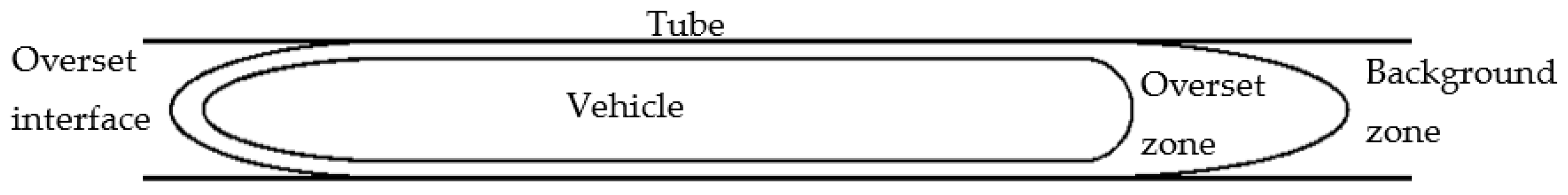
3. Numerical Simulations Using the 2-D URANS Model

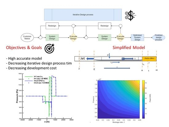
A 2-D CAD model, shown in Figure 4, was utilized to simulate the vehicle. The movement was applied to the overset cell zone to simulate the vehicle’s movement within the tube. The overset grid method [44,45,46] was implemented to generate the relative motion between the vehicle and the tube. Two subdomains share the computational domain (Figure 5): a stationary subdomain defined by the tube (Figure 5a) and a moving subdomain (Figure 5b) surrounding the vehicle in close proximity.

A structured grid was constructed using quadrilateral elements modeled by ANSYS ICEM Meshing tools. A background grid is defined as a cell zone with no boundary zone of type overset. The overset interface is used to pair multiple component grids with the background grid. The Metis-DR method [47] is utilized to allow parallel computations. The y+ value for the overset zone vehicle walls is 1, and that for the tube walls in the background zone is 2.

The solver setup for this simulation is a finite-volume 2-D space, density-based [48], unsteady, axisymmetric [49], flux-difference splitting ROE [50] with the implicit formulation. A second-order upwind [51] is used for the flow equations and turbulent closure models [52,53]. The energy equation is enabled. An ideal gas material model with viscosity–temperature relations governed by the Sutherland law is applied [54]. The flow conditions $p \mathrm{and} T$ are defined.

The tube and vehicle walls are adiabatic with no-slip conditions, and the tube portals are pressure inlet boundary types. The overset boundary type is assigned automatically when the overset interface is defined between the background and overset zones. Evaluation of the Knudsen number suggested continuum flow down to the finest grid size.

4. Results

In this section, the results for the developed algorithm are shown. These results are compared with the 2-D CFD analysis with the k-$\epsilon$ realizable model. The results are provided in the following sequence: the power required variations with the blockage ratio and different operating pressure, and various Mach numbers are studied. Then, we can illustrate the pressure coefficient distribution and the near-field flow characteristics. Following the URANS solution and flow-field predictions, a grid independency check is performed, and the results are illustrated by means of contour plots. Finally, the far-field results provide the time history for the flow-field pressure, velocity, and temperature distribution along the finite length of the tube.

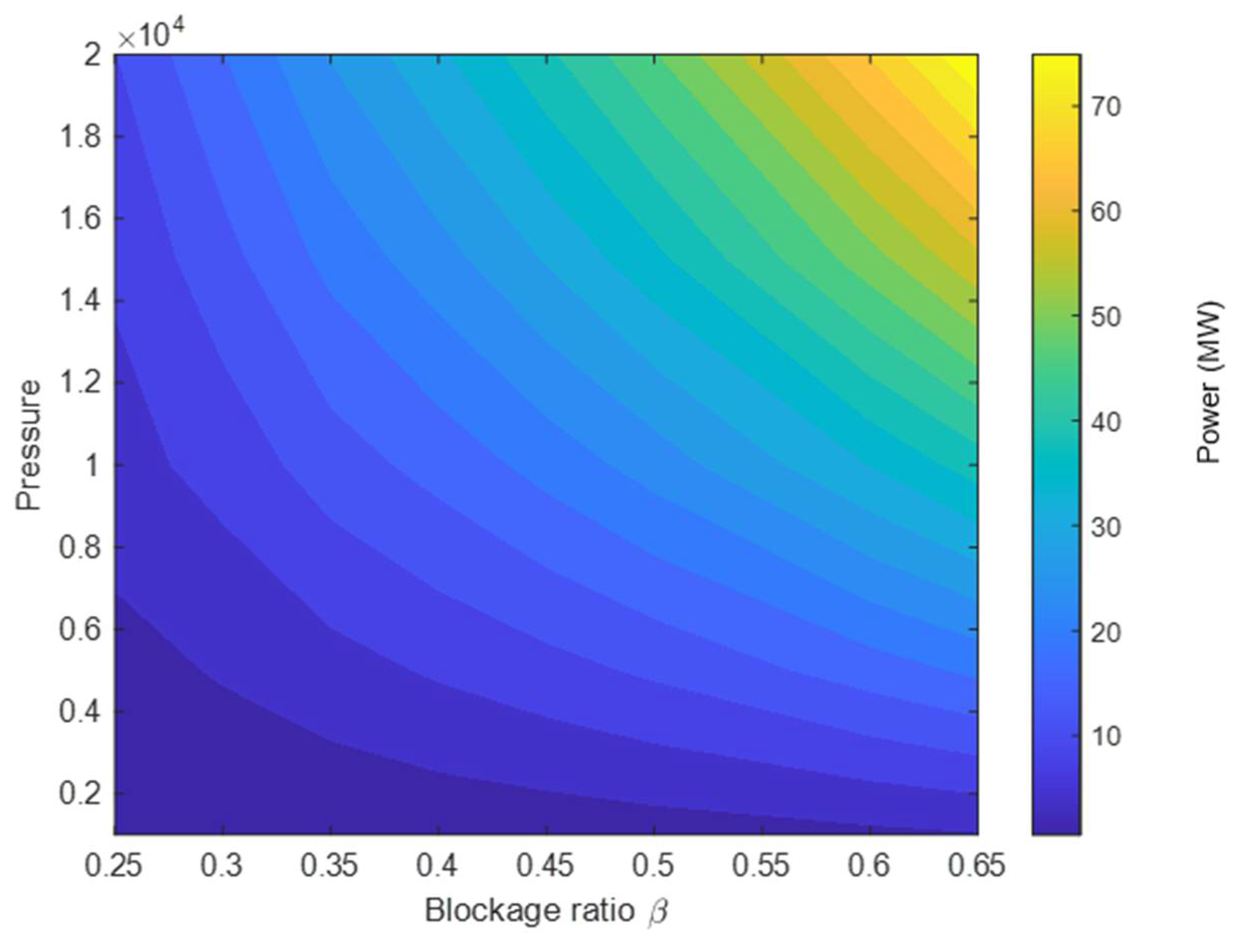
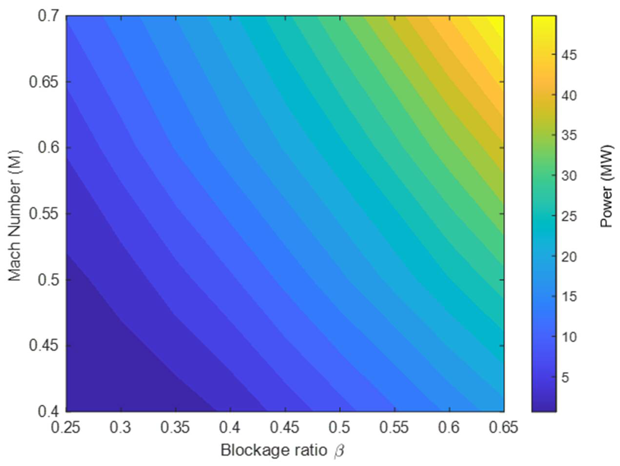
4.1. Power Estimations

Power estimation is pivotal to the design process of the vehicle. The Mach number, which represents the vehicle’s speed, is desired to be as high as possible. The blockage ratio is related to the vehicle and the tube diameters. The vehicle diameter is defined by the interior space required, while the tube diameter is desired to be as large as possible to reduce the blockage but as small as possible to reduce its cost. The vehicle’s surrounding pressure, i.e., the tube pressure, is desired to be as low as possible for drag reduction but as high as possible for safety reasons and vehicle heat rejection. These contradictory requirements demand intensive parametric studies to optimize the system’s aerodynamic performance.

Figure 6 shows the power map due to the vehicle drag, with the blockage ratio and operating pressure as variable parameters for a vehicle traveling at Mach 0.6, using the rapid 1-D algorithm described earlier. The maximum power occurs at a higher blockage ratio and pressure pair. The minimum power is as expected at a lower blockage ratio and pressure. The influence of the operating pressure effect is more dominant than the blockage effect for the lower blockage ratio values. However, for the high blockage ratio, the opposite trend is displayed.

Figure 7 shows the power variation for a fixed pressure of 10 kPa, with blockage ratio and Mach number variations. Similarly, the power increases with the blockage ratio and the Mach number as chocking in the passage is approached and causes a piston effect, causing a rapid increase in the pressure drag. The contours discussed are tools for a power-driven design. A limiting power range can be specified corresponding to a color code indicated in the graduated power column. The contours shown are two-dimensional slices of a broader three-dimensional performance map. A power value or range of values can be specified and displayed as a single three-dimensional surface, aiding the selection of optimum parameters of Mach number, block ratio, and pressure. Such elaborate contours are feasible to construct using the rapid technique presented here. Such construction utilizing CFD would require significant resources. Once the design parameters are selected, CFD is used to hone and fine-tune the final parameters. CFD studies are presented in the following sections and compared to the 1-D rapid results.

.

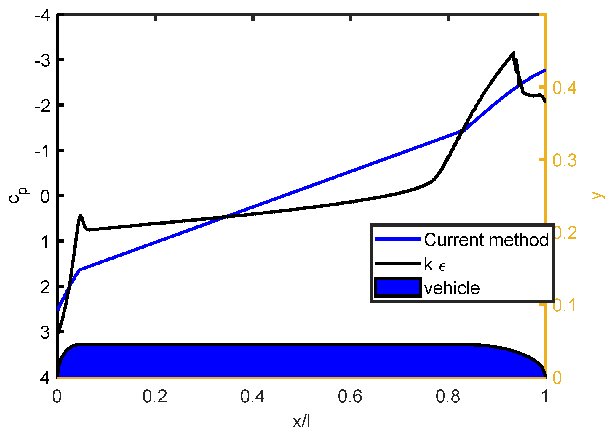
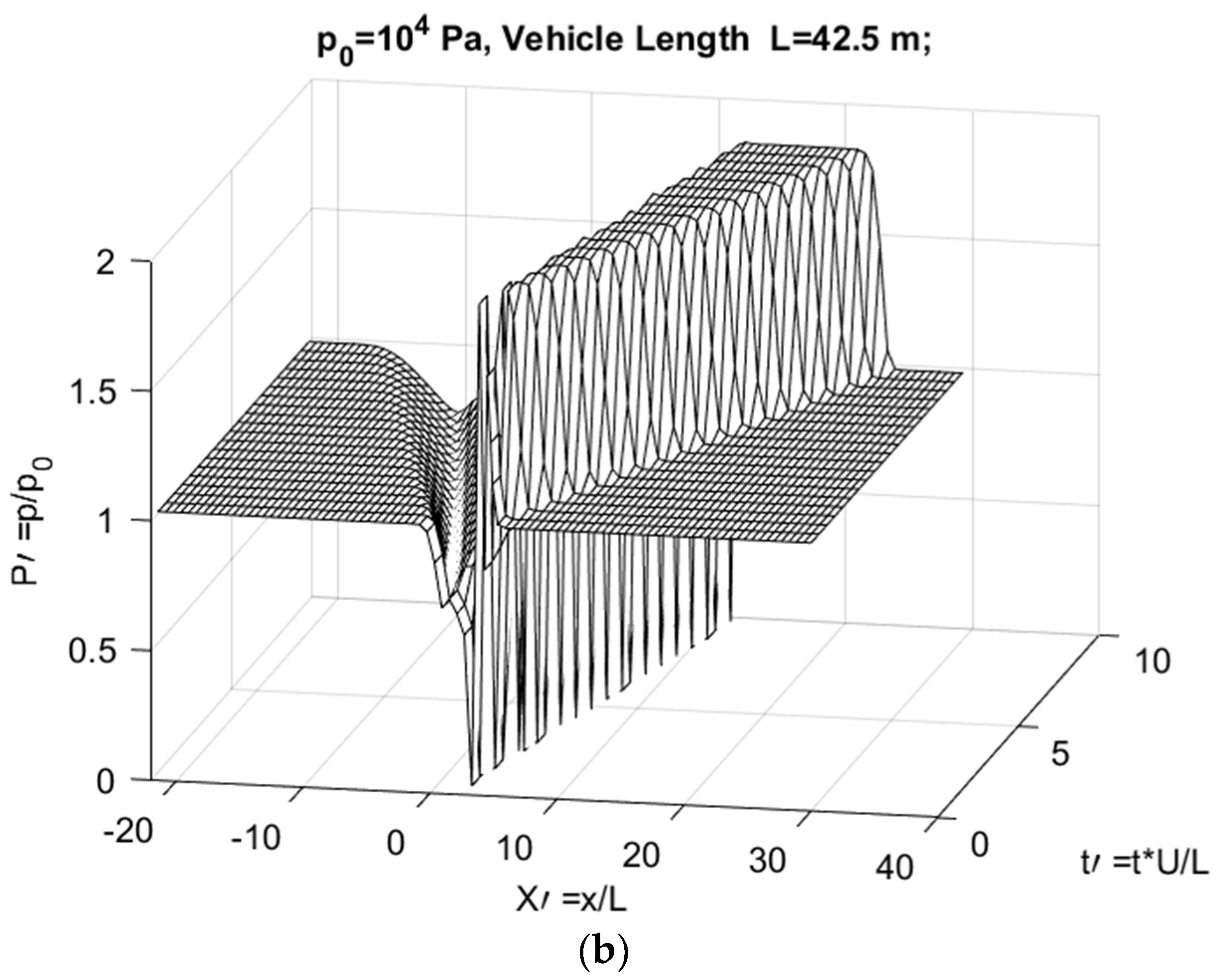
4.2. Near-Field Flow Results

Figure 8 shows the axisymmetric vehicle model and the near flow-field. The pressure coefficient distributions over the model using the developed algorithm and the CFD k-$\epsilon$ realizable turbulence model solution are compared. However, the developed algorithm is one-dimensional and naturally produces mean values for C_p. The current method provides an approximation for the near-field. However, the minimum and maximum pressure values are near the k-$\epsilon$ 2D results. The difference between the results shown in Figure 8 stems from the current model being 1-D, while the k-$\epsilon$ is 2-D.

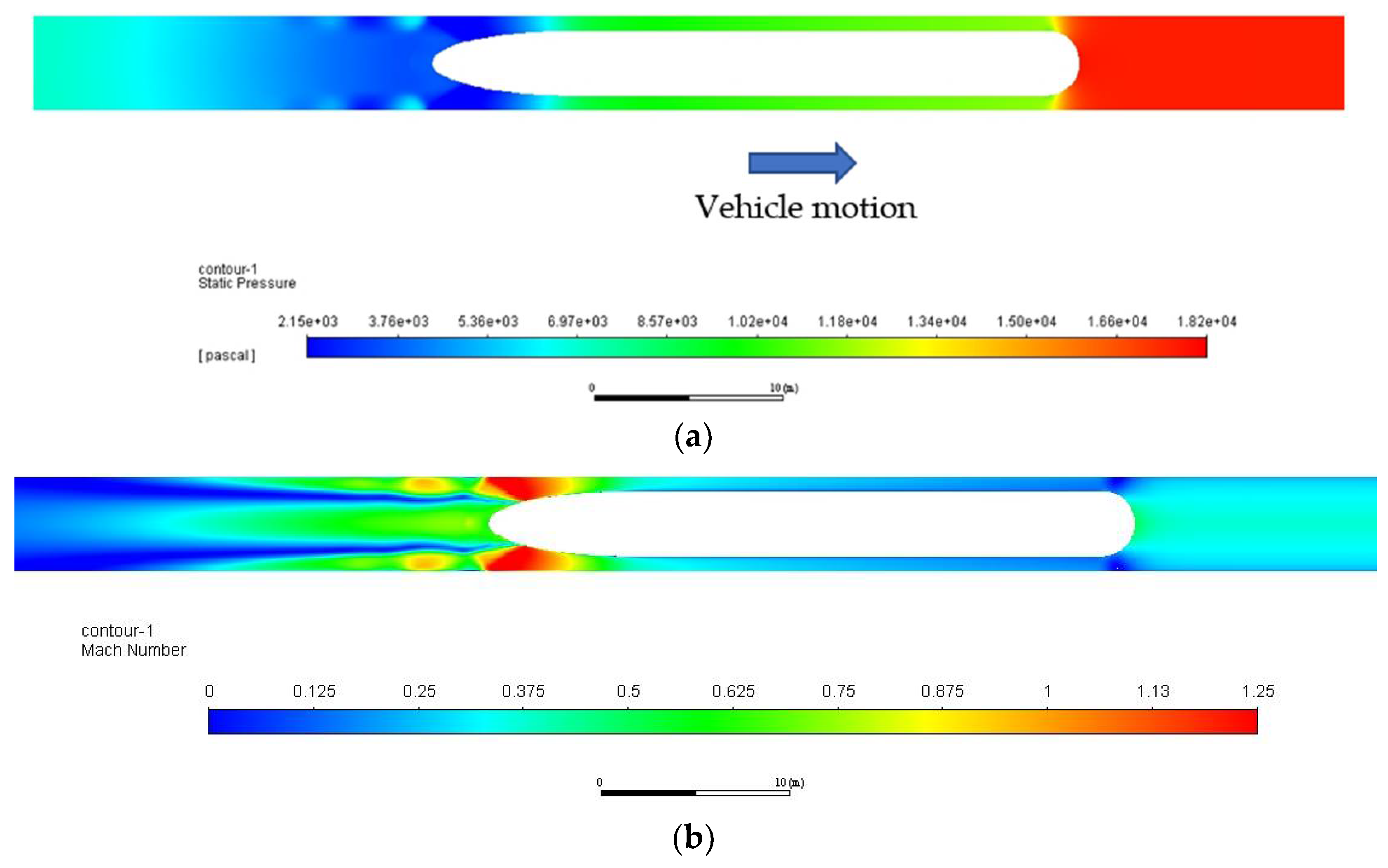
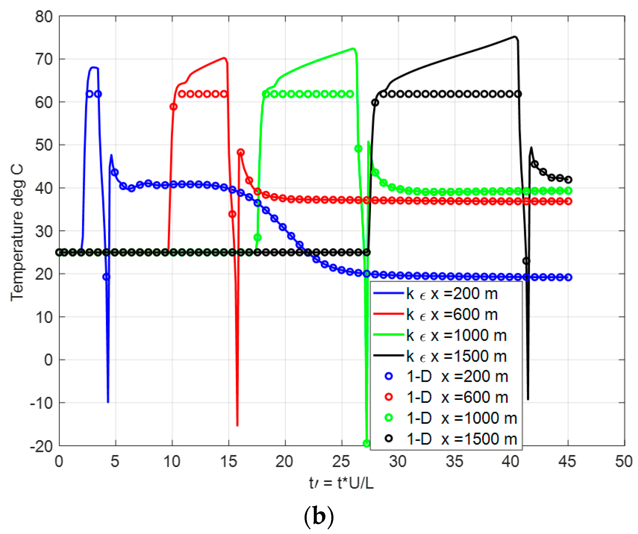
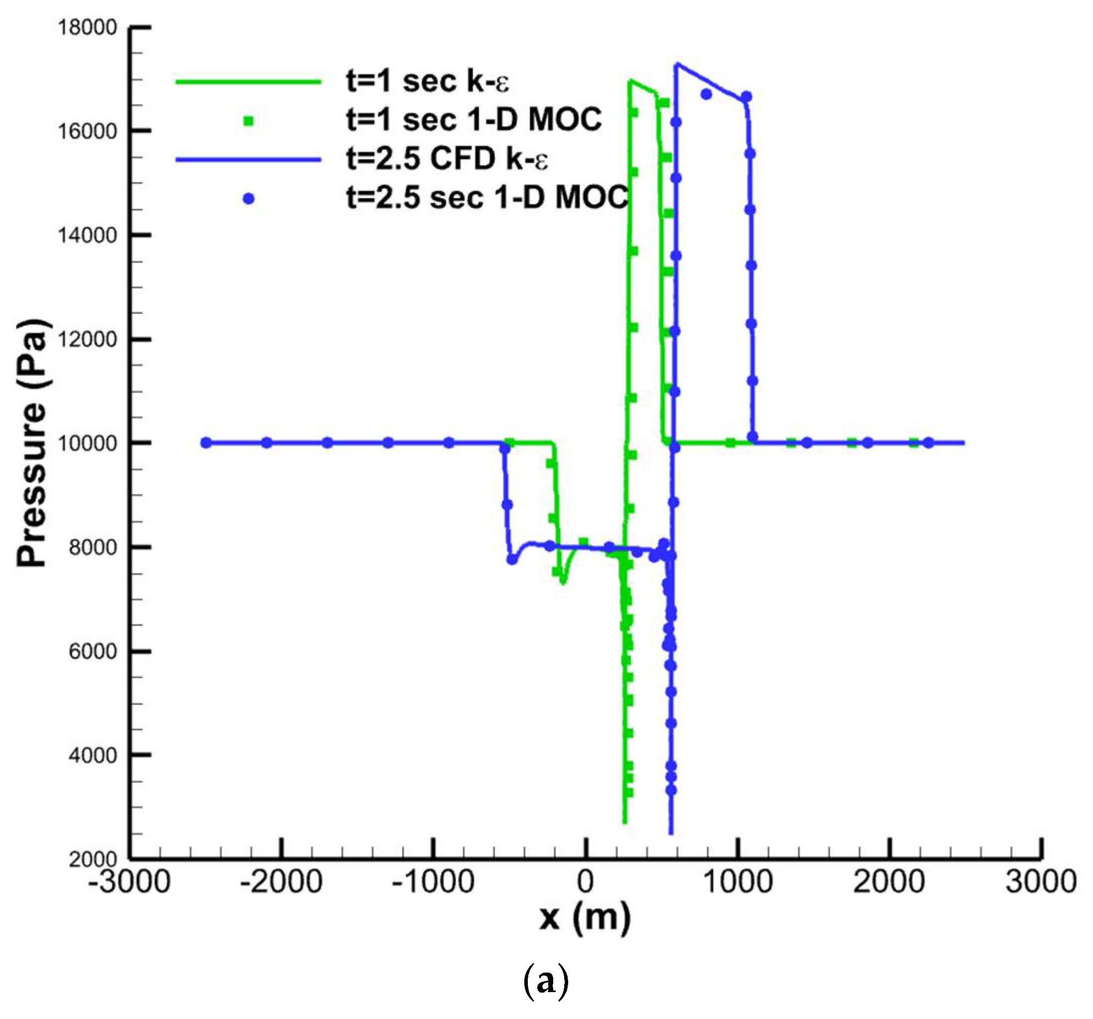
4.3. 2-D URANS Model Results

A grid convergence study is performed. The vehicle motion is repeated under coarse, medium, and fine meshes comprising 3.82 × 10⁵, 5.7 × 10⁵, and 1.05 × 10⁶ elements, respectively, as shown in

Table 2. Grid refinements.

	Overset Zone	Background Zone	Number of Elements
Coarse	50 × 150	50 × 7500	382,500
Medium	75 × 200	75 × 7500	577,500
Fine	100 × 500	100 × 10,000	1,050,000

. The pressure wave propagation along the tunnel is estimated utilizing these grid sizes. Figure 9 shows that fine and medium grid sizes have similar trends, but the coarse grid has a higher amplitude of the pressure value, at t = 1, 2.5 s. The coarse grid predictions agree with the other grid levels and are selected for further investigations due to the lower computational cost and time saving calculations.

Figure 10a indicates the static pressure contour around the vehicle. The pressure is exceptionally high downstream (red colormap) and expanded into the left. The calculations performed by MOC show a value of 23 KN. Figure 10b reveals the high Mach number experienced at the rear part of the vehicle due to flow expansion.

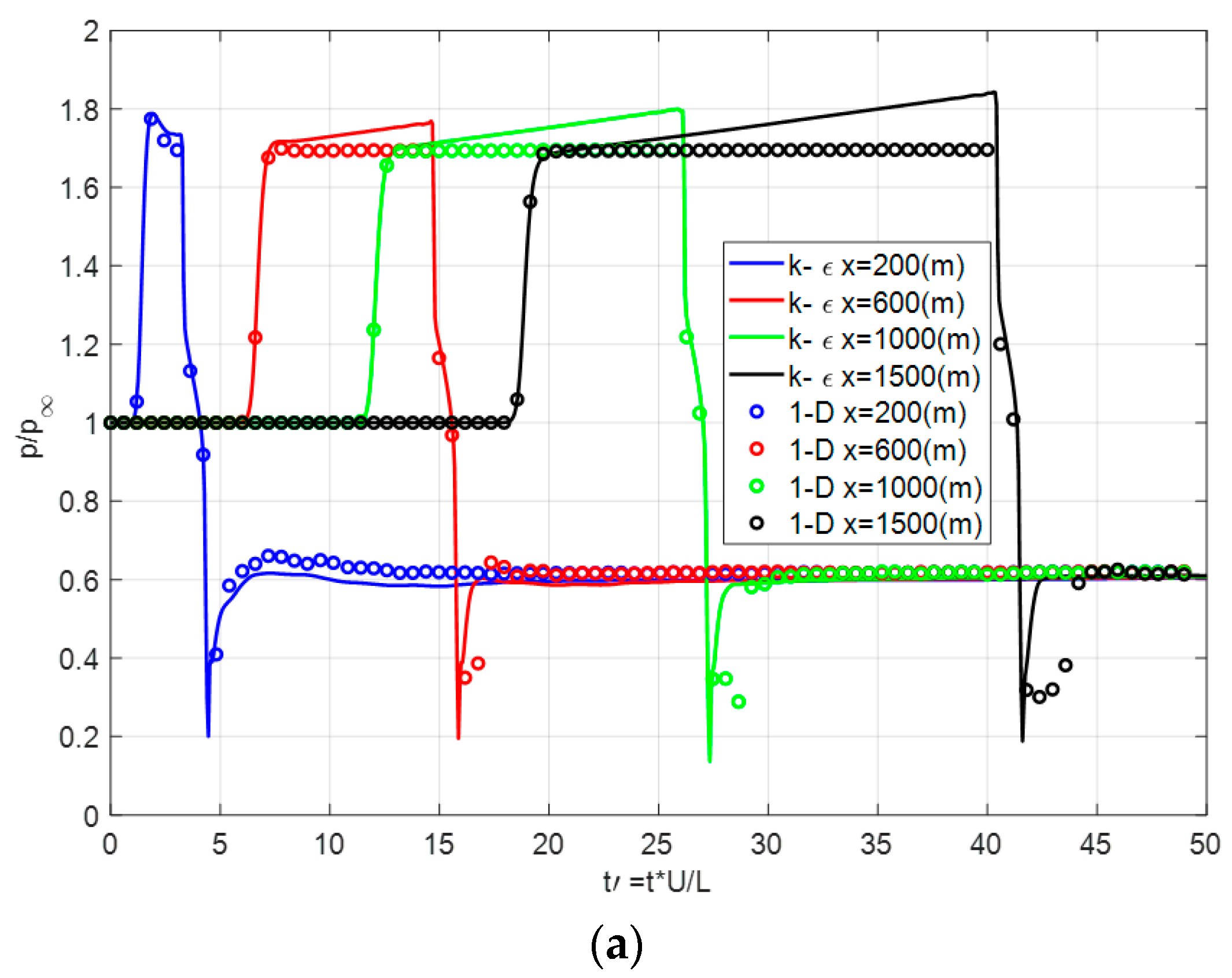
4.4. Comparing the Developed Algorithm with the 2-D CFD Model

The far-field flow solution for the compression wave propagation along the tube requires a time–space-dependent solution. The methods described in Section 1 for the 1-D algorithm solutions support a time history for the flow-field variables. The new algorithm results were compared with an unsteady turbulent k-ε model. Obtained results agree in predicting the pressure wave and flow properties’ distribution along with the tube domain. For the near-field flow properties around the vehicle, Figure 11 shows the time history for pressure (a) and temperature (b) measurements monitored using artificial probes fixed at different x-locations along the tube (x = 200, 600, 1000, 1500 m). URANS results are in excellent agreement with the developed algorithm. The 1-D algorithm and URANS estimate the temperature variations at prescribed locations. The numerical results agree very well, but the 1-D provides a lower maximum pressure and temperature value than the turbulent model of k-ε The temperature measurement shows a maximum of around 72 °C, which means that a higher operating temperature is expected. The system is adiabatic, and no heat source is defined. The temperature variation generated from the flow-field area changes and the domain’s expansion/compression causes the waves’ appearance. Another explanation as to why the turbulence model of k-ε expects a higher temperature may be that also the viscous dissipation into thermal energy is the source of the higher temperature levels shown in Figure 11b [53].

Figure 12a,b show the pressure wave propagation in space and time. Figure 12a shows the pressure wave propagation at two flow times. During the flow time = 1 s, the developed algorithm and the CFD solutions for the pressure wave propagation predict that the propagation distance lies near 300 (m), which ($7.3 \mathrm{L}$), but at t = 2.5, the wave propagates to more extended spaces, almost twice the previous wave propagating period (15 L). The good agreement between the developed algorithm and the 2-D URANS provides high robustness for the model, requiring less computing time for the rapid prediction of the flow-field of high-speed vehicles traveling in a tube. The current method’s computational time is negligible compared to the complex grid motion applied to generate the results of the k-ε model. The computational time calculated with different grid sizes is shown clearly in

Table 3. Comparison of computational time for 1-sec travel time.

		Calculation Time for 1 s Motion	Difference in Drag Force Estimations (Compared with Fine Grid)
CFD	Coarse grid	24 h	96%
	Medium grid	28 h	97%
	Fine grid	32 h	-
1-D Method of Characteristics (current)		15 min	95%

below.

The 1-D Method of Characteristics’ challenges includes selecting suitable boundary conditions and coupling between the near-field and far-field flow regimes. The near-field flow solver could extend to a higher order to improve the accuracy, but the numerical budget would increase substantially. In contrast, the current method is simple and provides greater than 95% accuracy compared to the more complex solution utilizing the k ϵ model.

5. Conclusions

The introduction of Hyperloop has increased the interest in rapid land transportation technology, but the near-space pressure level is of concern regarding safety and cost. A tube pressure range comparable to flight conditions is studied to tackle the significant challenges in designing such a vehicle and predicting its motion. In this paper, we developed an algorithm employing an in-house code for near-field and far-field analysis utilizing Reimann numerical schemes. The developed algorithm was tested against 2-D CFD modeling and produced similar results. The benefits of rapid flow models include a decreased computational burden. The complete flow-field solution was acquired in less time than the URANS simulations, which require a complex gird and mesh motion to capture the flow-field accurately, and it allows parametric studies of a large number of vehicle flow conditions deemed necessary for system design. Such simplified, low-cost tools have been developed and shown to decrease the design and development costs of the vehicle–tube system.

The aerodynamic drag and power levels related to blockage effects and operating pressure were also presented, including power contours. The power increases with the blockage ratio, operating pressure, and Mach number. The time-varying solution for the flow-field captures the long-distance wave propagation.

References

1. Foa, J.V. Transfortation Means and Method; Springer: Berlin/Heidelberg, Germany, 1965. [Google Scholar]
2. Woods, W.A.; Pope, C.W. A Generalised Flow Prediction Method for the Unsteady Flow Generated by a Train in a Single-Track Tunnel. J. Wind Eng. Ind. Aerodyn. 1981, 7, 331–360. [Google Scholar] [CrossRef]
3. Hammitt, A.G. Aerodynamics of Vehicles in Finite Length Tubes; No. FRA-ORD&D-74-10; Federal Railroads Administration: Washington, DC, USA, 1974.
4. Hammitt, A.G. Aerodynamic Analysis of Tube Vehicle Systems. AIAA J. 1972, 10, 282–290. [Google Scholar] [CrossRef]
5. Ross, P.E. Hyperloop: No Pressure: The Vacuum Train Project Will Get Its First Test Track This Year. IEEE Spectr. 2016, 53, 51–54. [Google Scholar] [CrossRef]
6. Noh, H.M. Wind Tunnel Test Analysis to Determine Pantograph Noise Contribution on a High-Speed Train. Adv. Mech. Eng. 2019, 11, 1–11. [Google Scholar] [CrossRef] [Green Version]
7. Yang, M.; Du, J.; Li, Z.; Huang, S.; Zhou, D. Moving Model Test of High-Speed Train Aerodynamic Drag Based on Stagnation Pressure Measurements. PLoS ONE 2017, 12, e0169471. [Google Scholar] [CrossRef]
8. Lluesma-Rodríguez, F.; González, T.; Hoyas, S. CFD Simulation of a Hyperloop Capsule inside a Closed Environment. Results Eng. 2021, 9, 2020–2022. [Google Scholar] [CrossRef]
9. Khayrullina, A.; Blocken, B.; Janssen, W.; Straathof, J. CFD Simulation of Train Aerodynamics: Train-Induced Wind Conditions at an Underground Railroad Passenger Platform. J. Wind Eng. Ind. Aerodyn. 2015, 139, 100–110. [Google Scholar] [CrossRef]
10. Zhou, P.; Zhang, J.; Li, T.; Zhang, W. Numerical Study on Wave Phenomena Produced by the Super High-Speed Evacuated Tube Maglev Train. J. Wind Eng. Ind. Aerodyn. 2019, 190, 61–70. [Google Scholar] [CrossRef]
11. Riva, N.; Benedetti, L.; Sajó, Z. Modeling the Hyperloop with COMSOL Multiphysics®: On the Aerodynamics Design of the EPFLoop Capsule. In Proceedings of the 2018 COMSOL Conference, Lausanne, Switzerland, 22–24 October 2018; pp. 1–7. [Google Scholar]
12. Opgenoord, M.M.J.; Caplan, P.C. On the Aerodynamic Design of the Hyperloop Concept. In Proceedings of the 35th AIAA Applied Aerodynamics Conference 2017, Denver, CO, USA, 5–9 June 2017; pp. 1–16. [Google Scholar] [CrossRef] [Green Version]
13. Sui, Y.; Niu, J.; Ricco, P.; Yuan, Y.; Yu, Q.; Cao, X.; Yang, X. Impact of Vacuum Degree on the Aerodynamics of a High-Speed Train Capsule Running in a Tube. Int. J. Heat Fluid Flow 2021, 88, 108752. [Google Scholar] [CrossRef]
14. Opgenoord, M.M.; Caplan, P. MIT Hyperloop Final Report. MIT Hyperloop Team 2017, 134. [Google Scholar]
15. Oh, J.S.; Kang, T.; Ham, S.; Lee, K.S.; Jang, Y.J.; Ryou, H.S.; Ryu, J. Numerical Analysis of Aerodynamic Characteristics of Hyperloop System. Energies 2019, 12, 518. [Google Scholar] [CrossRef] [Green Version]
16. Decker, K.; Chin, J.; Peng, A.; Summers, C.; Nguyen, G.; Oberlander, A.; Sakib, G.; Sharifrazi, N.; Heath, C.; Gray, J.; et al. Conceptual Feasibility Study of the Hyperloop Vehicle for Next-Generation Transport. In Proceedings of the AIAA SciTech Forum—55th AIAA Aerospace Sciences Meeting, AIAA 2017-0221, Grapevine, TX, USA, 9–13 January 2017; pp. 1–22. [Google Scholar] [CrossRef]
17. Raghunathan, R.S.; Kim, H.D.; Setoguchi, T. Aerodynamics of High-Speed Railway Train. Prog. Aerosp. Sci. 2002, 38, 469–514. [Google Scholar] [CrossRef]
18. Kim, T.K.; Kim, K.H.; Kwon, H. Bin Aerodynamic Characteristics of a Tube Train. J. Wind Eng. Ind. Aerodyn. 2011, 99, 1187–1196. [Google Scholar] [CrossRef]
19. Jang, K.S.; Le, T.T.G.; Kim, J.; Lee, K.S.; Ryu, J. Effects of Compressible Flow Phenomena on Aerodynamic Characteristics in Hyperloop System. Aerosp. Sci. Technol. 2021, 117, 106970. [Google Scholar] [CrossRef]
20. Kang, H.; Jin, Y.; Kwon, H.; Kim, K. A Study on the Aerodynamic Drag of Transonic Vehicle in Evacuated Tube Using Computational Fluid Dynamics. Int. J. Aeronaut. Sp. Sci. 2017, 18, 614–622. [Google Scholar] [CrossRef]
21. Kollmann, W. Computational Fluid Dynamics, Vki-Book; Hemisphere Publishing Corp.: Washington, DC, USA, 1980; Volume 2, ISBN 3804204422. [Google Scholar]
22. Lluesma-Rodríguez, F.; González, T.; Hoyas, S. Cfd Simulation of a Hyperloop Capsule inside a Low-Pressure Environment Using an Aerodynamic Compressor as Propulsion and Drag Reduction Method. Appl. Sci. 2021, 11, 3934. [Google Scholar] [CrossRef]
23. Rivero, J.M.; González-Martínez, E.; Rodríguez-Fernández, M. Description of the Flow Equations around a High Speed Train inside a Tunnel. J. Wind Eng. Ind. Aerodyn. 2018, 172, 212–229. [Google Scholar] [CrossRef]
24. Rodríguez-, M.; Rivero, J.M.; Gonz, E.; González-Martínez, E.; Rodríguez-Fernández, M. A Methodology for the Prediction of the Sonic Boom in Tunnels of High-Speed Trains. J. Sound Vib. 2019, 446, 37–56. [Google Scholar] [CrossRef]
25. Gilbert, T.; Baker, C.; Quinn, A. Aerodynamic Pressures around High-Speed Trains: The Transition from Unconfined to Enclosed Spaces. Proc. Inst. Mech. Eng. Part F J. Rail Rapid Transit 2013, 227, 609–622. [Google Scholar] [CrossRef]
26. William-Louis, M.; Tournier, C. A Wave Signature Based Method for the Prediction of Pressure Transients in Railway Tunnels. J. Wind Eng. Ind. Aerodyn. 2005, 93, 521–531. [Google Scholar] [CrossRef]
27. Hammitt, A.G. Unsteady Aerodynamics of Vehicles in Tubes. AIAA J. 1975, 13, 497–501. [Google Scholar] [CrossRef]
28. Sajben, M. Fluid Mechanics of Train-Tunnel Systems in Unsteady Motion. AIAA J. 1971, 9, 1538–1545. [Google Scholar] [CrossRef]
29. Sugimoto, N. Acoustic Analysis of the Pressure Field Generated by Acceleration of a Train in a Long Tunnel. J. Comput. Acoust. 1999, 7, 207–224. [Google Scholar] [CrossRef]
30. Fukuda, T.; Ozawa, S.; Iida, M.; Takasaki, T.; Wakabayashi, Y. Distortion of Compression Wave Propagating through Very Long Tunnel with Slab Tracks. JSME Int. J. Ser. B Fluids Therm. Eng. 2007, 49, 1156–1164. [Google Scholar] [CrossRef] [Green Version]
31. Miyachi, T.; Ozawa, S.; Fukuda, T.; Iida, M. A New Simple Equation Governing Distortion of Compression Wave Propagating Through Shinkansen Tunnel with Slab Tracks. J. Fluid Sci. Technol. 2013, 8, 60–73. [Google Scholar] [CrossRef] [Green Version]
32. Miyachi, T.; Saito, S.; Fukuda, T.; Sakuma, Y.; Ozawa, S.; Arai, T.; Sakaue, S.; Nakamura, S. Propagation Characteristics of Tunnel Compression Waves with Multiple Peaks in the Waveform of the Pressure Gradient: Part 1: Field Measurements and Mathematical Model. Proc. Inst. Mech. Eng. Part F J. Rail Rapid Transit 2015, 230, 1297–1308. [Google Scholar] [CrossRef]
33. Aoki, T.; Yamamoto, J.; Nagatani, K. Characteristics of a Compression Wave Propagating over Porous Plate Wall in a High-Speed Railway Tunnel. J. Therm. Sci. 2008, 17, 218–223. [Google Scholar] [CrossRef]
34. Akbari, P.; Bermudes, L. Shock Waves in Narrow Channels and Their Applications for High-Efficiency Unsteady Wave Engines. SAE Tech. Pap. 2017. [Google Scholar] [CrossRef]
35. Chen, C.-H.; Lee, L.H. Computing Budget Allocation. In Stochastic Simulation Optimization; World Scientific Publishing Co Pte Ltd.: Singapore, 2010; pp. 15–28. [Google Scholar] [CrossRef]
36. Baron, A.; Mossi, M.; Sibilla, S. The Alleviation of the Aerodynamic Drag and Wave Effects of High-Speed Trains in Very Long Tunnels. J. Wind Eng. Ind. Aerodyn. 2001, 89, 365–401. [Google Scholar] [CrossRef]
37. Kim, J.; Jang, K.S.; Le, T.T.G.; Lee, K.S.; Ryu, J. Theoretical and Numerical Analysis of Pressure Waves and Aerodynamic Characteristics in Hyperloop System under Cracked-Tube Conditions. Aerosp. Sci. Technol. 2022, 123, 107458. [Google Scholar] [CrossRef]
38. Transportation, M.; Wu, C.; Gao, X.; Gao, P. Characteristic Analysis of Air Pressure Wave Generated by High-Speed Trains Traveling through a Tunnel. J. Mod. Transp. 2012, 20, 31–35. [Google Scholar] [CrossRef] [Green Version]
39. Miyachi, T. Acoustic Model of Micro-Pressure Wave Emission from a High-Speed Train Tunnel. J. Sound Vib. 2017, 391, 127–152. [Google Scholar] [CrossRef]
40. Zhao, Y.; Zhang, J.; Li, T.; Zhang, W. Aerodynamic Performances and Vehicle Dynamic Response of High-Speed Trains Passing Each Other. J. Mod. Transp. 2012, 20, 36–43. [Google Scholar] [CrossRef] [Green Version]
41. Alsawy, T.; Abdel Gawad, A.F. Effect of Twist of a Wide-Chord Fan-Blade on the Aerodynamic Performance of the Fan of a High-Bypass Turbofan Engine. In Proceedings of the Thirteenth International Conference of Fluid Dynamics, Cairo, Egypt, 21–22 December 2018; ICFD13-EG-6S01. [Google Scholar]
42. Chan, W.M.; Gomez, R.J., III; Rogers, S.E.; Buning, P.G. Best Practices in Overset Grid Generation. In Proceedings of the 32nd AIAA Fluid Dynamics Conference, St. Louis, MI, USA, 24–26 June 2002. AIAA paper 2002-3191. [Google Scholar]
43. Chan, W.M. Advances in Software Tools for Pre-Processing and Post-Processing of Overset Grid Computations. In Proceedings of the 9th International Conference on Numerical Grid Generation in Computational Field Simulations, San Jose, CA, USA, 11–18 June 2005; pp. 1–8. [Google Scholar]
44. Le, T.T.G.; Jang, K.S.; Lee, K.S.; Ryu, J. Numerical Investigation of Aerodynamic Drag and Pressurewaves in Hyperloop Systems. Mathematics 2020, 8, 1973. [Google Scholar] [CrossRef]
45. Scheidegger, T. Overset Meshing in ANSYS Fluent; ANSYS Inc.: Canonsburg, PA, USA, 2016. [Google Scholar]
46. Nerinckx, K.; Vierendeels, J.; Dick, E. A Mach-Uniform Pressure-Correction Algorithm with AUSM+ Flux Definitions. Int. J. Numer. Methods Heat Fluid Flow 2006, 16, 718–739. [Google Scholar] [CrossRef]
47. Bardina, J.E.; Huang, P.G.; Coakley, T.J. Turbulence Modeling Validation. In Proceedings of the 28th Fluid Dynamics Conference, Snowmass Village, CO, USA, 29 June–2 July 1997. [Google Scholar] [CrossRef]
48. Toro, E.F. Riemann Solvers and Numerical Methods for Fluid Dynamics; Springer Science & Business Media: Berlin/Heidelberg, Germany, 2009; ISBN 9783540252023. [Google Scholar]
49. Hussaini, M.Y.; van Leer, B.; Van Rosendale, J. Upwind and High-Resolution Schemes; Springer Science & Business Media: Berlin/Heidelberg, Germany, 2012; ISBN 9783642644528. [Google Scholar]
50. Bose, A.; Viswanathan, V.K. Mitigating the Piston Effect in High-Speed Hyperloop Transportation: A Study on the Use of Aerofoils. Energies 2021, 14, 464. [Google Scholar] [CrossRef]
51. Wong, F.T. Aerodynamic Design and Optimization of a Hyperloop Vehicle; TU Delft: Delft, The Netherlands, 2018. [Google Scholar]
52. Herrmann Schlichting, K.G. Boundary-Layer Theory; Springer: Berlin Heidelberg, Germany, 2000; ISBN 9783642858314. [Google Scholar]
53. Pope, S.B. Turbulent Flows; Cambridge University Press: Cambridge, UK, 2000; Volume 13. [Google Scholar]
54. Bertin, J.J.; Smith, M.L. Aerodynamics for Engineers, 6th ed.; Pearson Education Limited: Edinburgh, UK, 2014; Volume 3, ISBN 10: 0-273-79327-6. [Google Scholar]
Figure 1. (a) Pod and cabin detailed views; (b) simplified 2-D pod configurations.
Energies 15 06074 g001
Figure 2. Sketch diagram for pod motion in a tube.
Energies 15 06074 g002
Figure 3. The modeled near-field domain.
Energies 15 06074 g003
Figure 4. Overset boundary zone and interface.
Energies 15 06074 g004
Figure 5. Background and overset grid concept; only a fraction of the tube domain is shown. (a) 75 × 7500 background grid (stationary); (b) 50 × 200 moving domain (overset domain); (c) overlaying the overset domain on the background domain.
Energies 15 06074 g005
Figure 6. Effect of blockage ratio on vehicle’s power at various operating pressures, M = 0.6.
Energies 15 06074 g006
Figure 7. Power contours correlating blockage ratio β and Mach number, p = 10   kPa .
Energies 15 06074 g007
Figure 8. Pressure coefficient C p distribution at t = 1 s, M = 0.6, p = 10 kPa, β = 0.56 .
Energies 15 06074 g008
Figure 9. Pressure distribution at y = 2 m (between the tube and the vehicle), t = 1, 2.5 s, with different grids using the k- ε realizable model. The pressure and Mach number contours provided in Figure 10 were obtained with the k-ε turbulent model. The solution represents a compression in front of the vehicle that causes the “piston effect” [52].
Energies 15 06074 g009
Figure 10. (a) Static pressure; (b) Mach Number contour, t = 6.33 s (M = 0.6, β = 0.56).
Energies 15 06074 g010
Figure 11. (a) Pressure ratio, (b) temperature history reported at x = 200, 600, 1000, 1500 (m) β = 0.56 .
Energies 15 06074 g011aEnergies 15 06074 g011b
Figure 12. Pressure wave propagation (a) along x-coordinates at t = 1, 2.5 s; (b) wave propagation in x-space and time, β = 0.56 .
Energies 15 06074 g012aEnergies 15 06074 g012b