Effectiveness of Energy Transfer versus Mixing Entropy in Coupled Mechanical–Electrical Oscillators

Abstract

Electrostatic energy harvesters convert kinetic energy into electrical energy via variable capacitors. Efforts to improve their power output are hampered by a lack of understanding of the fundamental limit for energy conversion efficiency. In heat engines, the theoretical limit of conversion efficiency is intrinsically related to entropy and the second law of thermodynamics. Laying the foundation for similar concepts for kinetic energy harvesters may be necessary for establishing a conversion efficiency limit. Thus, the mixing entropy concept is borrowed from statistical mechanics and is adapted here, for the first time, to characterize the energy transfer between coupled mechanical–electrical oscillators. The investigated system is composed of a spring-mass coupled to an inductance-capacitor circuit via a variable capacitor. Combining the two subsystems (electrical and mechanical) generates entropy, referred to as mixing entropy. A non-dimensional study of the governing equations of the systems and their energy terms is carried out. Trends in mixing entropy are compared with trends in the total energy of the system, assuming a conservative system, weak coupling between electrical and mechanical domains, and identical natural frequency of the two oscillators. It is found that mixing entropy can predict the peak in effectiveness of the energy transfer between the two domains. For the cases studied, the maximum mixing entropy and effectiveness values occur when the ratio of the mechanical domain energy to the total energy of the system is 67%. The maximum effectiveness is independent of the initial conditions and depends on the squared ratio of the natural frequency of the nominal coupling capacitor to the natural frequency of the mechanical system.

1. Introduction

Ambient vibrational energy remains the most popular source of energy harvesting to power miniaturized sensors in a variety of applications. Ambient vibrational energy is converted into electricity via electromagnetic, piezoelectric, or electrostatic transduction. All kinetic commercial harvesters are based on the first two transduction mechanisms. Examples include the electromagnetic generators from XIDASIOT [1] or EnOcean [2], and piezoelectric generators from MIDE technologies [3] or Piezo [4]. Electrostatic harvesters, based on microscale variable capacitors, are still in the research phase as their performance is not yet adequate for existing power needs. A variety of methods are being explored to increase the power output of this type of generator, including impact-based harvesters [5,6,7,8], parallel coupling [9], and novel device geometries [10,11,12]. However, a common drawback remains the lack of understanding of the parameters that control the fundamental theoretical limit for power conversion. In fact, a standard metric to gauge the performance of electrostatic harvesters has yet to emerge, although various parameters such as efficiency, effectiveness, or figure-of-merit have been proposed in the past [5,6]. In line with this, Roundy [13] proposed an effectiveness formula applicable to electrostatic harvesters. However, the defined effectiveness still depends on a coupling coefficient term, a quality factor, and a baseline material density term, which may not give the necessary insight into the maximum possible power to be harvested. Halvorsen [14] penned a letter to address the issue of performance close to the fundamental limit of electrostatic energy harvesters, but it still fell short in providing a clear fundamental limit of the energy transfer from mechanical to electrical domains. Toshiyoshi et al. [15] presented an extended discussion of the effectiveness of energy harvesters, including damping terms, without giving a clear limit of the harvested mechanical energy. In general, while all these works show a good understanding of the coupling between the mechanical and the electrical systems, the damping effect, and the parameters necessary for improving the power harvested by those devices, there is still a need to obtain an actual theoretical maximum value of energy that can be harvested from a specific mechanical vibration energy input. Other energy conversion systems are characterized by efficiency with an established theoretical limit. For example, that is set by Carnot efficiency for heat engines [16], or by the Betz limit for wind turbines [17]. Similar to the Carnot efficiency [18], a fundamental limit will always involve the study of a reversible system without losses, as this system’s efficiency can never be lower than any irreversible system’s efficiency [19,20]. Entropy and the second law of thermodynamics play a key role in establishing the fundamental limit of energy conversion efficiency in both heat engines and wind turbines, and as such, its concept has been extended to other engineering fields such as fluid mechanics, electricity [19,21], information theory [22], mechanical vibrations [23], and statistical energy analysis [24]. Thus, exploring an entropy-like concept for vibrational to electric energy conversion systems might prove to be useful in establishing a fundamental limit for energy conversion and this task is undertaken here.

Electrostatic vibration energy harvesters are based on the principle of a capacitance variation between two electrodes subjected to external vibrations [25]. Multiple structures have been proposed for electrostatic energy harvesters, as the capacitance can be changed by either varying the distance between two electrodes [26], the electrodes overlapping area [12], or the dielectric [27] between the two electrodes based on the parallel plate capacitance formula [28]. Electrostatic energy harvesters are, in essence, coupled electro-mechanical oscillators somewhat similar to those described in the next section. Power flow in coupled oscillators has been investigated since the early 1960s. Lyon and Maidanik were the first to propose the heat flow analogy in the treatment of this problem [29]. Later, Carcaterra, in a pioneering work, proposed an entropy-based formulation of the power flow in coupled mechanical oscillators [30], defining the oscillator’s entropy based on its average modal energy. The approach was then extended to a statistical energy analysis [31]. Recently, Tufano and Sotoudeh added to this framework, proposing the new concept of mixing entropy, which is the entropy generated due to the coupling of vibrating subsystems [32,33].

This paper adapts and explores, for the first time, the concept of mixing entropy in the context of coupled mechanical–electrical oscillators employing variable capacitors as coupling elements. Trends in the effectiveness of the energy transfer between the two oscillators are investigated in terms of initial energies and system characteristics alongside changes in mixing entropy. The present study considers conservative, non-damped oscillators with a bidirectional power flow, i.e., no power is extracted from the electrical system. The mixing entropy concept explored here indicates that its maximum value coincides with the maximum effectiveness value of the ideal electromechanical system considered in this paper. Thus, using the mixing entropy can predict the maximum effectiveness of an ideal electrostatic energy harvester. This study paves the way for further investigations of dissipative systems with energy extraction, laying down the foundations for future work on establishing energy conversion limits in electrostatic harvesters.

2. System and Governing Equations

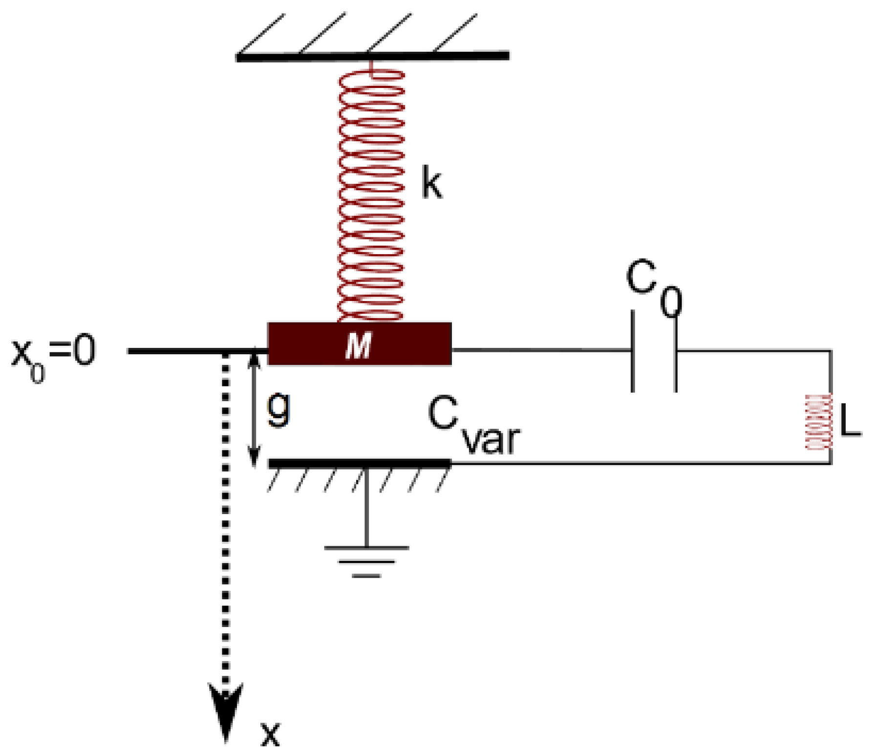
2.1. System Description

Figure 1 shows the system under consideration. It consists of a mechanical oscillator of mass $M$ connected to a clamped end by a linear spring of stiffness $k$. This is coupled to an electrical oscillator of inductance $L$ and capacitance $C_0$. The coupling element is a variable capacitor $C_{var}$. The mass $M$ of the mechanical oscillator acts as the moving electrode of the variable capacitor. As the mass moves up and down, the mechanical forces work against the electrostatic force and vice versa, resulting in an energy transfer from the mechanical to the electrical domains. This system is the idealized, damping-free, and simplified version of the mechanical–electrical coupled oscillators found in electrostatic energy harvesters.

2.2. Governing Equations

Applying Newton’s second law of motion to the mechanical system and Kirchhoff’s law to the electrical system, the governing equations are as follows:

$$m\ddot{x}+kx-\frac{1}{2}\frac{q^2}{\epsilon A}=0$$

(1)

$$L\ddot{q}+\frac{q}{C_0}-q\frac{\left(x-g\right)}{\epsilon A}=0$$

(2)

The unstretched position of the spring, $x_0$, is set as the origin of the system of coordinates. Thus, $x$ is the mass displacement. When the spring is unstretched, the variable capacitor plates are at the nominal distance, $g$. The instantaneous charge in the electrical system is $q$. The permittivity of the dielectric and the area of the variable capacitor are ε and $A$, respectively. For all of the results presented, the governing equations were solved for non-zero initial displacement, $x_i$, and initial charge, $q_i$, and zero initial velocity and current, ${\dot{x}}_i$ and ${\dot{q}}_i$, respectively.

2.3. Normalized Governing Equations

To better understand the relationship between effectiveness and the other parameters of the system, the governing equations are normalized. The coordinate $x$ is normalized to the static equilibrium gap of the variable capacitor, $g$. The charge $q$ is normalized to a charge proportional to the maximum possible charge, $q_{max}$, which can be applied on a capacitor of gap $g$, that has the same area and dielectric constant as the variable capacitor. Thus, $q_{max}$ is associated with the breakdown field corresponding to these conditions. The time variable, $t$, is normalized to $\tau =\sqrt{\frac{m}{k}}$. The normalized coordinate, charge, and time are denoted by $x^{*}$, $q^{*},$ and $t^{*}$, respectively. With these, the two governing equations become the following:

$$\frac{d^2{x}^{*}}{d{t}^{*2}}+x^{*}-\frac{1}{2}\frac{E_{c,max}}{E_{1,n}}{q}^{*2}=0$$

(3)

$$\frac{d^2{q}^{*}}{d{t}^{*2}}+\left(\frac{{\omega }_0^2}{{\omega }_m^2}\right)q^{*}-\left(\frac{{\omega }_{n,c}^2}{{\omega }_m^2}\right)q^{*}(x^{*}-1)=0$$

(4)

In the above equations, the maximum coupling energy is defined as $E_{c,max}=\frac{1}{2}\frac{q_{max}^2}{\frac{\epsilon A}{g}}=\frac{1}{2}\frac{q_{max}^2}{C_{c,n}}$. The maximum potential energy of the mechanical system is $E_{1,n}=\frac{1}{2}k{g}^2$. In addition, ${\omega }_m^2=\frac{k}{m}$, ${\omega }_0^2=\frac{1}{L{C}_0}$, and ${\omega }_{n,c}^2=\frac{1}{L{C}_{c,n}}$ are the natural frequencies of the mechanical system, capacitors $C_0$ and $C_{var}$, and the nominal coupling capacitance $C_{c,n}=\frac{\epsilon A}{g}$, respectively.

All energy terms are normalized to the maximum mechanical potential energy $E_{1,n}$. The resulting non-dimensional mechanical, electrical, and coupling energies are as follows:

$$E_1^{*}=\frac{\frac{1}{2}m{\left(\frac{g}{t_0}\right)}^2{\dot{x}}^{*2}}{\frac{1}{2}k{g}^2}+\frac{\frac{1}{2}k{g}^2{x}^{*2}}{\frac{1}{2}k{g}^2}$$

(5)

$$E_2^{*}=\frac{\frac{1}{2}L{\left(\frac{q_{max}}{t_0}\right)}^2{\dot{q}}^{*2}}{\frac{1}{2}k{g}^2}+\frac{\frac{1}{2}\frac{q_{max}^2{q}^{*2}}{C_0}}{\frac{1}{2}k{g}^2}=\frac{{\omega }_m^2}{{\omega }_0^2}\left(\frac{E_{2,0,max}}{E_{1,n}}\right){\dot{q}}^{*2}+\left(\frac{E_{2,0,max}}{E_{1,n}}\right)q^{*2}$$

(6)

$$E_c^{*}=\frac{\frac{1}{2}\frac{q_{max}^2{q}^{*2}\left(g-g{x}^{*}\right)}{\epsilon A}}{\frac{1}{2}k{g}^2}=\frac{E_{c,max}}{E_{1,n}}{q}^{*2}(1-x^{*})$$

(7)

$E_1^{*}$, $E_2^{*}$, and $E_C^{*}$ are the instantaneous normalized energies of the mechanical and electrical domains, and the coupling energy, respectively. In the above expressions, the maximum energy on the capacitor $C_0$ is $E_{2,0, max}=\frac{1}{2}\frac{q_{max}^2}{C_0}$. Equations (3)–(7) are rewritten in forms of nondimensional constants, defined as $C_1=\frac{E_{c,max}}{E_{1,n}}$, $C_2=\frac{{\omega }_0^2}{{\omega }_m^2}$, $C_3=\frac{{\omega }_{n.c}^2}{{\omega }_m^2}$, and $C_4=\frac{E_{2,0,max}}{E_{1,n}}$, which gives the following:

$$\frac{d^2{x}^{*}}{d{t}^{*2}}+x^{*}-\frac{1}{2}{C}_1{q}^{*2}=0$$

(8)

$$\frac{d^2{q}^{*}}{d{t}^{*2}}+C_2{q}^{*}-C_3{q}^{*}(x^{*}-1)=0$$

(9)

$$E_1^{*}={\dot{x}}^{*2}+x^{*2}$$

(10)

$$E_2^{*}=C_4\left(\frac{1}{C_2}{\dot{q}}^{*2}+q^{*2}\right)$$

(11)

$$E_c^{*}=C_1{q}^{*2}(1-x^{*})$$

(12)

In this study, we will consider a system with weak coupling, where the coupling energy is small relative to other energy terms in the system. This is a condition necessary for the entropy analysis employed here. Thus, from Equations (3) and (7), it can be seen that the maximum coupling energy, $E_{c,max},$ must be much smaller than the maximum mechanical potential energy $E_{1,n}$ to obey $C_1\ll 1$. From Equation (4), it is found that the natural frequency of the variable capacitor must be much smaller than the natural frequency of the mechanical system, ${\omega }_{n,c}^2\ll {\omega }_m^2$, due to $C_3\ll 1$ requirement. In addition, for the resonance condition between the mechanical and electrical domains, $\frac{{\omega }_0^2+{\omega }_{n,c}^2}{{\omega }_m^2}=1;$ therefore, the addition of constants $C_2$ and $C_3$ is equal to unity. Finally, it is noted that $\frac{C_1}{C_4}=\frac{C_3}{C_2}$.

Mixing entropy can be viewed as a measure of system complexity, or easiness of the interaction between oscillators. For example, an increase in mixing entropy indicates that two coupled oscillators may exchange energy more freely. The entropy and the mixing entropy of the mechanical oscillators have been defined for both weak and strong oscillator couplings [32,33]. However, here, we consider the simplest case associated with weak coupling, which lets us directly apply the formulation and results described in [32]. It should be noted that in statistical mechanics, the statistical temperature has the dimension of energy, and therefore statistical entropy is dimensionless [34].

2.4. Effectiveness and Mixing Entropy

To determine the effectiveness of the energy transfer between mechanical and electrical domains, first, the instantaneous power exchange is calculated, as follows:

$${\dot{W}}_{net}^{*}={\dot{W}}_{electrical\to mechanical}-{\dot{W}}_{mechanical\to electrical}$$

$$=2C_1{q}^{*}\left(1-x^{*}\right){\dot{q}}^{*}-C_1{q}^{*2}{\dot{x}}^{*}$$

$$=\frac{d}{d{t}^{*}}\left(C_1{q}^{*2}\left(1-x^{*}\right)\right)=\frac{d{W}_{net}^{*}}{d{t}^{*}}$$

(13)

Based on Equation (13), the time-averaged net work transferred between the two subsystems is as follows:

$${\overline{W}}_{net}^{*}=\frac{1}{{\tau }_L}\underset{t^{*}}{\overset{t^{*}+{\tau }_L}{{\displaystyle \int }}}{W}_{net}^{*}d{t}^{\prime }=\frac{1}{{\tau }_L}\underset{t^{*}}{\overset{t^{*}+{\tau }_L}{{\displaystyle \int }}}{C}_1{q}^{*2}\left(t^{\prime }\right)\left(1-x^{*}\left(t^{\prime }\right)\right)d{t}^{\prime }$$

(14)

where ${\tau }_L$ is the period for the large-scale oscillation, as shown in Figure 2, whose significance is discussed later.

The two parameters of interest here are the effectiveness of the energy transfer between the two domains, ζ, and the time averaged mixing entropy, ${\overline{H}}_{mix}$. The effectiveness is then defined as follows:

$$\zeta =\frac{{\overline{W}}_{net}^{*}}{E^{*}}$$

(15)

where $E^{*}=E_1^{*}+E_2^{*}+E_C^{*}$, is the total normalized energy of the system, which is always equal to the initial energy as the system is conservative.

The dimensionless average mixing entropy is determined based on the dimensionless mixing entropy, $ln\frac{E^{*2}}{4E_1^{*}{E}_2^{*}}$, derived, as discussed previously in [32], for weakly coupled, conservative oscillators:

$${\overline{H}}_{mix}=\frac{1}{{\tau }_L}\underset{t^{*}}{\overset{t^{*}+{\tau }_L}{{\displaystyle \int }}}ln\frac{E^{*2}}{4E_1^{*}{E}_2^{*}}d{t}^{\prime }$$

(16)

While the derivation of the entropy and mixing entropy has been carried out in the context of mechanical oscillators, the results are also directly applicable to electrical oscillators. Although it is out of scope to repeat the mathematical analysis here, the derivation of Equation (16) is based on Khinchin’s statistical entropy formulation and is obtained by subtracting the entropy of decoupled oscillators from that calculated for the coupled system [32].

3. Results and Discussion

This section presents the trends of effectiveness and average mixing entropy with the system’s initial conditions and with the ratio of initial mechanical to electrical energy. The results presented next are for the following set of parameters: $C_1=0.1$ and $C_3=0.1$ (i.e., negligible coupling energy). Using these values and imposing the same natural frequency for mechanical and electrical domains, the other two constants are determined as follows: $C_2=0.9$, and $C_4=0.9$.

Figure 2 illustrates the instantaneous mixing entropy versus the instantaneous energy of each domain. These results are obtained by solving Equations (8) and (9) with the normalized initial displacement $x_i^{*}=0.5$ and charge $q_i^{*}=0.5$. With these values, the initial coupling energy, $E_{C,i}^{*}$, is less than 3% of the total energy, $E^{*}$. As seen in Figure 2, there is a low frequency oscillation of a period of ${\tau }_L$, corresponding to a cycle of energy transfer from the mechanical domain to the electrical domain, and vice versa. This low frequency oscillation overlaps with the high frequency oscillation, whose details are shown in the insets. As seen in the insets, the high frequency oscillations of the electrical and mechanical domains have a distinct behavior over time. This is due to the difference in the coupling terms, the last terms in Equations (3) and (4), which account for electrical damping and capacitance variation. This difference produces distinct internal oscillations of mechanical energy from spring and mass or of electrical energy transfer from the capacitance to inductance. The instantaneous mixing entropy also has a low frequency and high frequency oscillation. On a large timescale, it goes toward zero when the electrical and mechanical energy are equivalent and increases to a maximum when the difference between the energy of the two domains increases to a maximum. This is the first indication that the mixing entropy is at a maximum when the energy exchange between the two sub-systems is maximized. These trends are similar to those reported previously for two weakly coupled mechanical oscillators [32]. This behavior of the mixing entropy is also valid when the total energy of the system increases, as in the studies discussed below.

3.1. Increasing the Initial Energy of One Domain Only (Mechanical or Electrical)

Next, the initial energy of one domain was kept constant, while the initial energy of the other domain varied. This was done by varying $x_i^{*}$ or $q_i^{*}$, but holding the other parameter constant. An increase in either of the initial values resulted in an increase in the total energy of the system. Figure 3a,b shows the effectiveness and the time averaged mixing entropy as a function of $x_i^{*}$ and $q_i^{*}$, respectively. In Figure 3a, the initial normalized charge, $q_i^{*}$, is kept constant at 0.25, 0.5, and 0.6, respectively, while the initial normalized displacement $x_i^{*}$ is varied. In all three cases, the effectiveness and mixing entropy increase or decrease simultaneously. The peaks of each set of curves (effectiveness and mixing entropy) at a constant $q_i^{*}$ value occur at the same $x_i^{*}$. These peak values indicate a maximum energy difference between the two domains, and consequently the maximum energy transfer. Similar trends in effectiveness and mixing entropy are observed in Figure 3b, where $q_i^{*}$ is varied while keeping $x_i^{*}$ constant at 0.25, 0.5, and 0.6 respectively. However, the maximum values of the effectiveness and mixing entropy occur early when varying $q_i^{*}$, signifying rapidly reaching the maximum energy transfer between the two domains. This is due to the $q_i^{*}{}^2$ term in Equation (3). A small increase in charge produces a significant increase in electrical damping force acting on the mechanical system. In this case, the effectiveness and mixing entropy trends are also somewhat different prior to the peak. Specifically, effectiveness appears to increase linearly with $q_i^{*}$, most likely because the $q_i^{*}{}^2$ term dominates ${\overline{W}}_{net}^{*}$ and $E^{*}$ in the effectiveness expression. This is different from the results shown in Figure 3a, where the mixing entropy and effectiveness variations are both non-linear. Overall, these results show that for an initial displacement $x_i^{*}$, there is an optimum initial charge $q_i^{*}$ value (or vice-versa) at which the energy exchange between the two systems is maximized.

Figure 3c,d shows the corresponding period of large-scale oscillations (${\tau }_L$ as illustrated in Figure 2) for identical conditions used to obtain the results in Figure 3a,b. Two general trends can be inferred from these figures. Firstly, the time period for energy transfer between the mechanical and electrical domains decreases when increasing the initial energy, set by the larger initial charge $q_i^{*}$ (Figure 3c) or initial displacement $x_i^{*}$ (Figure 3d). This is a result of stronger initial coupling terms at a higher initial energy, which accelerates the energy transfer. Secondly, at a given initial energy, there is a peak in ${\tau }_L$ that corresponds to conditions giving the peak in effectiveness of energy transfer and mixing entropy shown in Figure 3a,b. Thus, the same conditions that give the maximum effectiveness also give the lowest frequency of energy transfer between the mechanical and electrical domains.

The trend in the moving average of the instantaneous normalized mechanical and electrical energy versus the moving average of the mixing entropy was explored next for peak conditions. An example of this is shown in Figure 4 for $x_i^{*}$= 0.832206 and $q_i^{*}$= 0.6, which give a peak in effectiveness, mixing entropy, and ${\tau }_L$. The moving average is shown instead of the instantaneous parameters in order to eliminate the effect of the high frequency oscillations internal to each system. As also seen in Figure 2, the maximum energy difference between the electrical and mechanical domains corresponds to the maximum mixing entropy. However, the energy and mixing entropy curves are flattened once the energy is transferred from the mechanical to the electrical domain. For this system, almost all energy moves from the mechanical to electrical domain and it remains there for a long period. This is typical for the conditions producing the peaks seen in Figure 3. In addition, in Figure 4, the secondary peak in the mixing entropy associated with the system reverting back to the initial energies is more visible compared with Figure 2, where high frequency oscillations mask it. This second peak in mixing entropy appears because the energy difference is once again at a maximum, but in the other direction, namely from mechanical to electrical domain ($E_1^{*}-E_2^{*})$, whereas the first peak appears for the maximum energy difference between the electrical to mechanical domains $(E_2^{*}-E_1^{*})$.

3.2. Changing the Ratio of the Mechanical to Electrical Energy at Constant System’s Total Energy

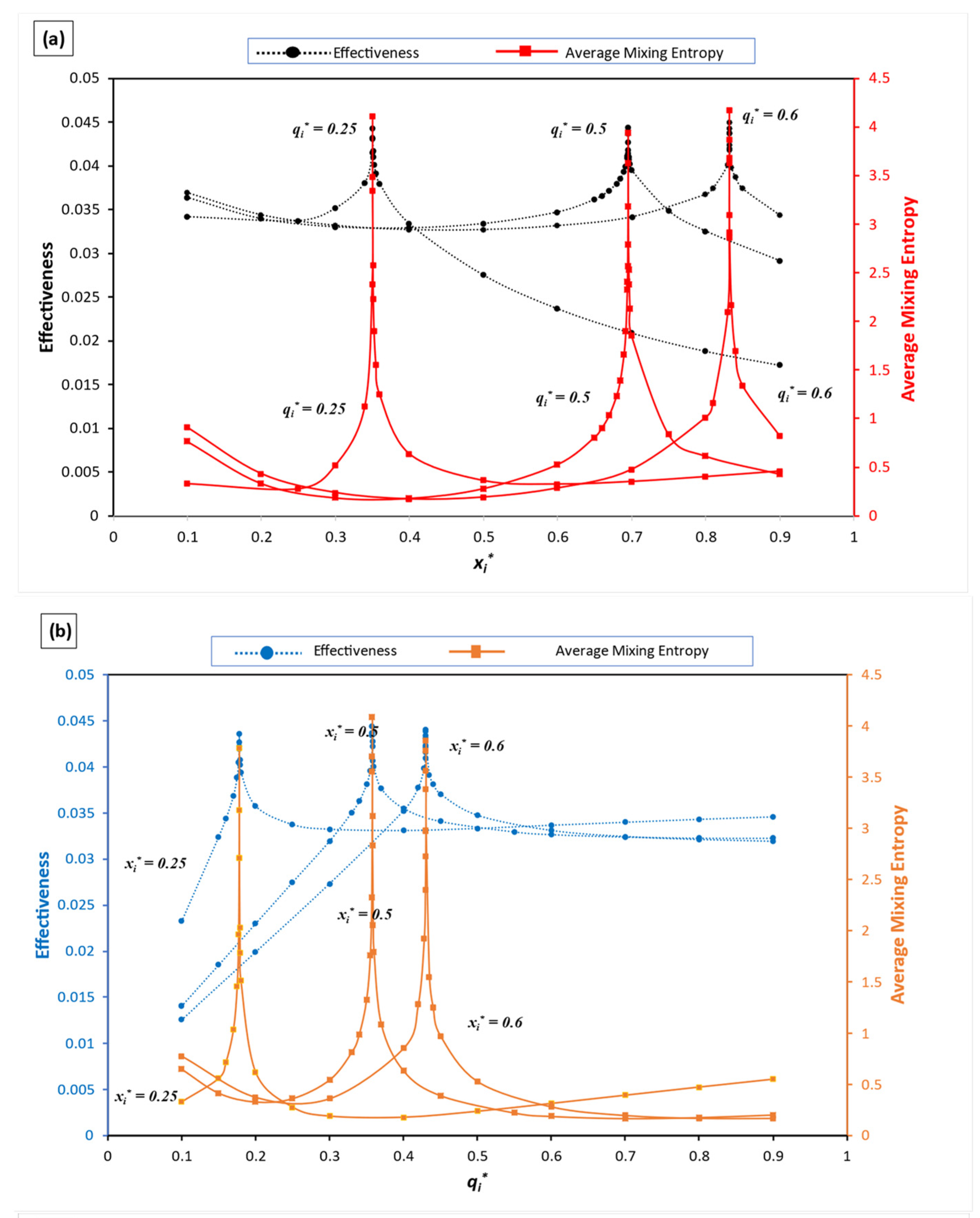
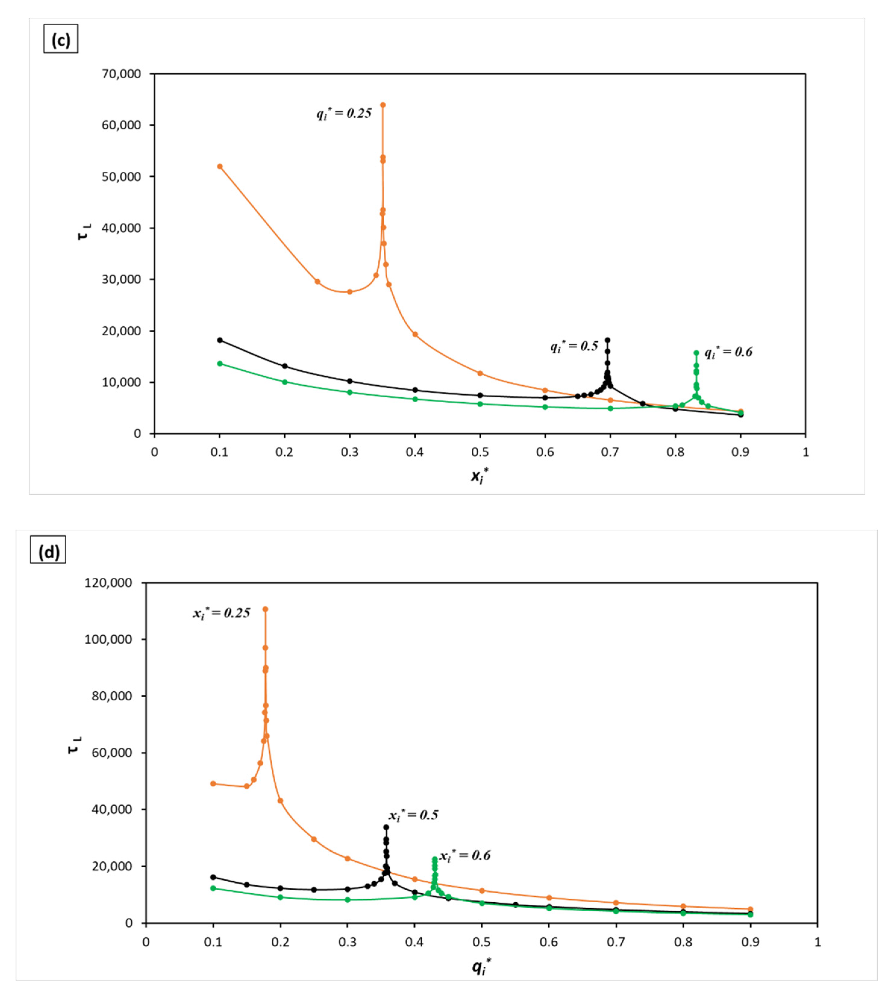
Next, the energy of the system is held constant, while the ratio of the initial mechanical to electrical energy is varied. Figure 5 shows the results for varying $x_i^{*}$ and $q_i^{*}$, or, in other words, varying the ratio of the mechanical energy to the total energy, with a constant total energy of the system of 0.4875. The same trend of mixing entropy and effectiveness is observed as in the previous section. In this case, the peak in effectiveness and mixing entropy occurs at a ratio of mechanical to total energy of 67%. These results further strengthen the conclusion that there is a pair of optimum $x_i^{*}$ and $q_i^{*}$ values for which the mixing entropy and the energy exchange is maximized. The existence of these pairs could be explained by considering the effect an increase in the initial charge has on a mechanical oscillator when the system energy is fixed. The energy transfer between the two domains is directly proportional with $q^{}{*}^2$, thus $q_i^{*}{}^2$, as seen in Equation (13). Thus, increasing the initial charge is expected to increase the net energy transfer. However, the net energy transfer is also proportional with the displacement of the variable capacitor, or more precisely $\left(1-x^{*}\right)$. A charge too large will produce a strong electrostatic attraction force that will increase the oscillation amplitude of the mass, stretching the spring. Thus, a higher portion of the system initial energy will remain in the mechanical system.

It is of interest to note that the peak in effectiveness seen in Figure 5, along with all of the other effectiveness peaks displayed in Figure 3a,b, occur at a ratio of initial mechanical to total energy of 67%. For all peaks shown in Figure 3, the effectiveness value is approximately 0.044 or 4.4%. The slight variations seen between the peaks are due to the high sensitivity of the peak value to small changes in the $x_i^{*}$ and $q_i^{*}$. The mixing entropy with a sharper peak is more sensitive than effectiveness to these variations. This suggests that effectiveness is independent of the initial conditions and is set by the system’s parameters.

3.3. Varying $C_1$ and $C_3$

The solutions of Equations (8) and (9), $q^{*}$ and $x^{*}$, depend on $C_1$, $C_2$, and $C_3$, and initial conditions $q_i^{*}$ and $x_i^{*}$. At resonance $C_2+C_3=1$, and $C_2$, the third term appearing in Equation (9), is dependent on $C_3$. Thus, at resonance, $q^{*}$ and $x^{*}$ solutions depend on $C_1$, $C_3$, and the initial conditions $q_i^{*}$ and $x_i^{*}$. The analysis in previous section has shown that effectiveness and mixing entropy are independent of initial conditions. Consequently, the remaining parameters that could influence the effectiveness and mixing entropy are $C_1$ and $C_3$, and their effect is investigated next. However, the entropy formulation employed in this study requires weak coupling, and both $C_1$ and $C_3$ must be equal or less than 0.1 to meet this condition. Because of this restriction, only one more value, 0.03, was added for both $C_1$ and $C_3$ in addition to 0.1, and all possible ($C_1$, $C_3$) combinations were investigated. Specifically, for each ($C_1$, $C_3$) pair, multiple simulations were run varying $E_{1,i}^{*}/E^{*}$ to determine the maximum effectiveness and mixing entropy values.

The peaks in effectiveness and mixing entropy value for each ($C_1$, $C_3$) are shown in

Table 1. Mixing entropy and effectiveness for different ($C_1$, $C_3$ ) value pairs.

${\mathit{C}}_1$	${\mathit{C}}_3$	Average Mixing Entropy	Effectiveness
0.03	0.03	4.359	0.013
0.03	0.1	4.325	0.044
0.1	0.03	4.966	0.013
0.1	0.1	4.174	0.044

. It should be noted that in all cases, the peak also occurred at $E_{1,i}^{*}/E^{*}=0.67$. From Table 1, it can also be seen that effectiveness depends strongly on $C_3$. For instance, looking at a constant $C_1$ value of 0.03 and following the increase in $C_3$ from 0.03 to 0.1, the effectiveness increases from 0.013 to 0.044, while mixing entropy changes little. Almost identical changes in effectiveness and mixing entropy are seen when $C_1$ is kept at 0.1 and $C_3$ is again increased from 0.03 to 0.1. On the other hand, when $C_3$ is fixed at 0.03 and $C_1$ is increased from 0.03 to 0.1, the effectiveness and mixing entropy remain almost unchanged. The same trend is observed when $C_3$ is fixed at 0.1 and $C_1$ increases from 0.03 to 0.1, although the effectiveness value is higher due to the higher $C_3$. Thus, it can be concluded that in the small interval considered here for $C_1$ and $C_3$ (0.03–0.1), only changing $C_3$ has a noticeable effect on effectiveness, while the effect of both $C_1$ and $C_3$ on the mixing entropy is unremarkable. In conclusion, the squared ratio of the natural frequency of the nominal coupling capacitor to the natural frequency of the mechanical system appears to be a key factor in the effectiveness of energy transfer between the two sub-systems.

4. Conclusions

This paper explores the concept of mixing entropy, borrowed from statistical mechanics, to characterize coupled non-dissipative mechanical–electrical oscillators. Mixing entropy allows for an easier energy flow between the two systems. The trends in average mixing entropy and the effectiveness of energy transfer between the two energy domains is investigated for the case where the natural frequency of the mechanical oscillator is set to be identical to that of the electrical oscillator. For this condition, it is found that the mixing entropy can predict the peak in effectiveness of the energy transfer between the two domains. The results of this study also suggest that the effectiveness of the energy transfer in these conservatively coupled mechanical oscillators can be more effectively enhanced by increasing the initial mechanical energy, rather than the initial electrical energy of the system. Most importantly, for the cases studied here, the maximum mixing entropy and effectiveness values, indicating the maximum energy transfer between the two domains, always occur when the ratio of the initial mechanical domain energy to the total energy of the system is 67%. Furthermore, the effectiveness is sensitive to the squared ratio of the natural frequency of the nominal coupling capacitor to the natural frequency of the mechanical system. A system operating at maximum effectiveness, however, shows the slowest rate of energy transfer from the mechanical to electrical domain. The studies presented here have implications and pave the way for a better understanding of the critical parameters that control the power flow in coupled mechanical–electrical oscillators and their energy conversion limits.

References

1. Xidasiot.com. 2022. Available online: https://xidasiot.com/power/veg (accessed on 23 July 2022).
2. Enoceoan. Available online: https://www.enocean.com/ (accessed on 23 July 2022).
3. Mide. Available online: http://www.mide.com/ (accessed on 23 July 2022).
4. Piezo. Available online: https://www.piezo.com/ (accessed on 23 July 2022).
5. Mitcheson, P.D.; Yeatman, E.M.; Rao, G.K.; Holmes, A.S.; Green, T.C. Energy harvesting from human and machine motion for wireless electronic devices. Proc. IEEE 2008, 96, 1457–1486. [Google Scholar] [CrossRef]
6. Oxaal, J.; Hella, M.; Borca-Tasciuc, D.A. Electrostatic MEMS vibration energy harvester for HVAC applications with impact-based frequency up-conversion. J. Micromech. Microeng. 2016, 26, 124012. [Google Scholar] [CrossRef]
7. Lu, Y.; Juillard, J.; Cottone, F.; Galayko, D.; Basset, P. An impact-coupled MEMS electrostatic kinetic energy harvester and its predictive model taking nonlinear air damping effect into account. J. Microelectromech. Syst. 2018, 27, 1041–1053. [Google Scholar] [CrossRef]
8. Li, J.; Tichy, J.; Borca-Tasciuc, D.A. A predictive model for electrostatic energy harvesters with impact-based frequency up-conversion. J. Micromech. Microeng. 2020, 30, 125012. [Google Scholar] [CrossRef]
9. Li, J.; Tong, X.; Oxaal, J.; Liu, Z.; Hella, M.; Borca-Tasciuc, D.A. Investigation of parallel-connected MEMS electrostatic energy harvesters for enhancing output power over a wide frequency range. J. Micromech. Microeng. 2019, 29, 094001. [Google Scholar] [CrossRef]
10. Tvedt, L.G.W.; Nguyen, D.S.; Halvorsen, E. Nonlinear behavior of an electrostatic energy harvester under wide-and narrowband excitation. J. Microelectromech. Syst. 2010, 19, 305–316. [Google Scholar] [CrossRef]
11. Lu, Y.; Cottone, F.; Boisseau, S.; Marty, F.; Galayko, D.; Basset, P. A nonlinear MEMS electrostatic kinetic energy harvester for human-powered biomedical devices. Appl. Phys. Lett. 2015, 107, 253902. [Google Scholar] [CrossRef]
12. Honma, H.; Mitsuya, H.; Hashiguchi, G.; Fujita, H.; Toshiyoshi, H. Improvement of energy conversion effectiveness and maximum output power of electrostatic induction-type MEMS energy harvesters by using symmetric comb-electrode structures. J. Micromech. Microeng. 2018, 28, 064005. [Google Scholar] [CrossRef]
13. Roundy, S. On the effectiveness of vibration-based energy harvesting. J. Intell. Mater. Syst. Struct. 2005, 16, 809–823. [Google Scholar] [CrossRef]
14. Halvorsen, E. Electrostatic energy harvesters and fundamental limits to power. J. Phys. Conf. Ser. 2018, 1052, 012004. [Google Scholar] [CrossRef]
15. Toshiyoshi, H.; Ju, S.; Honma, H.; Ji, C.H.; Fujita, H. MEMS vibrational energy harvesters. Sci. Technol. Adv. Mater. 2019, 20, 124–143. [Google Scholar] [CrossRef] [PubMed]
16. Martinelli, M. Entropy, carnot cycle, and information theory. Entropy 2019, 21, 3. [Google Scholar] [CrossRef]
17. Tavares, J.M.; Patricio, P. Maximum thermodynamic power coefficient of a wind turbine. Wind Energy 2020, 23, 1077–1084. [Google Scholar] [CrossRef]
18. Kostic, M.M. Revisiting the second law of energy degradation and entropy generation: From Sadi Carnot’s ingenious reasoning to holistic generalization. AIP Conf. Proc. 2011, 1411, 327–350. [Google Scholar]
19. Haddad, W.M. Thermodynamics: The unique universal science. Entropy 2017, 19, 621. [Google Scholar] [CrossRef]
20. Dicer, I.; Cengel, Y.A. Energy, Entropy and Exergy Concepts and Their Roles in Thermal Engineering. Entropy 2001, 3, 116–149. [Google Scholar] [CrossRef]
21. Wu, J.; Guo, Z.Y. Entropy and its correlations with other related quantities. Entropy 2014, 16, 1089–1100. [Google Scholar] [CrossRef]
22. Zorich, V.A. Entropy in thermodynamics and information theory. Probl. Inf. Transm. 2022, 58, 3–11. [Google Scholar] [CrossRef]
23. Sunar, M.; Sahin, A.Z.; Yilbas, B.S. Entropy generation rate in a mechanical system subjected to a damped oscillation. Int. J. Exergy 2015, 17, 401–411. [Google Scholar] [CrossRef]
24. Le Bot, A. Entropy in statistical energy analysis. J. Acoust. Soc. Am. 2009, 125, 1473–1478. [Google Scholar] [CrossRef]
25. Prajwal, K.T.; Manickavasagam, K.; Suresh, R. A review on vibration energy harvesting technologies: Analysis and technologies. Eur. Phys. J. Spec. Top. 2022, 231, 1359–1371. [Google Scholar] [CrossRef]
26. Lensvelt, R.; Fey, R.H.B.; Mestrom, R.M.C.; Nijmeijer, H. Design and numerical analysis of an electrostatic energy harvester with impact for frequency up-conversion. J. Comput. Nonlinear Dyn. 2020, 15, 1–8. [Google Scholar] [CrossRef]
27. Yamane, D.; Tamura, K.; Nota, K.; Iwakawa, R.; Lo, C.-Y.; Miwa, K.; Ono, S. Contactless Electrostatic Vibration Energy Harvesting Using Electric Double Layer Electrets. Sensors Mater. 2022, 34, 1869. [Google Scholar] [CrossRef]
28. Mahmud, M.A.P.; Bazaz, S.R.; Dabiri, S.; Mehrizi, A.A.; Asadnia, M.; Warkiani, M.E.; Wang, Z.L. Advances in MEMS and Microfluidics-Based Energy Harvesting Technologies. Adv. Mater. Technol. 2022, 2101347, 1–30. [Google Scholar] [CrossRef]
29. Lyon, R.H.; Maidanik, G. Power Flow between Linearly Coupled Oscillators. J. Acoust. Soc. Am. 1962, 34, 623–639. [Google Scholar] [CrossRef]
30. Carcaterra, A. An entropy formulation for the analysis of energy flow between mechanical resonators. Mech. Syst. Signal. Process. 2002, 16, 905–920. [Google Scholar] [CrossRef]
31. Le Bot, A. Entropy in sound and vibration: Towards a new paradigm. Proc. R. Soc. A Math. Phys. Eng. Sci. 2017, 473, 20160602. [Google Scholar] [CrossRef]
32. Tufano, D.; Sotoudeh, Z. Exploring the entropy concept for coupled oscillators. Int. J. Eng. Sci. 2017, 112, 18–31. [Google Scholar] [CrossRef]
33. Tufano, D.A.; Sotoudeh, Z. Entropy for Strongly Coupled Oscillators. J. Vib. Acoust. Trans. ASME 2018, 140, 1–8. [Google Scholar] [CrossRef]
34. Berdichevsky, V. Thermodynamics of Chaos and Order; Addison Wesley Longman Limited: Harlow, UK, 1997. [Google Scholar]
Figure 1. The coupled mechanical–electrical oscillators.
Energies 15 06105 g001
Figure 2. Normalized electrical ( E 2 * ) and mechanical ( E 1 * ) energies (top), and instantaneous mixing entropy (bottom) as a function of the nondimensional time t*. Insets show the local high frequency vibrations.
Energies 15 06105 g002
Figure 3. Effectiveness and average mixing entropy as a function of increasing x i * (a), and q i * (b). Corresponding period of the large-scale oscillation, τ L (as shown in Figure 2) of energy transfer between the mechanical and electrical domains for increasing x i * (c), and q i * (d).
Energies 15 06105 g003aEnergies 15 06105 g003b
Figure 4. Moving average of the normalized electrical ( E 2 * ) and mechanical ( E 1 * ) energies (top), and moving average of the instantaneous mixing entropy (bottom) as a function of the nondimensional time t* for x i *   = 0.833206, and q i *   = 0.6, which give peak conditions in effectiveness and τ L .
Energies 15 06105 g004
Figure 5. Effectiveness and averaged mixing entropy as a function of the fraction of the initial mechanical energy to the total energy.
Energies 15 06105 g005