1. Introduction
Since the United Nations proposed an annual meeting between representatives of the 190 nations to discuss climate change and address carbon dioxide (CO2) emissions from fossil fuels, countries have become more engaged in addressing the subject seriously. Researchers have proposed alternative energy sources such as using the sun, the wind, nuclear energy, or harvesting geothermal energy. Nevertheless, despite recent implementations sanctioned by various governments, CO2 emissions continue rising, and it took a global pandemic to change the expected 1% growth for CO2 emissions. However, activities seem to be returning to normal, heightening the need for cleaner energy and making reducing unnecessary energy consumption more urgent.
Moreover, the number of household appliances has kept increasing since the 1960s, when the television, refrigerator, and washing machine were the main elements in a home. Modern households currently contain many more energy-consuming appliances, depending on the number of persons in the household. Research indicates an average of 10 or more appliances inside a modern household with only one person living inside [
1]. Therefore, it is imperative to evaluate which are the ones that consume the most energy and address their use to help the user operate them in the most energy-efficient manner.
One of the most energy-consuming appliances is the Heating and Ventilation Air-Conditioning System (HVAC). Research indicates that more than 60% of homes have these systems, and more than 85% have thermostats in their home [
2]. Therefore, it is vital to avoid the unnecessary use of these systems to save energy. The method developed to approach an efficient use of such appliances is the concept of thermal comfort. The American Society of Heating, Refrigerating and Air-Conditioning Engineers (ASHRAE) defines Thermal Comfort as “the condition of the mind in which satisfaction is expressed with the thermal environment” [
3]. Moreover, it takes into account six different factors to calculate thermal comfort: air temperature, radiant temperature, air speed, humidity, metabolic rate, and clothing insulation. Medina et al. [
4] proposed to analyze clothing insulation to learn about householder garments’ preferences and analyze their thermal comfort to send messages to interactive interfaces that suggest the householder use warmer or cooler garments to increase, maintain, or decrease the set point to promote energy reduction. However, this proposal lacked implementation on an embedded system. It just proposed an interactive interface in the MATLAB/Simulink R2021a environment.
Research about implemented interactive interfaces to engage householders in game-like activities that help them reduce energy have been proposed [
2,
5,
6,
7,
8]. However, these proposals consider static activities and garments. The PMV/PPD and adaptive models calculate thermal comfort depending on several factors, considering the metabolic rate and clothing insulation in both models. Activity affects the metabolic rate and therefore affects the amount of heat the body produces. Moreover, different clothing garments affect the heat transfer between the user and the ambient air, representing a clothing insulation value. Some studies calculate the metabolic rate using thermal cameras or Kinect [
9,
10,
11,
12,
13]. Regarding the clothing insulation classifier, Liu et al. [
14] proposed using a thermal camera to dynamically estimate each person’s clothing insulation and metabolic rate. Choi et al. [
15] classified five classes of garments and proposed a method for estimating clothing insulation using deep-learning-based vision recognition by classifying five classes of garments. Medina et al. [
4] classified eight classes of garments using the YOLOv3 model to propose its implementation in a connected mock-up thermostat.
1.1. One-Stage Object Detector and Classifiers
Object detection and classification have two main research lines: one-stage and two-stage algorithms. Two-stage algorithms detect objects and delimit them with bounding boxes; then, a second stage classifies the objects detected inside that image and better delimits the detected object; an example is the Mask R-CNN [
16]. On the other hand, the one-stage detectors provide object detection and classification in a single pass; therefore, they are faster but less accurate than the two-stage algorithms. Hence, the one-stage methods are faster and require less processing power, making them suitable for a small system such as an embedded system.
Inside the one-stage classifiers, two main algorithms are presented as solutions: the Single Shot Detector (SSD) [
17] and the You Only Look Once (YOLO) [
18] algorithms. SSD is faster but less accurate, according to the last comparisons by YOLO authors [
19]. YOLO has been integrating and outputting official variations to its algorithm more often, improving its performance.
YOLO is one of the most popular object detector algorithms, and it was created in 2016 by Redmon et al. [
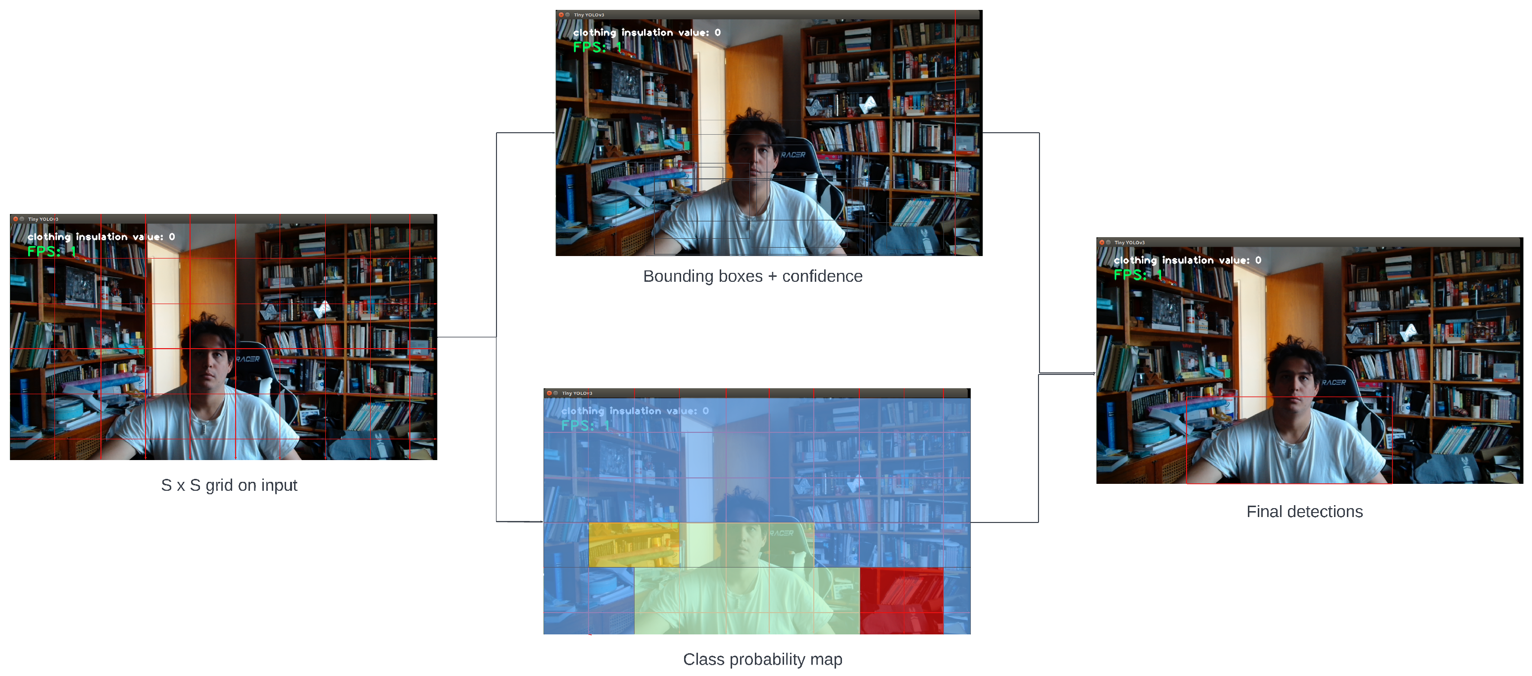
18]. The authors’ main goal was to create an accurate deep learning algorithm that could be faster than the existing algorithms. They proposed to look at the entire image and produce predictions for bounding boxes as well as class probabilities for those boxes.
Figure 1 exemplifies this concept by using a grid system to look into each cell in the grid to produce the probabilities for the bounding boxes and classes. The different algorithms of YOLO change because different authors propose new versions of YOLO. Thus, a general review of their architectures and how they have evolved is presented.
1.1.1. YOLOv3 and Tiny YOLOv3
The YOLOv3 model was implemented in a Linux environment, allowing training with custom datasets. Moreover, this model includes the weights of pre-trained algorithms using the COCO dataset [
20] to perform transfer learning or to train existing models.
The TinyYOLOv3 is a smaller version of the YOLOv3 with a minor architecture that make its implementation easy in a more computationally restricted system [
19].
The main difference between the full YOLOv3 model and the Tiny YOLOv3 model is that the full model does not use pooling layers, and the Tiny YOLOv3 model does. Tiny YOLOv3 only performs recognition at two different sizes instead of three; however, due to the algorithm’s size, it is much faster than the full model.
Figure 2 pictures the YOLOv3 Model, and
Table 1 depicts the Tiny YOLOv3 architecture.
1.1.2. YOLOv4 and Tiny YOLOv4
Since the principal author of the original YOLO algorithm decided to stop the research on computer vision algorithms, some authors decided to take the algorithm and try to keep improving it since it was a high-speed algorithm. However, the accuracy was still below the two-stage algorithms. One of the models proposed is YOLOv4, developed by Bochovskiy et al. [
21].
Hence, YOLOv4 has a variation of the DarkNet-53 used as backbone called CSPDarkNet53. This backbone was chosen after comparing the most common backbones, such as CSPDarkNet53 and CSPResNext50. In addition, the author followed Redmon’s footsteps and provided the Tiny YOLOv4. There is no current comparison between the YOLOv4 and the Tiny YOLOv4.
Consequently,
Figure 3 shows both algorithms.
Figure 3a shows that YOLOv4 uses pooling layers but only for the newly added Spatial Pyramid Pooling (SPP) to improve the detection method by not modifying the input image size. The DarkNet53 backbone remains free of pooling layers.
Figure 3b shows that the Tiny YOLOv4 continues to work with pooling layers; however, this newer version skips connections to try and help the algorithm retain more feature information.
1.1.3. YOLOv5
Jocher et al. [
22,
23] proposed the recent version of the YOLO algorithm, the YOLOv5. This algorithm is for public use because they changed the Linux environment requirement into an open source approach. They implemented YOLOv5 in Python through PyTorch rather than DarkNet. Therefore, they allowed Windows users to create virtual environments and to train it locally, for instance, in Anaconda, instead of Google Colab.
These authors proposed five models, from smallest to largest: YOLOv5n, YOLOv5s, YOLOv5m, YOLOv5l, and YOLOv5x. Nevertheless, due to the lack of a scientific paper, there is no apparent difference in the models; Azam et al. [
24] indicated that the difference relied on the scaling multipliers of the width and depth of the network. Therefore, the architecture is the same but the size changes. Thus, YOLOv5 algorithms enable more accessible training in computationally restricted environments than the previous versions of YOLO (See
Figure 4).
1.2. Embedded Systems
An embedded system has minimum hardware requirements based on a microprocessor designed for a specific purpose. Thus, most times it is custom-made. There are some development boards to perform tests before assembling the custom board, and these systems test simple functionalities and different sensor and actuator capabilities. Therefore, the main benefit of these boards is that they come with some Light Emitting Diodes (LEDs) to simulate the actuators’ activation and some push buttons to simulate the inputs from a sensor. Moreover, compatible extension boards have been developed for different sensors or actuators, such as cameras, motor drivers, and wireless communications. Even though the development boards are not fully customized for a certain solution, they are microprocessor-based and practically next to the final custom embedded system solution. Hence, they are considered embedded systems.
Figure 5 shows the embedded systems used for this research.
Figure 5a depicts the Raspberry Pi 4 board, and
Figure 5b portrays the Jetson Nano board.
Raspberry Pi [
25] focuses on offering a more robust development board while competing with the most expensive Arduino boards on the market. This development board does not have its IDE. However, the developers advertised it as a mini-computer, so instead, they developed its operating system called Raspbian. This operating system uses free distribution operating system called Debian, which is built on top of a Linux kernel [
26]. Raspberry Pi 4 Model B is the most recent board; it has a Broadcom BCM2711B0 quad-core Cortex-A72 processor running at 1.5 GHz with a VideoCore VI 500 MHz GPU with 4 GB LPDDR4-3200 memory.
On the other hand, the company NVIDIA proposed their line of embedded system boards called Jetson. They are oriented toward Artificial Intelligence (AI) solutions. One of these boards is the Jetson Nano [
27]; this board has a Quad-core ARM Cortex-A57 MPCore processor with an NVIDIA Maxwell with 128 CUDA cores GPU a 4 GB 64-bit LPDDR4-1600 memory.
1.3. Computer Vision in Embedded Systems
Some researchers have worked with embedded systems to implement computer vision algorithms for different purposes. According to Stankovic [
28], there have been three major trends involving embedded systems and real-time solutions:
The development of the architecture used in the embedded systems has been growing fast and has achieved real-time constraints.
Achieve hard real-time results where missing a deadline means the failure of the solution.
Soft real-time solutions: If there is some failure in the real-time part of the solution, it is possible to manage and provide results avoiding the system’s failure.
This paper focuses on soft real-time solutions. Jin et al. [
29] modified the YOLOv3 algorithm to detect and classify pedestrians using a Jetson TX2 embedded system. With their customized architecture, the authors reached 9-10 frames per second (FPS) on the system. Chen et al. [
30] customized another version of the YOLOv3 to detect cars in the street. They also work around the bit floating point difference for the embedded system to use resources in an embedded system efficiently. Thus, with their custom architecture and bit floating point calculation quantization, they achieved 28 FPS. However, the authors do not specify which embedded system they used for their tests. Therefore, it is feasible to implement solutions for energy savings at home, for instance, in a connected thermostat, to reduce energy consumption at home.
Murty et al. [
31] discussed different algorithms tested with different embedded systems. Unfortunately, the results comparing such systems present older algorithms and only Powerful AI-oriented Boards such as Jetson TX2. Therefore, a new comparison is needed to assess whether existing algorithms can be used for object detection and classification to avoid needing custom-built architectures, hardware enhancers, or expensive AI-oriented embedded systems.
Taylor et al. [
32] identified the best algorithm depending on the image input on the Jetson TX2 and compared the models with the Inception and ResNet algorithms. Dedeoglu et al. [
33] proposed special computer vision libraries for embedded systems. Medina et al. [
4] suggested that YOLO algorithms classified better clothing garments in real-time than the ResNet18, Inceptionv4, and VGG16 architectures. Therefore, this paper focuses on determining the best YOLO architecture with the fastest response in an embedded system. Thus, the computer vision system deploys the algorithms and analyzes the experiments to obtain enough information to implement the clothing classification as a companion system in connected thermostats.
Figure 6 proposes how the connected thermostat interacts with the real-time clothing classifier and the end-user for reducing energy consumption at home according with [
4,
34,
35]. The connected thermostat uses the real-time clothing classifier to determine the thermal comfort zone. Consequently, the temperature set point is adjusted to save energy. A message is displayed in the connected thermostat asking the householder to accept this new set point value. This paper focuses on the real-time clothing classifier as it is the main component in the proposed structure. This is carried out by determining which YOLO algorithm best fits the embedded system to provide information in real time. As a result, we obtain the best solution between the tested options, concluding that it is feasible to deploy this in a real environment.
The remainder of this paper is as follows.
Section 2 describes the methodology used for the clothing classifier and the embedded systems. Consequently,
Section 3 describes and compares the results of each YOLO algorithm with each embedded system.
Section 4 describes the scope of the research and discusses the advantages and disadvantages of each comparison. Finally, conclusions and suggestions for future work are presented in
Section 5.
2. Methodology
Figure 7 presents the flow diagram of the real-time clothing classifier in which the programmable code loads the corresponding algorithm weights in order to just dedicate itself to the classification. then the whole loop starts, and the video capture commences to start obtaining the information from the camera, the time stamp is taken for later comparison, and the classification information such as bounding boxes, class, and confidence values are produced. Then the new time stamp is taken to obtain the difference in time and obtain the FPS with an equation presented later. This process repeats itself until the user stops the program and resets and restarts the variables.
This research compares already existing algorithms and applies them to embedded systems [
19,
21]. This comparison helps those who look for an algorithm to be implemented in an embedded system and even sees if the existing algorithms may help solve their problems. Nevertheless, many possibilities and many variables may affect the results presented in this paper. For example, hardware enhancers may increase the amount of FPS obtained, and code optimization or a network trained with different settings or datasets may improve or worsen its accuracy values.
Therefore, this section compares YOLO v3 with the Tiny YOLOv3, YOLOv4 with the Tiny YOLOv4, and three different sizes of YOLOv5 to determine which of these architectures has the fastest response in the implementation of the embedded system without losing accuracy. The accuracy test was performed multiple times in the same room, with variations on clothing garments of the same class, one hardware system after the other, to avoid significant lighting differences between classifications. Thus, the algorithms were tested on the computer and in the Raspberry Pi 4 and Jeston Nano.
One-stage classifiers were chosen to compare different algorithms for object detection and classification because they are faster and have fewer parameters to train, so the most common one-stage algorithms are Tiny YOLOv3 [
19], YOLOv3 [
19], YOLOv4 [
21], Tiny YOLOv4 [
21], YOLOv5n [
22], YOLOv5s [
22], and YOLOv5m [
22], among other algorithms. Although the literature review showed little to few implementations of these algorithms in embedded systems and better customized the YOLO versions [
29,
30,
36,
37,
38], this paper prefers using algorithms and training datasets for clothing garments to modifying them because it is easier for other researchers to replicate this research methodology than adapt algorithms.
For this custom dataset for clothing recognition, images were taken from the Internet and labeled.
Figure 8 shows an example of this classification. Since the number of training images is a factor to be considered when choosing the hypertraining parameters, 2000 images were selected where there were multiple persons or just a single person in a frame and with different backgrounds. However, these images have a small dataset, so image transformations such as flipping, contrast changes, color changes, blurring, and other transformations were performed on all images to increase the training dataset and obtain a final 15,000-image dataset.
Figure 9 shows an example of this type of transformation. These transformations also address the difference in camera resolution and lighting settings so that when implemented, cameras with less resolution or darker settings do not struggle too much performing the classifications, as well as removing the orientation variable out of the equation by using the flipping transformations.
The algorithms are trained using 16,000 epochs ashyperparameters, with alearning rate of 0.01, astheauthors recommend forcustom training, and using theAdam Optimizer to have amore objective comparison. Then, these algorithms are implemented inacomputer that has aGeForce RTX 2080 Ti GPU with 11 GB GGDR6 RAM and anAMD Ryzen 3950 12 core 3.5 GHz processor with 64 GB ofRAM memory (PC). Thetrained models run using OpenCV toaccess thecamera and theresulting weights for each model toobtain theprediction inareal-time implementation and measure accuracy and Frames Per Second (FPS).
The YOLOv3, Tiny YOLOv3, and Tiny YOLOv4 algorithms were trained using Google Colab due to the fact that there was no access to a Linux environment, and Colab allows us to use the Darknet framework these algorithms have. So, in order to keep the comparison as fair as possible (since the author of the YOLOv4 algorithm has stated that the comparison presented by the author of the YOLOv5 model was using the version he implemented with PyTorch framework and not the native Darknet framework which affects the algorithms results) the authors selected the one using the Darknet framework.
The training time for the YOLOv3 algorithm was around 300 h (an approximate time is used since Colab allows access to Cloud GPU computing for 4 h a day, and you cannot choose the GPU, so it may change from day to day), the Tiny YOLOv3 took around 120 h, and the Tiny YOLOv4 took around 90 h.
YOLOv5 implemented an early stop in the training code, so if the Mean Average Precision (mAP) does not change after 100 epochs, the training stops; therefore, training for the YOLOv5 algorithms was shorter and only reached an average of 350 epochs. There is the option to change this parameter. However, after changing it to have an early stop after 500 epochs, the results of the mAP were the same for the trained algorithm, and since the point is to train all the algorithms in the same manner, no more tuning to the parameters was performed. Before the comparison, a quick test was made to see if the YOLOv5 algorithms managed to detect and classify objects with such short training, and since they did, the comparison continued as planned. The training times for the YOLOv5 algorithms were all around the 3 h mark.
The comparison focuses on two metrics: accuracy and FPS. The accuracy was measured using an object detector threshold of 70 to avoid miss-classifications of detected objects that are not within the desired results. Therefore, the accuracy uses the percentage of different clothing garments recognized with different real-time tests. It is performed with a Logitech HD Pro C920 Web Camera connected to the different systems in the same room at different times during the day to leave out possible bias due to different lighting settings caused by the difference in day times.
The FPS were measured using the time library available in Python and is calculated measuring the time stamp of the model when it loads the image and after then applying Equation (
1). Since the program loads the image again, a measurement of frames per second, analysis can be obtained.
Three different clothing garments are chosen for eight classes in order to have some different colors and textures to present different possibilities, such as the examples shown in
Figure 10.
Table 2 depicts the classes analyzed. Each class was tested for every hardware system in a consecutive manner to avoid having too much difference in light settings due to the difference in day times.
3. Results
Figure 11 shows the results in the PC.
Figure 11 shows the Jetson Nano results for a seated individual with a white T-shirt and with the display turned on.
Figure 12 depicts the Raspberry Pi 4 results with the display turned on, too. These figures show how the system worked in each one. Although the computer is above the hardware capabilities of an average personal computer (PC), it is still not good enough for an AI-oriented computer that requires at least a Titan X or Tesla V100 GPU.
Table 3 and
Table 4 present the information on both embedded systems but with the display turned off. Thus, the results were printed on the console. The columns correspond to the model the results refer to, the Highest FPS value the model reached, the Average FPS value the model had in 10 seconds run time, the accuracy of the model recognizing different clothing garments, and the average class probability the model produced for a white shirt test.
After observing the results with the display active, the clear difference between the computer and both embedded systems is noticeable. All models suffer a loss of about 80% in the FPS metric they could produce. However, Raspberry Pi 4 seems to perform better than the Jetson Nano, which was unexpected. A clear difference can be seen comparing
Figure 12 and
Figure 13, where the full YOLOv3 model crashed when running in the Jetson Nano (that is why there is a grayscale image), and even though it had its fair share of problems, it does not crash in the Raspberry Pi 4.
In addition, comparing the tests performed with the display turned off with the displays turned on, the FPS metric does not differ by a significant amount in the Raspberry Pi 4, and even though in the Jetson Nano, it helped the bigger models such as YOLOv3, YOLOv5s, and YOLOv5m the difference was not that great. The only difference made was to turn off the display, so a code optimization to eliminate unnecessary things may increase the models’ performance. However, the display alone was not responsible for downgrading the smaller models’ performance by comparing the FPS values in
Figure 12 and
Figure 13 with those in
Table 3 and
Table 4.
4. Discussion
Both PMV/PPD and adaptive methods share the met and clothes factors. However, this proposal considers the activity factor static, whereas the clothing insulation is dynamic. In Medina et al. [
4], the authors had previously simulated the clothing insulation using MATLAB/Simulink. They found that the HVAC energy consumption decreased from 18% to 47% by providing feedback about the clothing insulation. Thus, succeeding in those simulated reductions, this paper focuses on implementing this solution in embedded systems. Therefore, future work includes deploying this embedded system into a connected thermostat and implementing it in a physical space to analyze the impact of reducing energy while maintaining thermal comfort.
These FPS results are similar to those presented in [
39]. Although 3 to 7 FPS is a significant difference, it would not be enough for implementation in an autonomous car. It is not necessary to achieve these FPS for calculating the clothing insulation value. Thermal comfort models usually consider the clothing for larger periods of time, for instance, during a day, week, or month. Hence, the FPS achieved in this proposal helps provide new ways of saving energy by taking advantage of current technology and using deep learning computer vision algorithms in embedded systems.
In addition, the accuracy results showed little change between all hardware systems. Although the models implemented in the Raspberry Pi 4 showed better performance compared to the models implemented in the Jetson Nano by about a 3% difference, the number of tests is not enough to conclude that the hardware system affects the accuracy of the model significantly. Recognizing one of the three chosen clothing garments for each class would increase the accuracy value by almost 5%. Moreover, comparing each model with the PC results, the difference is practically non-existent, only 1% for each model between hardware implementations and the PC results.
5. Conclusions
This paper proposes a real-time clothing classifier to be implemented in a connected thermostat that does not require more than seven or eight FPS. Six YOLO models were successfully implemented and evaluated in a Raspberry Pi 4 and the Jetson Nano. A complete analysis of these embedded systems was conducted.
The results show that embedded systems and existing algorithms achieve soft real-time acquisition. In this application, one or two FPS is sufficient to classify clothing. The speed and accuracy of algorithms such as Tiny YOLOv4 and YOLOv5n are enough to be considered a good alternative in this proposal.
YOLOv3 is discarded from this application because even though it had one of the best accuracy results, the processing speed required to obtain classifications is not fast enough without a hardware enhancer. It crashed on the Jetson Nano and ran very slowly on the Raspberry Pi 4. For the Tiny YOLOv3 model, even though it is the fastest model since it achieved FPS values that doubled the FPS of the rest of the algorithms, it lacks accuracy since it does not deliver almost any classifications. Therefore, a more robust training dataset is sufficient to fix this problem. As for the YOLOv5 models, choosing which one is the best for any situation would be better considering that it is the same base architecture, and only the depth changes with each version. However, for embedded systems, the best is YOLOv5n since the accuracy results do not change much, but the FPS is higher on the YOLOv5n algorithm.
The option for choosing a model between Tiny YOLOv4 and YOLOv5n would be Tiny YOLOv4 because it had fewer missed object detections and showed the same speed and increased accuracy as the YOLOv5n model. Nevertheless, the training time difference between models was vastly different. When Google Colab has used, the Tiny YOLOv4 needed more time to be trained than YOLOv5n. The FPS values were similar and presented the most variations between embedded systems, with almost one FPS difference in the case of Tiny YOLOv4. In addition, the results of both embedded systems showed that these systems have the requirements for running computer vision deep learning algorithms. They present results up to one FPS without any help of hardware enhancers or custom algorithms.


 ,
, 


