Solar Irradiance Ramp Forecasting Based on All-Sky Imagers

Abstract

Solar forecasting constitutes a critical tool for operating, producing and storing generated power from solar farms. In the framework of the International Energy Agency’s Photovoltaic Power Systems Program Task 16, the solar irradiance nowcast algorithms, based on five all-sky imagers (ASIs), are used to investigate the feasibility of ASIs to foresee ramp events. ASIs 1–2 and ASIs 3–5 can capture the true ramp events by 26.0–51.0% and 49.0–92.0% of the cases, respectively. ASIs 1–2 provided the lowest (<10.0%) falsely documented ramp events while ASIs 3–5 recorded false ramp events up to 85.0%. On the other hand, ASIs 3–5 revealed the lowest falsely documented no ramp events (8.0–51.0%). ASIs 1–2 are developed to provide spatial solar irradiance forecasts and have been delimited only to a small area for the purposes of this benchmark, which penalizes these approaches. These findings show that ASI-based nowcasts could be considered as a valuable tool for predicting solar irradiance ramp events for a variety of solar energy technologies. The combination of physical and deep learning-based methods is identified as a potential approach to further improve the ramp event forecasts.

1. Introduction

Solar irradiance constitutes the most abundant renewable energy source available. However, solar resource is highly variable, mainly because of clouds, often leading to abrupt changes in solar power generation. For this reason, solar forecasting is considered a valuable tool for the operation of solar technologies. It can support the solar technologies’ operation and integration by using the incoming solar resource to the fullest and improving grid stability.

In the literature, there is no commonly accepted formal definition of a ramp event (RE). A solar irradiance (or power) RE can be defined as an event with a sudden change in solar irradiance (or power) within a short time interval. In particular, an accurate definition depends on the user and the corresponding application [1]. Simplistically, ramps can be identified by calculating the absolute power difference between the starting and ending point of a timeframe [1,2,3]. However, power changes may occur suddenly and consecutively, and not necessarily between the starting and ending timeframe points. The former issue can be addressed by calculating the difference between the minimum and maximum power values within a pre-defined timeframe [1,2]. Alternatively, power REs can be estimated using the power ramp rate (RR) between the starting and ending points at a specific time interval [2]. Power RR, in particular, is the derivative of power over a time interval. All the mentioned RE-detection definitions rely on the user’s need for setting a threshold limit to discriminate an RE from a no-RE.

Solar power systems have mechanisms in place to handle small amounts of uncertainty and variability; however, emphasis is placed on forecasting extreme events, the so-called solar ramp events. Solar REs can be divided into two main categories: (a) solar irradiance REs and (b) solar power REs [4]. Several studies dedicated to solar RE detection exist in the literature. Regarding solar power REs, Abuella and Chowdhury [5] presented an adjusting approach that combines the forecasts derived from different algorithms using an ensemble technique to calculate the solar power RRs on an hourly basis and based on them to estimate the solar power REs. The same methodology of RE detection is also followed by Kong et al. [6] in terms of power forecasts from multiple deep-learning models coming from measurements derived from all-sky imagers (ASIs). Florita et al. [7] implemented a dynamic programming methodology using the Swinging Door (SD) algorithm [8] to identify solar and wind power REs. SD estimates the REs by applying a piecewise linear approximation consisting of only one tunable parameter ($ϵ$) that defines the magnitude of the ramp. The SD algorithm has also been adopted to define a new ramp metric [9] comparing the extracted slopes from the SD algorithm between the forecasts and the measurements within specific time frames. As a next step, the SD algorithm was optimized [10] and implemented for wind and solar power RE detection [4]. Abuella and Chowdhury [11] also utilized several machine-learning classification algorithms to predict REs using solar power forecasts and weather predictions as model inputs.

Several studies regarding solar irradiance REs exist in the literature. Reno and Stein [12] investigated the correlation between the cloud type derived from satellite images and solar irradiance variation. Chu et al. [13] calculated solar irradiance nowcasts by combining the cloud information from a fisheye dome network camera with neural networks. In order to exclude the impact of diurnal solar variability on RE detection, they predicted the REs at a 10 min time horizon using the ASI-based nowcasted solar irradiances in conjunction with clear-sky measurements. Following Chu et al. [13], Cardas and Alonso-Suárez [14] detected REs using ASIs and different solar irradiance forecasting algorithms. Their findings showed that the forecast’s performance in true RE detection is best for high ramp magnitudes and short forecast lead times. Although the accurate forecasting of the abrupt solar irradiance fluctuations is of great importance, relatively few studies have adequately focused on this scientific area, implying a research gap and the necessity of deeper research in this specific domain.

This study is a step forward in a benchmarking exercise conducted in the framework of the International Energy Agency’s Photovoltaic Power Systems Program (IEA PVPS) Task 16. IEA constitutes an autonomous body under the framework of the Organization for Economic Cooperation and Development. The IEA PVPS’s overreaching goal is to enhance the international collaborative efforts that investigate the key role of photovoltaic solar energy in the transition to sustainable energy systems. The first benchmarking exercise was focused on the state-of-the-art solar irradiance nowcasting derived from a bouquet of ASI-based methodologies [15]. The campaign took place at CIEMAT’s Plataforma Solar de Almería (PSA) in southern Spain, where four different ASI systems were installed and measured from August to November 2019. The validation findings highlighted the quite good performance of ASIs concerning nowcast solar irradiance regardless of the underlying cloud conditions. The principal objective of this second benchmarking exercise is to investigate the feasibility of ASI nowcasts in RE prediction. Section 2 presents a brief description of the applied data and the implemented methodologies. Section 3 describes the methodology of solar irradiance RE detection. Finally, the results and conclusions are presented in Section 4 and Section 5, respectively. Since solar forecasting has become an indispensable aspect of solar power system technologies, the presented study aims to evaluate the ability of ASI nowcasts to become a valuable tool for solar irradiance RE prediction.

2. Forecast Algorithms and Ancillary Measurements

Global horizontal irradiance (GHI) is nowcasted up to 20 min ahead in 1 min temporal resolution by four ASI systems. Within the measurement campaign, 28 days from September to November 2019 at PSA in southern Spain were selected to validate GHI nowcasts, including various atmospheric conditions (e.g., cloud types, total aerosol load, etc.). During the campaign, six main cloud clusters (CCs) were detected using visual inspection, varying from almost clear-sky days (CC: 1) to overcast cloud conditions (4A).

Table 1. Cloud clusters and the corresponding number of available evaluation days.

Acronym	Cloud Types	Dates in 2019
		September	October	November	Total
1	Cloud-free (or almost cloud-free)	24, 29	6, 10, 26, 29	8, 18	8
2L	Scattered/broken cloudiness with Low clouds		8	7	2
2M	Scattered/broken cloudiness with Multiple clouds		12, 23, 30	1, 14, 20, 26	7
2H	Scattered/broken cloudiness with High/Middle clouds		1, 7, 18	6, 19, 28	6
3H	Scattered/broken cloudiness with High/Middle clouds	30	5, 17		3
	during half of the day, cloud-free during the other half
4A	Overcast cloud conditions during half of the day,		20	21	2
	scattered/broken cloudiness during the other half

presents the selected cloud clusters. For each CC, the evaluation days cover about 50% of the total available days of the corresponding CC. Only the forecasts for solar zenith angles (SZAs) lower than 70${}^{\circ }$ are retained for subsequent analysis to avoid low sun and shading effects.

Solar irradiance data are acquired from ground-based instruments for the training and evaluation of the applied algorithms. The METAS station in PSA (latitude: 37.09${}^{\circ }$ N, longitude: 2.36${}^{\circ }$ W) has an automated sun tracker with a sun sensor. More specifically, the sun tracker is equipped with a shaded ISO 9060 class A spectrally flat pyranometer for measuring DHI and a pyrheliometer for measuring DNI. DNI and DHI data were implemented by some ASI systems during the forecasting algorithm calculations. In addition, GHI measurements directly derived from an unshaded ISO 9060 class A spectrally flat pyranometer are used for the algorithms’ evaluation and for the persistence-based algorithm’s calculations.

Five nowcasting methodologies were implemented using these four camera setups, varying the used camera type, cloud segmentation and forecast algorithm. Moreover, a physics-based smart persistence model was also used in RE analysis. The following sub-sections give a brief overview of each ASI and persistence-based algorithm. Detailed information is presented in Logothetis et al. [15].

2.1. ASI1 and ASI2

GHI nowcasts from the ASI1 and ASI2 systems are obtained following specific consecutive physical steps using two ASIs located at a distance of about 900 m to each other. The two algorithms differ in the applied cloud-detection methodology. For ASI1, the cloudy pixels in the captured images are classified using a clear sky library [16] and for ASI2 a convolutional neural network [17] is used. Then, the cloud base height (CBH) and cloud motion vectors (CMVs) are assessed by cross-correlation of features derived from three consecutive images [18]. Clouds are modeled as three-dimensional objects by comparing the cloudy pixels in conjunction with CBH, and they are tracked in the direction of the CMVs to foresee their future position [19]. The cloud shadow’s location on the ground is predicted by ray tracing [20]. Thus, a shadow map is created.

GHI is nowcasted by modeling the radiative effect of clouds as follows. Direct normal irradiance (DNI) and direct horizontal irradiance (DHI) are measured at METAS. Linke turbidity as well as current and future clear sky DNI are derived from recent measurements of DNI by a clear-sky-detection algorithm that analyses the DNI time series [20]. In addition, a probabilistic approach estimates the transmittance of each cloud object based on recent and historical CBH and DNI [21]. Then, DNI is assigned to the shadow map based on clear-sky DNI and the transmittance of the cloud object that shades a grid cell. DHI is treated as spatially homogeneous and persistent. From the nowcasted DNI map and the measured DHI, a nowcasted GHI map is calculated. Lastly, the ASI forecast is merged with a spatial GHI persistence approach [22] that weights both sources according to the inverse of the root mean square deviation (RMSD) of their recent forecasts. The ASI1 and ASI2 are based on a two camera system, which provides spatial GHI information with a coverage beyond 60 km² and a spatial resolution of 20 m. However, in the context of this benchmark, only the information of a single point with a coverage of $20\times 20$ m was taken into account. This was necessary as only ASI1 and ASI2 of all participants provide spatial information. However, this ignored relevant benefits of these two systems and at the same time penalized the physical approach by means of geolocalization of clouds.

2.2. ASI3

ASI3 uses a hybrid model to forecast GHI up to 20 min with one minute intervals. Under clear-sky conditions, a clear-sky model is used to forecast GHI. More specifically, the applied algorithm is originated from the model created by Nou et al. [23] to anticipate the clear-sky DNI and uses the GHI as the only input measurement. It combines an empirical model with a persistence of the Linke turbidity coefficient assessed in real time from GHI measurements.

Regarding the other sky conditions (a fully or partially covered sky), GHI is nowcasted applying a feedforward neural network model (a multilayer Perceptron) which is trained with the well-known backpropagation algorithm, including as input a sequence of five past irradiance maps. The number of maps in that sequence was the subject of an optimization study. These irradiance maps, which represent the distribution of luminance over the sky vault, are generated each minute from the high dynamic range sky image’s pixel intensities, angles of incidence and solid angles [24]. Because some pixels in the image were saturated, GHI measurements were used to correct the irradiance maps.

2.3. ASI4

The ASI4 system implements a Long Short-Term Memory (LSTM) model to nowcast GHI up to 30 min ahead with one minute intervals [25]. Nevertheless, the nowcasts are suppressed to up to 20 min ahead for the sake of this analysis, coinciding with the other ASI systems. ASI4 uses several parameters as an input to the LSTM model. More specifically, it uses features that are extracted from the ASI-based images like the date time, intensity (mean grayscale) and the number of cloudy pixels, cloud edges and cloud corners. To identify the cloudy pixels, the Red-Blue-Ratio (RBR, i.e., RBR = R/B) method is applied to each image [26]. If an image pixel exceeds the 0.8 RBR value, then it is identified as cloudy. In addition, the cloud edges and corners are detected by applying the Canny Edge Detection algorithm [27] and Harris algorithm [28] (using a $3\times 3$ filter), respectively. In addition to the ASI-based characteristics, it also applies inputs such as the measured GHI, clear-sky GHI, clear-sky index, zenith, azimuth, sun–earth distance, temperature and humidity. The training period ranges from 1st August to 23rd September (one day before the benchmark validation period). The training set is divided into two subsets for hyperparameter tuning and, finally, GHI nowcasts at each day onward are estimated using a recursive forecast model.

2.4. ASI5

The ASI5 system uses the information of one industrial camera in conjunction with two deep learning algorithms. The first deep learning algorithm applies a convolutional encoder–decoder structure using the camera images and the second produces the GHI nowcasts by using a recurrent neural network.

2.5. PSPI

The applied persistence model used in the subsequent RE analysis constitutes the Physics-based smart persistence model for intra-hour forecasting of solar radiation (PSPI) [29]. PSPI consists of three specific consecutive steps. Firstly, the cloud fraction and albedo are calculated using the modeled extraterrestrial solar radiation, the solar position and the ground-based GHI measurements. Secondly, at project time steps (or future SZAs), the cloud fraction and albedo are predicted assuming the horizontal advection of clouds over the forecasting area, and constant cloud parameters such as size, shape and thickness within the forecasting time horizon. Thus, the GHI value is forecasted using the predicted SZA, cloud albedo and cloud fraction at each corresponding time horizon (1 to 20 min).

3. Methodology

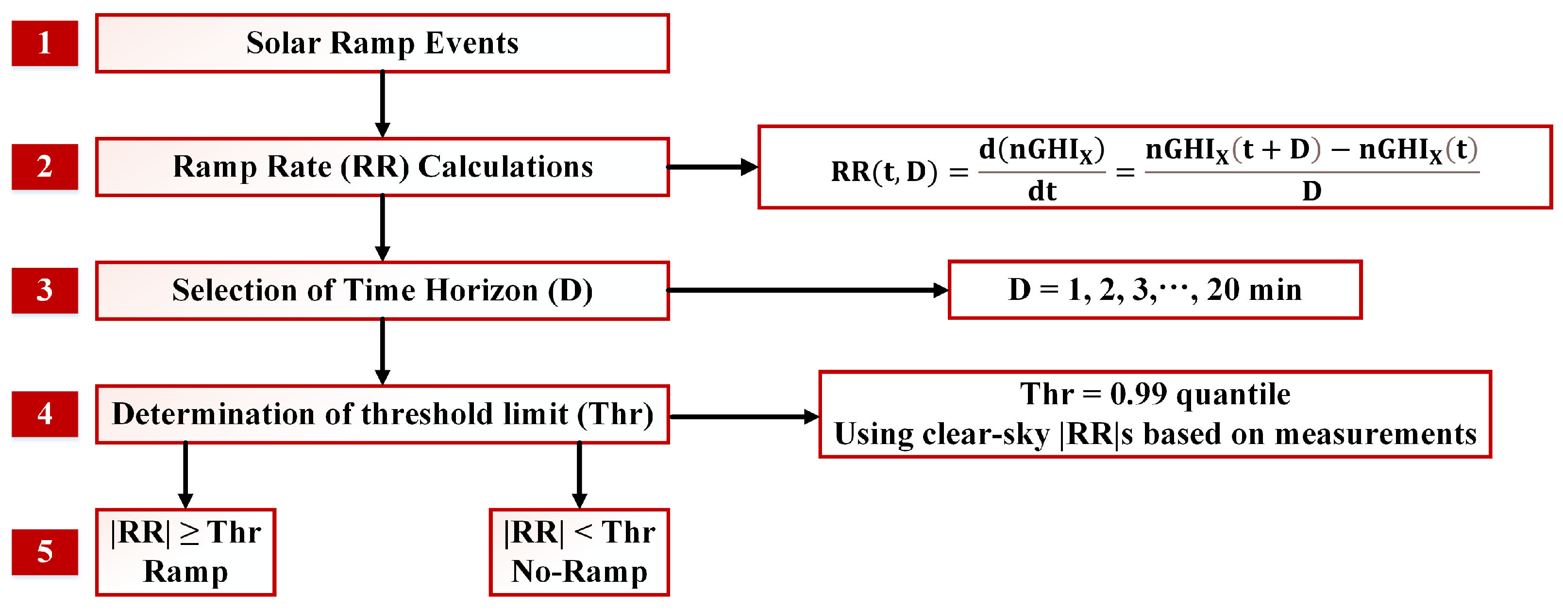
3.1. Characterization of Solar Irradiance Ramp Events

There is more than one definition of solar irradiance REs. The definition of an RE generally depends on the application. In this study, we aim to consider any case where transient clouds cause sudden changes of the incoming solar irradiance including both enhancement and reduction. The REs are detected through the calculation of the derivative of the normalized GHI (nGHI) from source X (reference measurement or ASI system forecast) ($nGH{I}_X$) (Equation (1)) at specific time horizons (ramp rate, RR) (Equation (2)),

$$nGH{I}_X=\frac{GH{I}_X}{{ϵ}_d},$$

(1)

$$RampRate=RR(t,D)=\frac{d\left(nGH{I}_X\right)}{dt}=\frac{nGH{I}_X(t+D)-nGH{I}_X\left(t\right)}{D},$$

(2)

where ${ϵ}_d$ is the maximum clear-sky GHI at the top of the atmosphere at each benchmark day, and $nGH{I}_X(t+D)$ is $nGH{I}_X$ at a future time step with time horizon D for the forecasted or the measured GHI. In addition, $nGH{I}_X\left(t\right)$ refers to the nGHI at the forecast issue time. The ${ϵ}_d$ is derived from the McClear model [30].

Figure 1 displays the flowchart of the implemented methodology for RE detection. The ramp events are determined as the exceedances of RR (calculated through steps 2 and 3) from a specific threshold limit (Thr) derived for each time horizon D through the 99th quantile of RR at clear skies, based on ground-based observations. In total, 23 days are considered to specify Thr. The former days are firstly selected by visual inspection of the all-sky images. Then, a clear-sky-detection methodology [31] is also performed to exclude potential timeframes with cloud presence.

Figure 2a represents the diurnal distribution of the clear-sky RRs for D = 10 min with similar results for other D values. During a clear-sky day, the magnitude of RR depends on the SZA indicating higher GHI variations for high SZAs. Figure 2b shows the Cumulative Distribution Function (CDF) of the clear-sky RR at D = 10 min. During a clear-sky day, the magnitude of RR depends on solar geometry indicating higher GHI variations for high SZAs encompassing a higher amplitude of RR. The 99th percentile of RR at clear skies represents the selected Thr (vertical line). At this point, the shape of the CDF changes as it approaches the knee point (Figure 2b), enabling the distinction of clear-sky RRs from possible cloudy RRs. In cases of many periods with cloud presence during an almost clear-sky day, a lower percentile for defining Thr should be presented. Therefore, the implemented methodology neglects the false ramp identification at low or high solar elevations. It is noted that this study focuses on predicting an RE regardless of its direction (up for positive RR or vice versa).

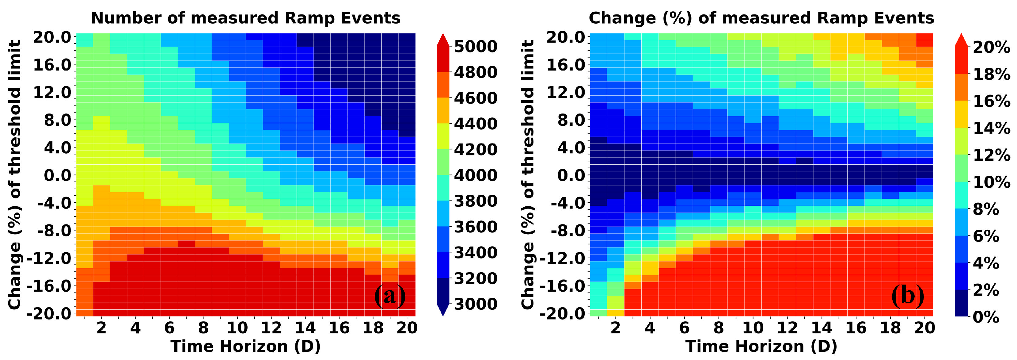
3.2. Sensitivity Analysis of Threshold Limits (Thr)

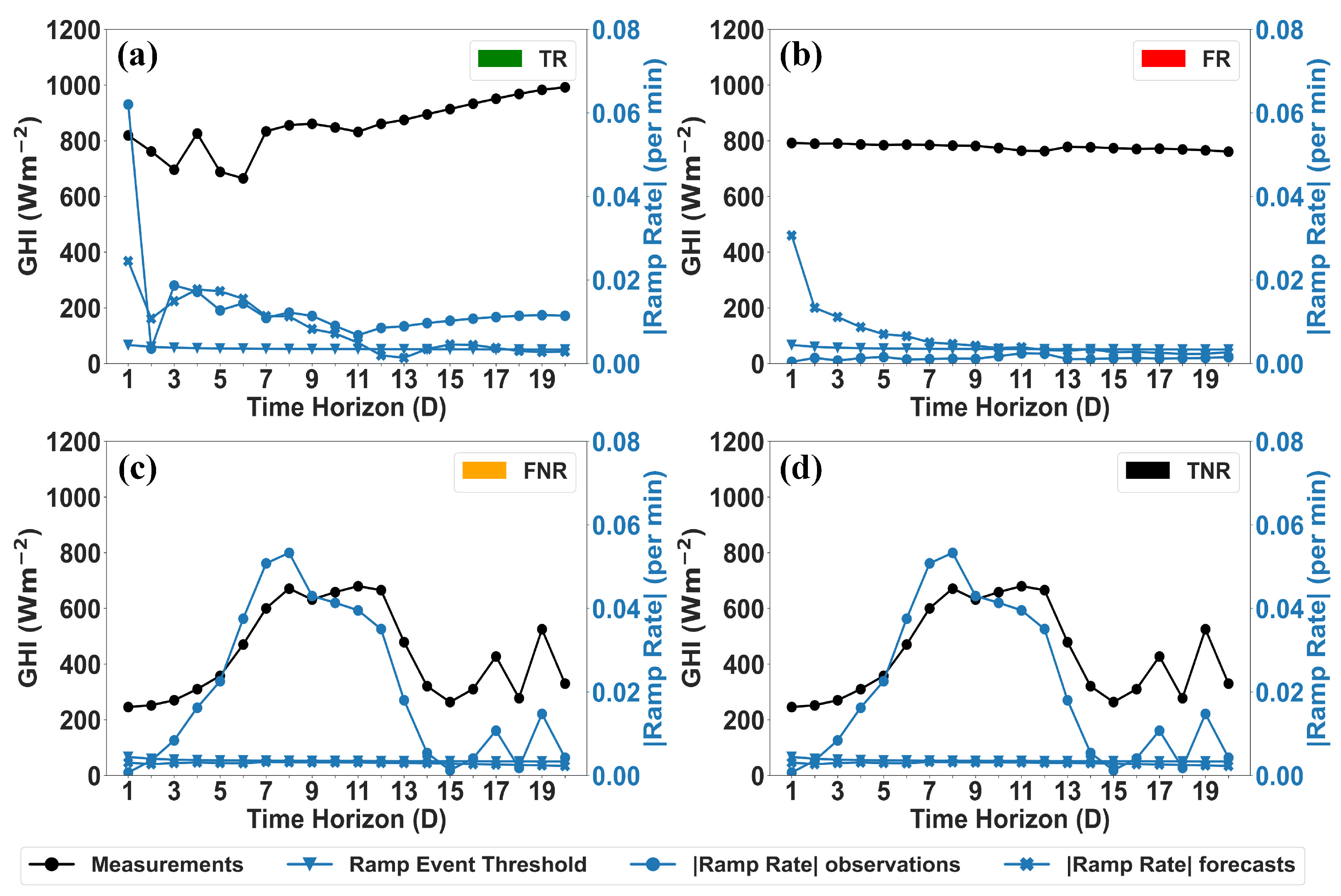
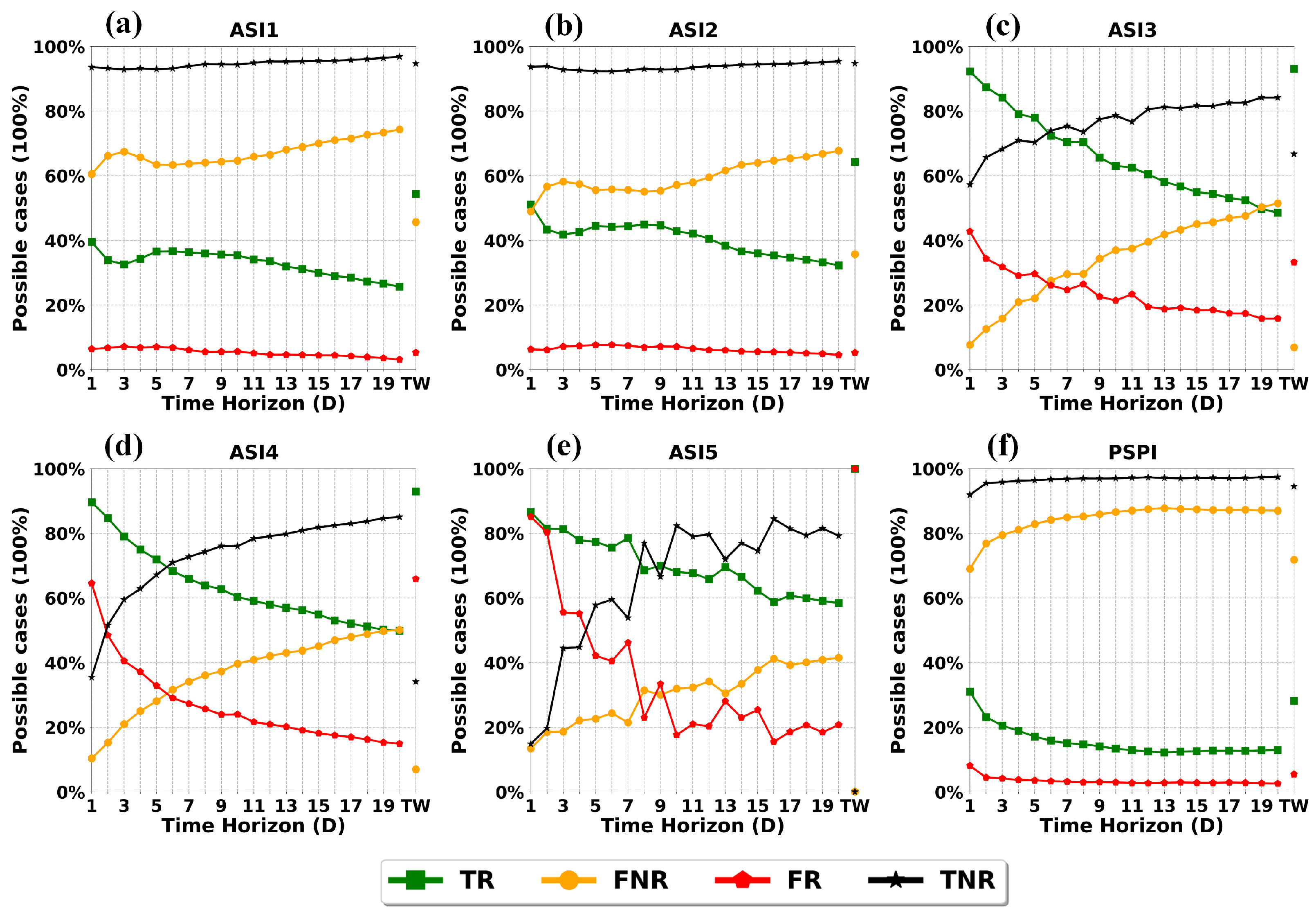
In this section, the robustness of the identification of REs is examined when changing the Thr by ±20% (Figure 3a). It is apparent that the number of REs increases for smaller Thr and vice versa. Nevertheless, the percentage change of measured REs (Figure 3b) for threshold changes within ±5% remains within ±8%, indicating adequately low variations around the initial number of REs (99th quantile). This methodology can be modified appropriately with different Thr levels depending on the application. For instance, if the purpose is to examine sudden solar irradiance fluctuations, a higher Thr value is desirable.

3.3. Possible Cases

Figure 4 illustrates an exemplary day including both clear and cloudy conditions. Under mostly clear skies (10:30–15:00 UTC), the applied methodology correctly detects the no-REs. Within other time frames of this day (up to 10:30 UTC and after 15:30 UTC), the presence of clouds leads to frequent sudden GHI changes.

The feasibility of ASIs to predict possible REs has been assessed both at specific D and over the whole 20 min time horizon denoted as “20 min time window analysis” or TW. RE of the observed GHI is the reference for comparison purposes.

Table 2. Confusion matrix of possible cases of forecasted ramp events.

		Observed Ramp Events
		Ramp	No-Ramp
Ramp Events	Ramp	True Ramp (TR)	False Ramp (FR)
Predicted	No-Ramp	False No-Ramp (FNR)	True No-Ramp (TNR)

shows the confusion matrix for the forecasted REs.

The diagonal elements of the confusion matrix represent the correctly detected ramp/no-ramp events (true ramp, TR, and true no-ramp, TNR). The off-diagonal values indicate erroneous predictions for the presence or absence of RE (false ramp, FR, and false no-ramp, FNR) using the ASI nowcasts. Regarding the 20 min window analysis, at least one RE is required (not restricted at the same D) by the ASIs and the measurements to assign a TR (Figure 5a). If no ramp is detected in the reference and the forecast for the 20 min window, a TNR is recorded (Figure 5d). FNR is denoted if the ASI nowcasts fail to predict any RE within the 20 min window although there is a ramp according to the pyranometer data (Figure 5c). FR is denoted if at least one RE is predicted by the ASIs although no ramp is found in the pyranometer reference data (Figure 5b). The implementation of the 20 min window to RE detection relies on the possible operational use of ASIs to inform the end-users about possible sudden GHI fluctuations. Restricting the analysis at specific D increases the possibility that FNR may cause a rapid reduction in grid power, leading to financial damages.

3.4. Goodness-of-Fit Statistics of Forecasted Ramp Events

Based on the confusion matrix results (Table 2), the qualitative performance of the forecasted REs is assessed using the following metrics:

$$TotalAccuracy=\frac{Truecases}{Totalcases}=\frac{TR+TNR}{TR+FR+FNR+TNR},$$

(3)

$$Precision=\frac{TR}{TR+FR},$$

(4)

$$Recall=\frac{TR}{TR+FNR},$$

(5)

$$F_{1}Score=\frac{2(Precision\times Recall)}{Precision+Recall},$$

(6)

4. Results

The results are presented in three sections. Section 4.1 describes the overall performance of the predicted REs relying on ASIs and PSPI nowcasts within different time horizons. Section 4.2 focuses on detecting intra-day REs under various cloud conditions. Section 4.3 outlines an insightful diurnal look of ASI-based RE detection for selected CC days.

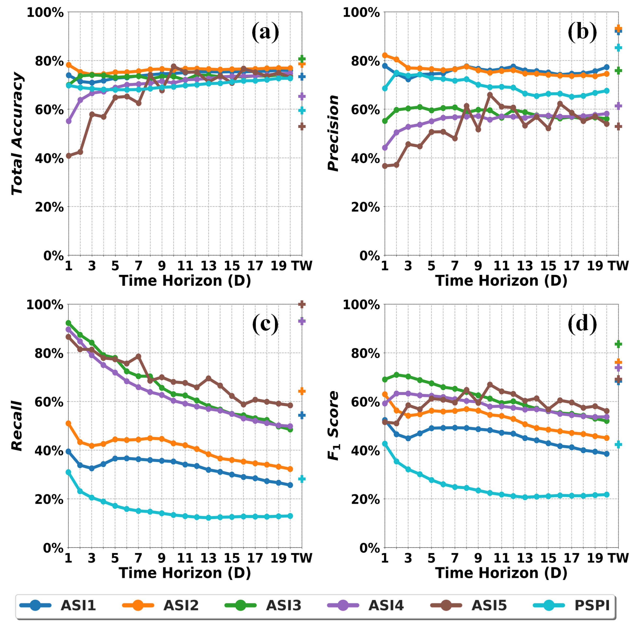
4.1. Overall Ramp Event-Detection Performance

Figure 6 displays the performance of algorithms in RE detection based on the 20 min window analysis. In general, forecast algorithms without cloud-cover information usually predict ramps based on time-interval lags [13,32]. In general, simple persistence model nowcasts are not able to capture any REs (Figure S1). Thus, the advanced persistence model, PSPI, used in this analysis predicts RE at times.

The total accuracy, namely the overall percentage of correct nowcasts (Equation (3)), is given above each confusion matrix (Figure 6). ASI3 and ASI2 show the highest total accuracy with 80.7% and 78.6%, respectively. Those two ASIs provide a contrasting result regarding the true RE “hits”. ASI3 outperforms ASI2 in TR event detection by 28.8%, while ASI2 is superior in TNR event detection by 27.9%. It should be mentioned that ASIs 1–2 systems are developed to provide spatial GHI forecasts and have been delimited only to a small area for the purposes of this benchmark, which penalizes the physical approach by means of geolocalization of clouds. RR-detection rates would increase significantly for these approaches if spatial information around the test side were considered [33]. Within the 20 min window analysis, ASI5 (Figure 6e) fails to distinguish the no-REs from the REs due to highly variable GHI forecasts during the clear-sky days.

Figure 7 presents the changes for all possible predicted cases (confusion matrix of Table 2) for the RE detection at increasing forecast time horizons and the entire time window, TW. Regardless of the possible cases (e.g., TR), the changes of the metrics with D are more intense for increasing time horizons and for algorithms based on deep-learning techniques (Figure 7c–e). Considering the TR events, the percentages of true detected cases decrease as the time horizon increases due to the reduction of GHI nowcast performance at distant time horizons (Figure 7). ASI1 and ASI2 can capture the TR cases in percentages ranging from 26.0% (Figure 7a, ASI1, D = 20 min) to 51.0% (Figure 7b, ASI2, D = 1 min).

Figure 8 shows accuracy, precision, recall and $F_1$ score for the forecasting systems as a function of D and for TW. As reported by the high precision scores (Figure 8b), ASI1 and ASI2 can avoid the FR “hits” (72.0–93.0%). On the other hand, their inability to detect some TR cases (FNR) leads to low recall scores Figure 8c, 26.0–39.0%). This behavior is due to merging of the image-based and persistence-based nowcasts used for ASI1 and ASI2. While the merging improves conventional error metrics such as RMSD, it reduces the variability of the forecasted irradiance. For ramp forecasts, an intermediate product of these ASI systems is advantageous, but this is not included in the evaluation of this work.

ASIs 3–5 can capture the TR event case reporting adequate good performances: scores higher than 50.0% are depicted in Figure 7c–e in most of the cases. The scores range from 49.0% (Figure 7c, ASI3, D = 20 min) to 92.0% (Figure 7c, ASI3, D = 1 min). Those algorithms avoid FNR “hits” presenting percentages from 8.0% (ASI3, D = 1 min) to 51.0% (ASI3, D = 20 min) and Recall scores between 48.0% and 92.0% (Figure 8c). However, their weakness in no-ramp (TNR) detection is revealed in the moderate precision scores (Figure 8b, 37.0–66.0%). When comparing the ASIs against the PSPI, ASI-based RE nowcasts are superior either for TNR (Figure 7a,b, ASIs 1-2) or TR (Figure 7, all ASIs) cases. Using the metrics mentioned above, the advances and drawbacks of each algorithm are thoroughly investigated. In addition to those metrics, the $F_1$ Score (Equation (6)) constitutes a valuable metric that compares the TR against false “hit” cases. For all algorithms except ASI5, the $F_1$ score decreases as the time horizon increases (Figure 8d). For short time horizons (D < 10 min), ASI3 outperforms the other algorithms, with $F_1$ score extending from 63.0% to 71.0%. At higher D, ASI5 shows the best performance, ranging between 56.0% and 66.0%. Among the algorithms, the PSPI provides the lowest $F_1$ score (Figure 8d, 22.0–43.0%), which is attributed to two reasons: (1) the relatively low TR percentages and (2) the quite high FNR percentages. The selection of the most suitable ASI system for solar irradiance RE nowcasting depends on the application. The different metrics can be used to assist in the selection of the most adequate system depending on the application.

4.2. Ramp Event-Detection Performance under Different Cloud Conditions

This section examines the differences in the RE forecast performance under various cloud conditions. (Figure 9 displays the minute-by-minute variability of the calculated metrics, as described in Section 3.4, separated into the six CCs (Table 1).

In terms of total accuracy, the revealed values and the best model’s performance differ at different cloud conditions. Under almost clear skies (Figure 9, CC: 1, 1st column 1st row), ASIs 1–2 and PSPI provide the highest scores (94.0–97.0%). In contrast, under overcast conditions (Figure 9, CC:4A, 1st column 6th row), ASIs 3–5 outperform the other models with accuracies ranging from 54.0% (ASI5) to 71.0% (ASI4). The RE-detection performance findings under the CCs coincide with the nowcast GHI validation analysis (see Figure 3 in Logothetis et al. [15]). For all models, the magnitude of total accuracy is decreased compared to clear-sky conditions, revealing the increased difficulty in RE detection for days with scattered clouds during half the day (CC: 3H) or throughout the whole day (2L-2H). Within the 20 min window analysis, ASI2, ASI3 and ASI5 outperform the other models in CCs 1 (92.0%) & 3H (85.0%), 2M (88.0%) & 2H (84.0%) and 2L (87.0%) & 4A (88.0%), respectively. On the other hand, PSPI provides the lowest scores (down to 26% in CC 4A) in most of the cases.

ASI1, ASI2 and PSPI record the highest precision scores, highlighting their ability to avoid the FR “hits” independently of the underlying cloud conditions (Figure 9, 2nd column). For CCs 2L-2H and overcast days, the increase of forecast time horizon indicates decreasing precision. In contrast, under clear-sky conditions, the increase of time horizon stands in favor of precision. In addition, the highest recall scores are reported for ASIs 3–5 (Figure 9, 3rd column), indicating their ability to avoid FNR “hits” at each CC. In contrast to precision, the recall metric decreases with increasing time horizons. The latter behavior of those algorithms is relevant to the increased FNR cases at distant time horizons. Finally, the highest $F_1$ scores (Figure 9, 3rd column 2nd-6th rows) are reported for ASIs 3–5, too.

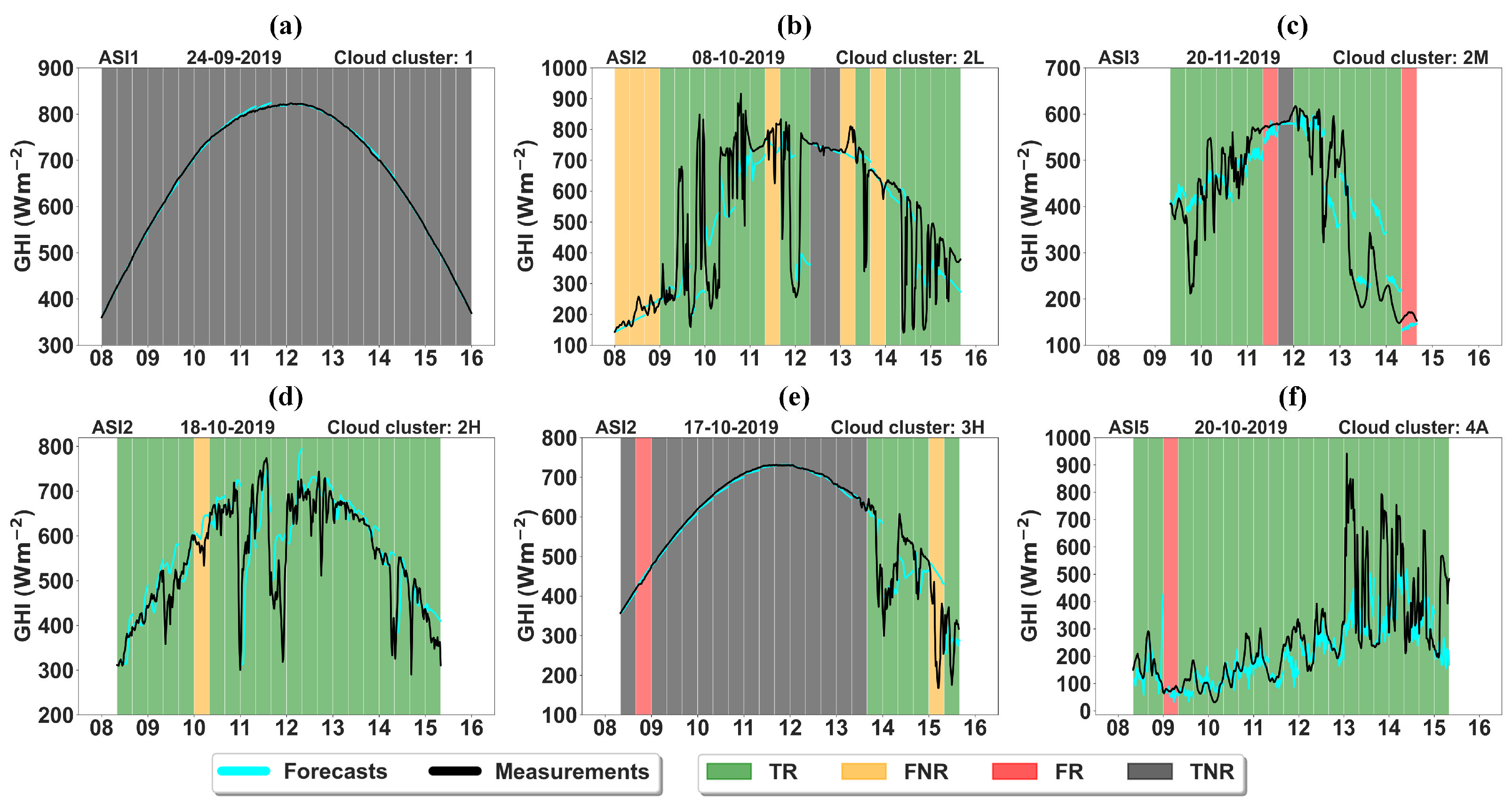
4.3. Intra-Day Variability of Ramp Event Forecasting for Selected Days and ASIs

A representative example for each CC day is also selected to investigate the diurnal performance of ASI-based RE nowcasts. The 20 min window analysis is applied to estimate the model’s performance in consecutive 20 min timeframes during each day. Figure 10 represents the results of the intra-day RE-detection variability for specific ASIs.

During the clear-sky day (CC: 1, Figure 10a), ASI1 can detect the TNR events correctly, capturing all the cases. Based on Figure 10b (CC: 2L), the scattered cloud conditions consisting of low height level clouds provide significant GHI changes; thus, most of the 20 min time windows include RE cases. During the CC 2L day, ASI2, whose algorithm is based on consecutive physical steps, can detect 15 out of 21 TRE cases and also correctly capture the two clear-sky timeframes (Figure 10b, 12:20–13:00 UTC).

Similar sudden GHI changes have also been observed during the CC 2M (Figure 10c) and 2H (Figure 10d) days. In CC 2M, the ASI3 tends to predict the RE cases for the whole day, showing weakness in avoiding the FR cases when clear-sky 20 min time periods exist (Figure 10c, 11:20–11:40 UTC etc.). Moreover, the ASI2 system predicts almost all TR cases (20 out of 21 TR cases) of the CC 2H day correctly (Figure 10d).

The CC 3H day (Figure 10e) is a very insightful case, including a half-day of almost clear-sky (up to 13:20 UTC) conditions along with a half-day of strong GHI fluctuations (after 13:20 UTC). On this day, ASI2 nowcasts reveal the best performance among ASIs regarding the true detected cases, documenting TNR and TR periods at 94.0% (15/16 cases) and 84.0% (5/6 cases). Similar results are observed for ASI1. During the CC 4A day, half of the day is under overcast cloud conditions (up to 13:00 UTC), where the detection of GHI fluctuations is a very challenging fact. The ASI5 relying on solely deep learning techniques report all the TR cases correctly.

5. Summary and Conclusions

For solar energy-dependent power systems, the ability to nowcast solar resource ramp events is important. A transient cloud can reduce the available solar energy abruptly, resulting in significant stability issues. The presented study was conducted within the framework of IEA PVPS Task 16 and utilizes the results from the first benchmarking exercise dealing with state-of-the-art solar nowcasting derived from ASIs. The benchmark took place at CIEMAT’s PSA in southern Spain, where four different ASI systems were installed and measured from August to November 2019. After validating the ASI-based nowcasts, their role concerning solar irradiance RE detection was investigated.

For the RE detection, the derivatives of the nGHI are calculated through specific timeframes (so-called ramp rates, RRs), spanning from 1 to 20 min in minute-by-minute increments. Next, an RE is defined by comparing the calculated RRs with predefined thresholds; their values were calculated under clear-sky conditions.

An interesting finding of this study is the connection between the detected ramp events and the applied ASI-based forecast algorithms. ASIs are able to predict about 55 to nearly 100% of the ramp events. ASIs 1–2 and 3–5 predict 55–65% and 90% to nearly 100% of all ramp events, respectively. It should be noted that ASI 1–2 systems were designed to produce spatial GHI forecasts and were merely confined to a narrow area for the sake of this benchmark, which penalizes the physical approach, especially by means of geolocalization of clouds. Including a wider area of GHI forecasts results in a higher true ramp event-detection performance. ASIs 3–5 show the tendency to falsely predict ramp events, which happens less often for ASI1 and ASI2. For both categories, the number of true ramp event cases decreases with increasing forecasting horizon. The total ramp forecast accuracy reaches up to about 80% for both categories of forecast systems (ASI2, ASI3).

The RE-detection analysis is also performed under different cloud conditions. The results indicate a strong relationship between the accuracy of the ramp forecast and the underlying cloud conditions. Within the 20 min window analysis, for the days with scattered cloudiness or overcast conditions, the deep-learning algorithms (ASIs 3–5) outperform the other algorithms, presenting scores up to 88.0%. In contrast, in days with scattered cloudiness during half the day and cloudlessness during the other half, the systems that apply consecutive physical steps outperform the other algorithms.

It is also of interest to compare the findings related to the ramp forecasting accuracy to an analysis focusing on other conventional forecasting metrics, namely bias, RMSD and MAD (mean absolute deviation) (see Logothetis et al. [15]). In this previous analysis, ASI 2 was the system that had the best performance in MAD and RSMD for most cloud clusters. All ASI systems performed well compared to persistence forecasts and had a low bias. The physically based systems, ASI1 and 2, outperformed the persistence models at all cloud clusters and lead times. For lead times longer than 5 min, the deep-learning systems (ASIs 3–5) are also efficient enough to outperform the persistence model under cloudy skies.

The selection of the most suitable ASI system for solar irradiance RE nowcasting depends on the application. Some systems provide better ramp forecasts in terms of recall, others in terms of precision or total accuracy of the ramp forecasts, RMSD or MAD. No single system or system category (e.g., deep learning, or physical) performs best in all metrics and hence all applications. The different metrics can be used to assist in the selection of the most adequate system depending on the application. Moreover, these findings indicate that the combination of several evaluation approaches based on the same images and radiation data could be beneficial. It might be of interest to provide separate ramp forecasts, that consider more information than the user can derive from the final irradiance forecast alone.

The inability of the reference models, like persistence, to capture sudden solar fluctuations demands alternative approaches. This study presents a different means of predicting solar radiation REs, enabling an in-depth investigation of ASI-based nowcasts. The findings of this study highlight the feasibility of ASI solar irradiance nowcasts in terms of predicting REs. Therefore, ASI systems could be introduced as an integrated tool for solar technologies that provide emergency calls during periods of strong power fluctuations, reducing financial costs and improving efficiency.

References

1. Bianco, L.; Djalalova, V.I.; Wilczak, M.J.; Cline, J.; Calvert, S.; Konopleva-Akish, E.; Finley, C.; Freedman, J. A Wind Energy Ramp Tool and Metric for Measuring the Skill of Numerical Weather Prediction Models. Weather. Forecast. 2016, 31, 1137–1156. [Google Scholar] [CrossRef]
2. Kamath, C. Understanding wind ramp events through analysis of historical data. In Proceedings of the Transmission and Distribution Conference and Exposition, New Orleans, LA, USA, 19–22 April 2010; IEEE: Piscataway, NJ, USA, 2010. [Google Scholar] [CrossRef]
3. Ferreira, C.; Gamma, J.; Matias, L.; Botteud, A.; Wang, J. A Survey on Wind Power Ramp Forecasting; Argonne National Laboratory Rep. ANL/DIS-10-13; Argonne National Lab: Argonne, IL, USA, 2011; p. 28. Available online: http://ceeesa.es.anl.gov/pubs/69166.pdf (accessed on 24 August 2022).
4. Cui, M.; Zhang, L.; Feng, C.; Florita, A.R.; Sun, Y.; Hodge, B.M. Characterizing and analyzing ramping events in wind power, solar power, load, and net load. Renew. Energy 2017, 111, 227–244. [Google Scholar] [CrossRef]
5. Abuella, M.; Chowdhury, B. Forecasting of solar power ramp events: A post-processing approach. Renew. Energy 2019, 133, 1380–1392. [Google Scholar] [CrossRef]
6. Kong, W.; Jia, Y.; Dong, Z.Y.; Meng, K.; Chai, S. Hybrid approaches based on deepwhole-sky-image learning to photovoltaic generation forecasting. Appl. Energy 2020, 280, 115875. [Google Scholar] [CrossRef]
7. Florita, A.; Hodge, B.; Orwig, K. Identifying wind and solar ramping events. In Proceedings of the 2013 IEEE Green Technologies Conference (GreenTech), Denver, CO, USA, 4–5 April 2013; pp. 147–152. [Google Scholar] [CrossRef]
8. Bristol, E. Swinging door trending: Adaptive trend recording? In Proceedings of the ISA National Conference Proceedings, Sydney, Australia; 1990; Volume 45, pp. 749–753. [Google Scholar]
9. Vallance, L.; Charbonnier, B.; Paul, N.; Dubost, S.; Blanc, P. Towards a standardized procedure to assess solar forecast accuracy: A new ramp and time alignment metric. Sol. Energy 2017, 150, 408–422. [Google Scholar] [CrossRef]
10. Cui, M.; Zhang, J.; Florita, A.R.; Hodge, B.M.; Ke, D.; Sun, R. An optimized swinging door algorithm for identifying wind ramping events. IEEE Trans. Sustain. Energy 2016, 7, 150–162. [Google Scholar] [CrossRef]
11. Abuella, M.; Chowdhury, B. Forecasting Solar Power Ramp Events Using Machine Learning Classification Techniques. In Proceedings of the 2018 IEEE 9th International Symposium on Power Electronics for Distributed Generation Systems (PEDG), Charlotte, NC, USA, 25–28 June 2018; pp. 1–6. [Google Scholar] [CrossRef]
12. Reno, M.J.; Stein, J.S. Using Cloud Classification to Model Solar Variability; Sandia National Lab: Albuquerque, NM, USA, 2013. [CrossRef]
13. Chu, Y.; Pedro, H.T.C.; Li, M.; Coimbra, C.F.M. Real-time forecasting of solar irradiance ramps with smart image processing. Sol. Energy 2015, 114, 91–104. [Google Scholar] [CrossRef]
14. Caldas, M.; Alonso-Suárez, R. Very short-term solar irradiance forecast using all-sky imaging and real-time irradiance measurements. Renew. Energy 2019, 143, 1643–1658. [Google Scholar] [CrossRef]
15. Logothetis, S.A.; Salamalikis, V.; Wilbert, S.; Remund, J.; Zarzalejo, F.L.; Xie, Y.; Nouri, B.; Ntavelis, E.; Nou, J.; Hendrikx, N.; et al. Benchmarking of solar irradiance nowcast performance derived from all-sky imagers. Renew. Energy 2022. under review. [Google Scholar]
16. Wilbert, S.; Nouri, B.; Prahl, C.; Garcia, G.; Ramirez, L.; Zarzalejo, F.L.; Valenzuela, X.R.; Ferrera, F.; Kozonek, N.; Liria, J. Application of Whole Sky Imagers for Data Selection for Radiometer Calibration. In Proceedings of the EUPVSEC, Munich, Germany, 20–24 June 2016. [Google Scholar]
17. Fabel, Y.; Nouri, B.; Wilbert, S.; Blum, N.; Triebel, R.; Hasenbalg, M.; Kuhn, P.; Zarzalejo, L.F.; Pitz-Paal, R. Applying self-supervised learning for semantic cloud segmentation of all-sky images. Atmos. Meas. Tech. 2022, 15, 797–809. [Google Scholar] [CrossRef]
18. Nouri, B.; Noureldin, K.; Schlichting, T.; Wilbert, S.; Hirsch, T.; Schroedter-Homscheidt, M.; Kuhn, P.; Kazantzidis, A.; Zarzalejo, L.F.; Blanc, P.; et al. A way to increase parabolic trough plant yield by roughly 2% using all sky imager derived DNI maps. AIP Conf. Proc. 2020, 2303, 110005. [Google Scholar] [CrossRef]
19. Nouri, B.; Kuhn, P.; Wilbert, S.; Hanrieder, N.; Prahl, C.; Zarzalejo, L.F.; Kazantzidis, A.; Blanc, P.; Pitz-Paal, R. Cloud height and tracking accuracy of three all sky imager systems for individual clouds. Sol. Energy 2019, 177, 213–228. [Google Scholar] [CrossRef]
20. Nouri, B. Solar Irradiance Nowcasting System to Optimize the Yield in Parabolic trough Power Plants. [Solarstrahlungs-Kürzestfrist-Vorhersagesystem für die Ertragsoptimierung eines Parabolrinnenkraftwerks]. Ph.D. Thesis, RWTH Aachen, Aachen, Germany, 2020. [Google Scholar]
21. Nouri, B.; Wilbert, S.; Segura, L.; Kuhn, P.; Hanrieder, N.; Kazantzidis, A.; Schmidt, T.; Zarzalejo, L.; Blanc, P.; Pitz-Paal, R. Determination of cloud transmittance for all sky imager based solar nowcasting. Sol. Energy 2019, 181, 251–263. [Google Scholar] [CrossRef]
22. Nouri, B.; Blum, N.; Wilbert, S.; Zarzalejo, L.F. A hybrid solar irradiance nowcasting approach: Combining all sky imager systems and persistence irradiance models for increased accuracy. Sol. RRL 2021, 6, 2100442. [Google Scholar] [CrossRef]
23. Nou, J.; Chauvin, R.; Thil, S.; Grieu, S. A new approach to the real-time assessment of the clear-sky DNI. Appl. Math. Model. 2016, 40, 7245–7264. [Google Scholar] [CrossRef]
24. Chauvin, R.; Nou, J.; Thil, S.; Grieu, S. System for Measuring Components of Solar Radiation. Patent WO2019053232, 21 March 2019. [Google Scholar]
25. Hendrikx, N.H.; Visser, L.R.; P.ó, M.; Salah, A.A.; van Sark, W.G.J.H.M. All sky imaging based short-term solar irradiance forecasting with Long Short-Term Memory networks. 2022; in preparation. [Google Scholar]
26. Chauvin, R.; Nou, J.; Thil, S.; Traoré, A.; Grieu, S. Cloud Detection Methodology Based on a Sky-imaging System. Energy Procedia 2015, 69, 1970–1980. [Google Scholar] [CrossRef]
27. Canny, J. A computational approach to edge detection. IEEE Trans. Pattern Anal. Mach. Intell. 1986, 6, 679–698. [Google Scholar] [CrossRef]
28. Shapiro, L.; Stockman, G. Computer Vision; Prentice-Hall, Inc.: Upper Saddle River, NJ, USA, 2001. [Google Scholar]
29. Kumler, A.; Xie, Y.; Zhang, Y. A Physics-based Smart Persistence model for Intra-hour forecasting of solar radiation (PSPI) using GHI measurements and a cloud retrieval technique. Sol. Energy 2019, 177, 494–500. [Google Scholar] [CrossRef]
30. Lefèvre, M.; Oumbe, A.; Blanc, P.; Espinar, B.; Gschwind, B.; Qu, Z.; Wald, L.; Schroedter-Homscheidt, M.; Hoyer-Klick, C.; Arola, A.; et al. McClear: A new model estimating downwelling solar radiation at ground level in clear-sky conditions. Atmos. Meas. Tech. 2013, 6, 2403–2418. [Google Scholar] [CrossRef]
31. Reno, M.J.; Hansen, C.W. Identification of periods of clear sky irradiance intime series of GHI measurements. Renew. Energy 2016, 90, 520–531. [Google Scholar] [CrossRef]
32. Chu, Y.; Li, M.; Coimbra, C.F.M.; Feng, D.; Wang, H. Intra-hour irradiance forecasting techniques for solar power integration: A review. iScience 2021, 24, 103136. [Google Scholar] [CrossRef] [PubMed]
33. Fabel, Y.; Nouri, B.; Wilbert, S.; Antonio Caballo, J.; Blum, N.; Zarzalejo, L.F.; Ugedo Egido, E.; Pitz-Paal, R. Solar Nowcasting Systems Using AI Techniques. In Proceedings of the 25th Cologne Solar Colloquium, Jülich, Germany, 22 June 2022. [Google Scholar]
Figure 1. Flowchart of the applied methodology.
Energies 15 06191 g001
Figure 2. (a) Scatter plot and (b) CDF function of ramp rates (RRs) for clear-sky conditions at time horizon D=10 min. The solid black lines indicate the threshold limit (99th quantile) that classifies the no-ramp (red area) and ramp (green area) events. The blueish color bar refers to the solar zenith angle.
Energies 15 06191 g002
Figure 3. (a) Total number of measured ramp events and (b) the change of this number caused by varying the threshold limit (Thr) at each time horizon (D). The vertical axis shows the change of the threshold limit, whereas the horizontal axis presents D. The color bar displays the number of ramp events (a) and the change of the number of ramp events (b).
Energies 15 06191 g003
Figure 4. The graph in the upper panel depicts the intra-day GHI variability and the absolute observed ramp rate values at time horizon D = 1 min derived from the reference pyranometer. The red horizontal line corresponds to the threshold limit for D = 1 min. The lower four plots show the detected ramp events based on ground-based measurements in four time intervals: (a) 08:00–10:00, (b) 10:00–12:00, (c) 12:00–14:00 and (d) 14:00–16:00.
Energies 15 06191 g004
Figure 5. Example of ramp rate values within a 20 min window of ASI nowcasts for (a) True Ramp event (TR), (b) False Ramp Event (FR), (c) False No-Ramp Event (FNR) and (d) True No-Ramp Event (TNR). The black line refers to the measured GHI. The blue lines correspond to the ramp event threshold (∇ symbol) and the calculated absolute ramp rates from ASI forecasts (× symbol) and measurements (• symbol), respectively.
Energies 15 06191 g005
Figure 6. Confusion matrix including all possible cases of Table 2 for (a) ASI1, (b) ASI2, (c) ASI3, (d) ASI4, (e) ASI5 and (f) PSPI. The percentages of each quadrant are calculated based on the true measured cases (either for ramp or no-ramp events) and refer to the ramp event detection within the 20 min window analysis (see Section 3.3).
Energies 15 06191 g006
Figure 7. Variability of all predicted possible cases of Table 2 as well as at the 20-minute time window (TW) for (a) ASI1, (b) ASI2, (c) ASI3, (d) ASI4, (e) ASI5 and (f) PSPI. The time horizon begins from 1 min and reaches 20 min in minute-by-minute increments. The percentages of each Table 2 quadrant are calculated based on the true measured cases (either for the ramp or no-ramp events). TR = True Ramp, FNR = False No-Ramp, FR = False Ramp and TNR = True No-Ramp.
Energies 15 06191 g007
Figure 8. (a) Total Accuracy, (b) Precision, (c) Recall and (d) F 1 Score, for each ASI system and PSPI. Each metric is calculated at each time horizon D (solid lines) as well as at the 20 min time window analysis (TW + symbol). The definition of each metric is presented in Section 3.4. All metrics are presented as percentages.
Energies 15 06191 g008
Figure 9. Total Accuracy (1st column), Precision (2nd column), Recall (3rd column) and F1 Score (4th column) for cloud clusters: 1 (1st row), 2L (2nd row), 2M (3rd row), 2H (4th row), 3H (5th row) and 4A (6th row). Each metric is calculated at each time horizon D (up to 20 min, solid lines) and the 20 min time window (TW, star symbol). The definition of each cloud cluster is presented in Section 2.
Energies 15 06191 g009
Figure 10. Intra-day variability of the four possible ramp event-detection cases included in Table 2 for the 20 min window analysis, TW, at selected days and ASIs for cloud cluster: (a) 1, (b) 2L, (c) 2M, (d) 2H, (e) 3H and (f) 4A. For the sake of clarity and to ensure continuity, the presented 20 min windows include the ramp event nowcasts having as a starting forecast time point the exact time (e.g., 08:00, 08:20 UTC, etc.) and containing up to 20 min (e.g., 08:01–08:20, 08:21–08:40 UTC, etc.) in minute-by-minute increments. The background colors in each graph correspond to the four possible cases in Table 2. The solid black and cyan lines correspond to measured GHI and model-based GHI nowcasts within each 20 min window.
Energies 15 06191 g010