Short-Term Wind Power Prediction Based on LightGBM and Meteorological Reanalysis

Abstract

With the expansion of wind power grid integration, the challenges of sharp fluctuations and high uncertainty in preparing the power grid day-ahead plan and short-term dispatching are magnified. These challenges can be overcome through accurate short-term wind power process prediction based on mining historical operation data and taking full advantage of meteorological forecast information. In this paper, adopting the ERA5 reanalysis dataset as input, a short-term wind power prediction framework is proposed, combining light gradient boosting machine (LightGBM), mutual information coefficient (MIC) and nonparametric regression. Primarily, the reanalysis data of ERA5 provide more meteorological information for the framework, which can help improve the model input features. Furthermore, MIC can identify effective feature subsets from massive feature sets that significantly affect the output, enabling concise understanding of the output. Moreover, LightGBM is a prediction method with a stronger ability of goodness-of-fit, which can fully mine the effective information of wind power historical operation data to improve the prediction accuracy. Eventually, nonparametric regression expands the process prediction to interval prediction, which significantly improves the utility of the prediction results. To quantitatively analyze the prediction results, five evaluation criteria are used, namely, the Pearson correlation coefficient (CORR), the root mean square error (RMSE), the mean absolute error (MAE), the index of agreement (IA) and Kling–Gupta efficiency (KGE). Compared with support vector regression (SVR), random forest (RF) and extreme gradient boosting (XGBoost) models, the present framework can make full use of meteorological information and effectively improve the prediction accuracy, and the generated output prediction interval can also be used to promote the safe operation of power systems.

1. Introduction

With the popularization of the concept of sustainable development, nonpolluting wind energy has received an increasing amount of attention in China. The installed capacity of wind power in China reached 3.3 × 10⁸ kW at the end of 2021, with a growth rate of 16.7% compared with 2020, accounting for 50.91% of the global newly installed capacity, ranking first in the world [1]. At the same time, the problem of wind power curtailment is becoming increasingly serious. China’s wind power curtailment in 2019 and 2020 reached 16.86 billion kWh and 16.60 billion kWh, respectively, and increased to 20.61 billion kWh in 2021, almost one-fifth of the wind power generation in the U.K., causing a great waste of social resources [2]. Accurate wind power generation process forecasting is an important measure to reduce wind curtailment and achieve economic operation. However, due to the large scale of wind power integration and the uncertainty of meteorological forecasting, it is difficult to ensure the accuracy of wind power prediction [3,4], which is not conducive to the preparation of power grid day-ahead plan and short-term dispatching [5].

The prediction of wind power processes for sustainable development has become a key academic field in recent years. Feng et al. proposed a multi-model wind forecasting methodology and developed a deep feature selection framework to determine the input of historical data [6]. Yuan et al. forecasted the nonlinear component of wind power series by making use of wind speed, wind direction and residual error series of the autoregressive fractionally integrated moving average model [7]. The methods make predictions relying on historical wind power and wind speed data, and it is difficult to make accurate predictions without considering the uncertainty of wind power caused by changes due to other meteorological factors [8]. Wind power prediction that takes meteorological factors into account has been shown to minimize fluctuations in wind power and increase the prediction accuracy [9]. The mainstream meteorological factors related to wind power in academia include atmospheric pressure, temperature and humidity [10,11]. Jahangir et al. established a multimodal short-term wind speed prediction framework considering three kinds of meteorological data, and utilized a sinusoidal rough neural network (SR-NN) for wind speed prediction [12]. Zameer et al. [13] applied the intelligent ensemble regressor of artificial neural networks and genetic programming to reduce the impact of frequent fluctuations of temperature and other meteorological data on regression analysis. Guo et al. [14] proposed a new wind speed prediction method based on the a priori algorithm. This method can effectively discover the association rules among wind speed, temperature and humidity; these correlations can then be employed to predict and correct wind speed data. However, the interfering factors of wind power output are complex. The above authors did not sufficiently consider important data for meteorological factors, including the elevation difference between wind speed and temperature observations, and the influence of additional meteorological factors. In addition, the meteorological products they selected are relatively outdated, which will affect the accuracy of the data obtained. All these considerations leave room for improvement in the prediction accuracy.

To predict wind power, it is necessary to uncover relevant information in historical data. This requires the thoughtful development of new strategies. Data-driven modeling has become an important tool in academia because of its adaptability to short-term prediction and its efficient simulation of nonlinear output processes [15]. It is applied broadly in the mining of relevant information, wind power and solar energy prediction, and other fields [16,17], and is the topic of research in this article. Machine learning methods have recently had an impact on output prediction, such as neural networks [18], support vector regression [19] and random forests [20]. Wind power prediction is a multi-input and multistage optimization decision-making process. The data structure is complex, and the scale of the calculation problem is large [21], which makes the traditional algorithms unable to meet the prediction requirements. Light gradient boosting machine (LightGBM) is a new distributed gradient lifting framework based on a decision tree algorithm. It can fully mine the hidden information of random sequences and has the advantages of fast calculation speed and strong robustness. For these reasons, the usefulness of LightGBM in the prediction of power is promising. Park et al. [22] proved that LightGBM has better prediction performance than other methods built upon decision trees. Ju et al. stated that LightGBM has been widely applied to data scientific processing [23]. Musbah et al. employed LightGBM to predict the combination mode of energy, and achieved suitable results in power supply stability [24]. Although studies have proven the reliability of LightGBM in many aspects of wind power prediction, how to incorporate more input factors into the model remains an important research question.

The prediction of wind power output also needs to determine all pertinent meteorological factors and obtain these data accurately. Studies of the impact of meteorological factors on wind power prediction have primarily focused on wind speed, wind direction, pressure and temperature. Since the relationship between wind power generation and meteorological factors is complex, it is still necessary for researchers to mine and analyze the influence of additional meteorological factors on wind power output. Compared with Pearson, Spearman, Kendall and other measures of correlation between two variables, the maximal information coefficient (MIC) has the advantages of stronger robustness and better fairness. It is more suitable for the correlation analysis of nonlinear time series of meteorological data and has attracted much attention in academic research [25]. Therefore, the application of MIC can identify effective feature subsets from massive feature sets. Meteorological variables are usually obtained through a numerical weather prediction (NWP) system, and the data received from NWP systems may contain errors. In addition, owing to the need for continuous improvement of the prediction system, scholars have struggled to obtain long sequences of consistent data [26]. To mitigate these problems, the reanalysis data provided by the latest meteorological product, ECMWF Reanalysis v5 (ERA5), are used in this study. The reanalysis data contain fewer errors than the observed data and forecast data, and can satisfy the prerequisites for long sequences of consistent data [27].

In this paper, MIC is utilized to select input factors with high correlation with wind power output from ERA5 meteorological reanalysis data, which ensures that ample information is supplied to the prediction model while avoiding the inefficient use of computing resources caused by feature redundancy. LightGBM, which has a strong nonlinear fitting ability, acts as the prediction method to improve the forecasting accuracy. The output prediction interval is generated through a nonparametric regression method, and the prediction results are tested at different confidence interval levels. The results of the study show that the method proposed in this paper can improve the prediction accuracy and provide relevant information for the safe operation of power grids.

2. Data Acquisition

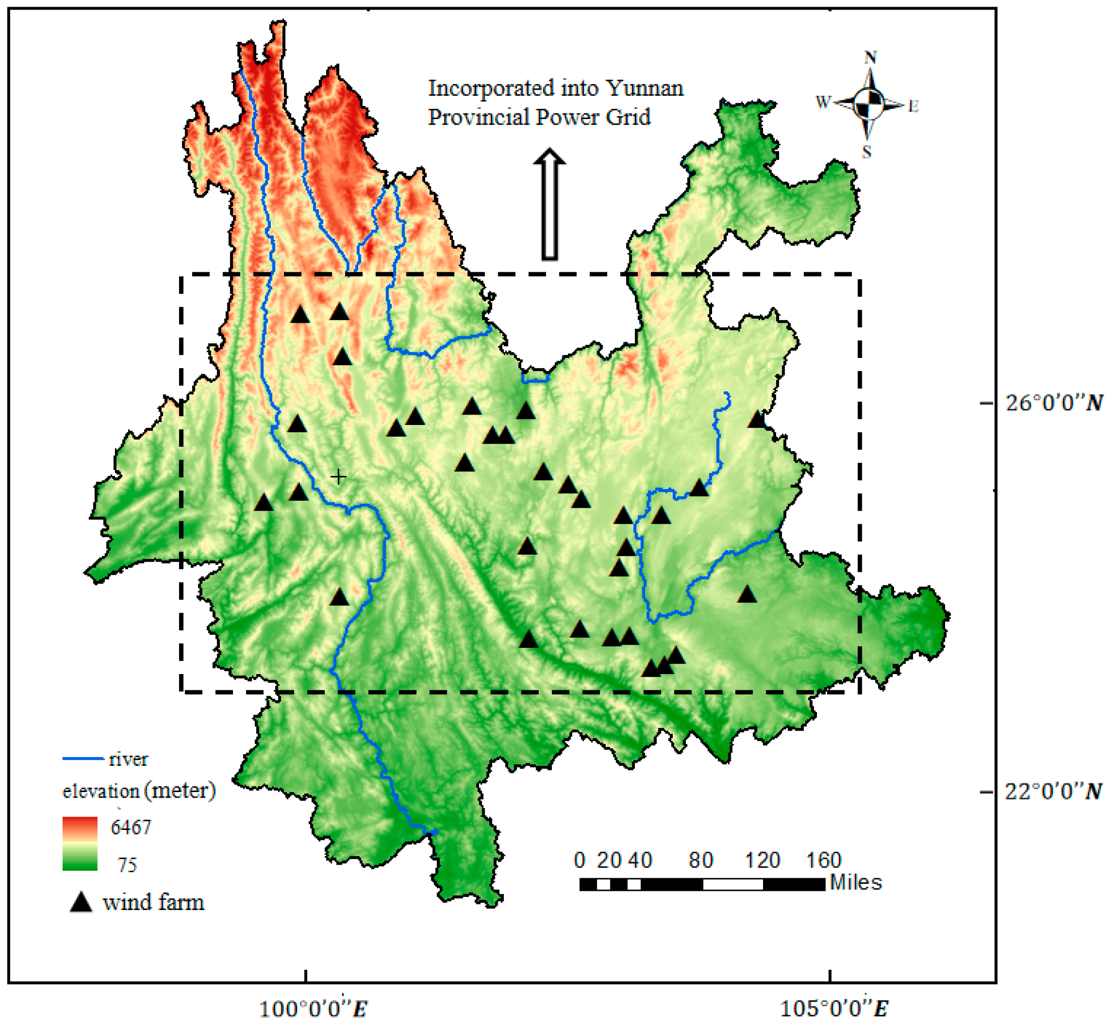
2.1. Data Introduction

Yunnan Province of China was selected as the research site. Yunnan is located in southeastern Eurasia, with the world’s largest plateau, Qinghai Tibet Plateau, in the northwest and the ocean to the south. It is located in a typical monsoon climate zone, and the terrain of the province tends to be high in the northwest and low in the southeast. In winter, because the mainland is cold and the ocean is warm, the wind blows from the mainland to the ocean. Due to the obstruction of the Iranian Plateau and the Qinghai Tibet Plateau, the airflow in Yunnan bypasses into a westerly wind. Therefore, dry westerly winds prevail in most areas of Yunnan in the colder half of the year. In summer, the continent is warm and the ocean is cold. The wind blows from the ocean to the continent, and the southwest flow of air from the Indian Ocean blows to Yunnan through the Bay of Bengal. Therefore, Yunnan enjoys a humid ocean southwest monsoon in summer. Figure 1 shows the large-scale wind farms with more than 50 MW in Yunnan Province, which are generally distributed horizontally.

As a major energy-producing province in China, Yunnan Province has made great progress in the wind–solar–water multi-energy complementary system, with a high level of reliance on clean energy. At the end of 2020, the installed power generation capacity of the province was approximately 1.034 × 10⁸ kW, an increase of 8.4 × 10⁶ kW from the previous year. The wind power capacity was 8.8 × 10⁶ kW, accounting for 8.5% of the total capacity [28]. The total wind power output of Yunnan Province in 2020 was collected in this study. The output data interval was 15 min, with a total of 35,040 data points. The data from 8 o’clock on 1 January 2020 to 8 o’clock on 26 July 2020 were used as training data. The data from 8 o’clock on 26 July 2020 to 8 o’clock on 15 October 2020 were used as validation data. The data from 8 o’clock on 15 October 2020 to 8 o’clock on 31 December 2020 were used as test data. The percentages of training, validation and testing data were approximately 60%, 20% and 20%, respectively.

2.2. Meteorological Data

Meteorological factors were selected in this study with two goals. The first was to further refine the known relevant meteorological factors; the second was to identify new meteorological factors that may be relevant. ERA5 is the latest comprehensive meteorological data product. Compared with ERA-interim and other products, it can provide more kinds of meteorological data and with greater accuracy. In this study, ERA5 meteorological reanalysis data acquisition is as follows: “ERA5 hourly data on single levels from 1959 to present. Available online: https://cds.climate.copernicus.eu/cdsapp#!/dataset/reanalysis-era5-single-levels?tab=form (accessed on 7 May 2021)”. Data were provided every 1 h on a 0.25° × 0.25° spatial grid. Reanalysis data are “comprehensive” data that integrate ground station observation, satellite remote sensing and numerical model simulation. Reanalysis uses the data that already occurred to adjust the original model parameters and then re-forecast. In short, reanalysis data are the data obtained after the quality control of the observed data and then assimilation into the global model. According to expert knowledge and the existing literature, 23 meteorological factors were considered as predictors of wind power output (

Table 1. The selection results of meteorological factors.

No.	Variable	Description	Units
1	u100	West wind at 100 m elevation	m · s−1
2	v100	South wind at 100 m elevation	m · s−1
3	u10n	West wind of neutral wind at 10 m elevation	m · s−1
4	u10	West wind at 10 m elevation	m · s−1
5	v10n	South wind of neutral wind at 10 m elevation	m · s−1
6	v10	South wind at 10 m elevation	m · s−1
7	fg10	10 m wind gust since previous post-processing (since the parameter was last archived in a particular forecast)	m · s−1
8	d2m	2 m dewpoint temperature	K
9	t2m	2 m temperature	K
10	i10fg	Instantaneous 10 m wind gust	m · s−1
11	cdir	Clear-sky direct solar radiation at surface	J · m−2
12	e	Evaporation	mm
13	mx2t	Maximum 2 m temperature since previous post-processing	K
14	megwss	Mean eastward gravity wave surface stress	N · m−2
15	mgwd	Mean gravity wave dissipation	W · m−2
16	mngwss	Mean northward gravity wave surface stress	N · m−2
17	mn2t	Minimum 2 m temperature since previous post-processing	K
18	skt	Skin temperature	K
19	es	Snow evaporation	mm
20	stl1	Soil temperature level 1	K
21	slhf	Surface latent heat flux	J · m−2
22	sp	Surface pressure	Pa
23	p59	Mean eastward turbulent surface stress	N · m−2

).

3. Methodology

3.1. Noise Reduction of Wind Power Generation

In practice, there is always a certain amount of error in measured output data, referred to as noise, due to natural and human factors. Noise seriously affects the convergence rate of data and reduces the accuracy of quantitative analysis and data mining, and it is necessary to de-noise in advance. At present, the common methods for noise reduction include local mean decomposition (LMD), wavelet decomposition (WD) and empirical mode decomposition (EMD). LMD can be used to adaptively decompose signals according to the characteristics of the signals themselves, and there is still much room for improvement in the areas of end effect and mode mixing. WD is a data analysis method based on Fourier transform that adopts wavelet thresholding to reduce noise. EMD is consistent with the idea of WD. It also decomposes the signal into a series of mutually independent components and is suitable for nonlinear and nonstationary signal decomposition. However, EMD has some disadvantages, such as envelope fitting deviation, end effect, and mode mixing. Preferable to EMD, complete ensemble empirical mode decomposition with adaptive noise analysis (CEEMDAN) adds an intrinsic mode function (IMF) component containing auxiliary noise after EMD decomposition to the original signal, includes a calculation of the overall average after obtaining the first-order IMF component and effectively solves the problem of white noise transmission from high frequency to low frequency through cyclic operation [29]. The algorithm based on CEEMDAN is described as follows:

• Add Gaussian white noise to the signal to be decomposed y(t), where t is the time. Obtain a new signal $y(t)+{(-1)}^q\epsilon v^j(t)$, where $q$ is the number of white noise experiments, $v^j(j=1,2,\dots ,N)$ is Gaussian white noise that satisfies a standard normal distribution, $N$ is the total number of modal components obtained by decomposition and $\epsilon$ can be obtained by referring to the standard table of white noise.

  $$E(y(t)+{(-1)}^q\epsilon v^j(t))=C_1^j(t)+r^j$$

  (1)

  where $E_i(·)$ is the ith intrinsic mode function obtained after EMD, and the new signal is decomposed by EMD to obtain the first-order intrinsic mode function $C_1^j$.
• The first intrinsic mode function of CEEMDAN is obtained by the overall average of the generated $N$ mode functions.

  $$\overline{C_1(t)}=\frac{1}{N}{\displaystyle \sum _{j=1}^N{C}_1^j(t)}$$

  (2)

  where $\overline{C_i(t)}$ is the ith intrinsic mode function obtained after CEEMDAN.
• The following is used to calculate the residual after removing the first mode function.

  $$r_1(t)=y(t)-\overline{C_1(t)}$$

  (3)
• A new signal is obtained by adding Gaussian white noise with equal positive and negative values to $r_1(t)$. EMD is carried out with the new signal as the carrier to obtain the first-order mode function $D_1$, so as to obtain the second intrinsic mode function of CEEMDAN.

  $$\overline{C_2(t)}=\frac{1}{N}{\displaystyle \sum _{j=1}^N{D}_1^j(t)}$$

  (4)
• The following is used to calculate the residual after removing the second mode function.

  $$r_2(t)=r_1(t)-\overline{C_2(t)}$$

  (5)
• The above steps are repeated until the obtained residual signal becomes a monotonic function and cannot be decomposed, and the algorithm ends. The number of intrinsic mode functions obtained is $k$, and the original signal $y(t)$ is decomposed into:

  $$y(t)={\displaystyle \sum _{j=1}^N\overline{C_k(t)}}+r_k(t)$$

  (6)

In this process, the adaptive decomposition function of CEEMDAN is used to decompose the wind power output data, and the signal is decomposed from high frequency to low frequency. When CEEMDAN alone is implemented, the approach is to selectively discard the high-frequency IMF component, which not only filters out the noise but also discards some useful signals, resulting in signal distortion. Therefore, CEEMDAN is combined with wavelet transform in this paper. For the IMF components decomposed by CEEMDAN, the evaluation coefficient is used to identify the high-frequency components containing noise. Next, WD is used to filter these noise components and reconstruct the denoised data. SNR can be used to measure the quality of data sequence. The larger the SNR, the smaller the noise mixed in the data. The calculation of the SNR can determine whether the method successfully reduces noise. The SNR formula is as follows:

$$\mathrm{SNR}=10\times \lg \left[\frac{{\displaystyle \sum _{i=1}^n{x}^2(i)}}{{\displaystyle \sum _{i=1}^n{[\stackrel{⌣}{x}(i)-x(i)]}^2}}\right]$$

(7)

where $\stackrel{⌣}{x}(i)$ represents the signal after noise reduction and $x(i)$ represents the signal before noise reduction. To effectively remove the noise, the first five IMF components are selected as the components containing noise, which are denoised by wavelet transform. Db8 is selected as the wavelet base, and a soft threshold function is chosen for the wavelet threshold function.

3.2. Data Preprocessing

3.2.1. Wind Power Output Data Missing or Abnormal

Due to faults, maintenance and communication interruption in the wind farm, there are always missing data or numerical anomalies in the obtained wind power data. The wind power data obtained in this work have such problems. If these abnormal data are not processed, it will greatly affect the time integrity of the output sequence. Missing wind power data in the selected year can be divided into single abnormal missing data and a small amount of abnormal missing data. A single outlier is filled with the arithmetic average of the two periods before and after the missing position.

$$P=\frac{P_{t-1}+P_{t+1}}{2}$$

(8)

For a small number of missing values, the data before and after the missing datapoints are generally used for linear interpolation. If there are too many missing or abnormal datapoints, with the exception of missingness due to maintenance or monitoring equipment, the common method is to refer to the same period of data for similar days. If there are no similar days, removing the missing time data from the analysis of the experiment should be considered.

3.2.2. Variable Scale of Meteorological Data

The scale processing of meteorological data is divided into temporal downscaling and spatial upscaling. Since the time interval of ERA5 reanalysis data is 1 h and that of wind power output data is 15 min, it is necessary to reduce the time scale of meteorological data to the same scale as the output. In this work, we used the linear interpolation method to insert three equally spaced values into the hourly meteorological data. The research area includes several small areas, and each small area can obtain local meteorological data. The meteorological data of all small areas are averaged to represent the comprehensive meteorological data of the whole research area.

3.2.3. Feature Scaling

Feature scaling is necessary for most machine learning methods, and it can improve the accuracy and convergence speed of the model.

$${\stackrel{⌢}{P}}_t=\frac{P_t-P_{\min }}{P_{\max }-P_{\min }}$$

(9)

where ${\stackrel{⌢}{P}}_t$ and $P_t$ indicate normalized and original wind power data at time t. $P_{\max }$ and $P_{\min }$ represent the maximum and minimum of the output sequence. In addition, meteorological data also need to be scaled. Some meteorological data have positive and negative attributes. Some meteorological data are not necessarily positive. For example, positive and negative wind speeds represent different directions, which are vector data. If vector data are normalized between 0 and 1, some features of the data will be lost. Therefore, the following formula is used to expand the result range to −1 to 1.

$${\stackrel{⌢}{X}}_t=\frac{X_t}{{\left|X\right|}_{\max }}$$

(10)

where $X_t$ indicates original meteorological data at time t. ${\left|X\right|}_{\max }$ represents the maximum absolute value.

3.3. LightGBM Algorithm

Light gradient boosting machine (LightGBM) is a distributed gradient lifting framework based on a decision tree algorithm. Compared with other decision tree algorithms, it exhibits faster training efficiency, lower memory usage and higher prediction accuracy, and can reduce the memory usage of data and call more data while still maintaining speed.

LightGBM can be regarded as an improvement of GBDT (gradient boosting decision tree), with two key improvements: gradient-based one-side sampling (GOSS) and exclusive feature bundling (EFB). GOSS does not change the shape of the data distribution, and the information gain is calculated by randomly excluding the data with a small gradient and retaining the data with a large gradient. Therefore, it does not destroy the accuracy of the learning trainer.

The formula for calculating the information gain is as follows:

$${\tilde{V}}_j(d)=\frac{1}{n}(\frac{{({\displaystyle {\sum }_{x_i\in A:x_{ij}\le d}{g}_i}+\frac{1-a}{b}{\displaystyle {\sum }_{x_i\in B:x_{ij}\le d}{g}_i})}^2}{n_l^j(d)}+\frac{{({\displaystyle {\sum }_{x_i\in A:x_{ij}>d}{g}_i}+\frac{1-a}{b}{\displaystyle {\sum }_{x_i\in B:x_{ij}>d}{g}_i})}^2}{n_r^j(d)})$$

(11)

where ${\tilde{V}}_j(d)$ represents the information gain. After arranging the data in descending gradient order, $A$ represents the front data subset, $B$ is the randomly sampled data subset, $n$ is the total number of instances, $j$ is the segmentation feature and $d$ is the segmentation point.

EFB constructs a greedy algorithm to bind mutually exclusive features, which reduces the number of features and computational complexity with almost no loss. Finally, compared with XGBoost, which uses preordering to process split nodes, LightGBM’s histogram-based decision tree algorithm has many advantages in terms of memory consumption and computational cost.

3.4. Selection of Input Features

3.4.1. Autocorrelation Analysis of Wind Power

The partial autocorrelation function (PACF) [30] is used to calculate the autocorrelation of wind power. It describes the direct relationship between the real value and its lag term through the concept of the residual, and eliminates the influence of other short lag terms. Through autocorrelation analysis of wind power output, the relevance between current wind power output and historical output can be determined, and the appropriate lag order can be selected for input to the LightGBM model. We calculated the daily average output of wind power and conducted autocorrelation analysis on the daily average output.

3.4.2. Meteorological Feature Selection via the Maximal Information Coefficient

The maximal information coefficient (MIC) is an excellent method for calculating data correlation. Because of its wide application range, low computational complexity and strong robustness, it is often used in data correlation analysis. Its principle can be expressed by the following equation:

$$I(x,y)={\displaystyle \int p(x,y){\log }_2}\frac{p(x,y)}{p(x)p(y)}dxdy$$

(12)

where $I(x,y)$ is the relative entropy of joint distribution and marginal distribution. It is defined in the calculation process, and $p(x,y)$ is the joint probability between variables x and y.

$$\mathrm{MIC}(x,y)={\max }_{a\times b<B}\frac{I(x,y)}{{\log }_2\min (a,b)}$$

(13)

where $a,b$ represent the number of grid points in the X and Y directions, respectively, and $B$ is a user-defined variable.

First, daily averages for each of these meteorological factors are generated in this study, and then, the MIC values between the daily mean of meteorological factors and the daily mean of wind power are calculated. Finally, the features are sorted in descending order, and trial and error procedures are used to determine the best input. The process starts with the features with the best correlation, and then features are added as input to the model one by one. After determining the evaluation indicators of the prediction model (such as MAE, CORR), we can obtain the accuracy of prediction in different meteorological factors, and then obtain the best combination of meteorological factors input into the prediction framework.

3.4.3. Model Structure

Depending on historical wind power data and meteorological data, the wind power at the time of prediction is output. We predict the wind power at time t, and the model structures of LightGBM-MIC are as follows:

$$\{\begin{array}{c}{P}_t=f({\theta }_t,\stackrel{⌣}{P},{\stackrel{⌣}{W}}_t)\\ {\stackrel{⌣}{P}}_t=[P_{t,1},P_{t,2},\dots ,P_{t,k}]\\ {\stackrel{⌣}{W}}_t=[W_t^1,W_t^2,\dots ,W_t^n]\end{array},$$

(14)

where ${\theta }_t$ represents the parameters that need to be entered into the LightGBM-MIC model, $P_t$ is the predicted output of wind power at time $t$, ${\stackrel{⌣}{P}}_t$ represents the historical wind power data of the previous $k$ days at the same time and $k$ will be obtained from the correlation analysis of wind power. ${\stackrel{⌣}{W}}_t$ represents the dataset of meteorological factors related to wind power output at time $t$, and n is the number of selected meteorological factors.

3.5. Nonparametric Regression Based on the Gaussian Kernel Function

Errors are inevitable in the process of wind power prediction. One reason is that the preprocessing of data will lead to a decrease in accuracy; in addition, wind power itself is a random process with a great deal of uncertainty. Probability prediction plays an important role in quantifying this error and provides more decision information [31]; such methods can be parametric or nonparametric. Parametric methods first assume a probability distribution, such as a normal distribution, t distribution or beta distribution, and use maximum likelihood estimators or other methods to calculate the parameters of the distribution. Therefore, whether the assumed probability distribution fits the real data or not greatly impacts the accuracy of the predictions. Wind power is greatly impacted by climate, topography and other conditions, and therefore, no parametric function should be expected to well fit wind power prediction errors. However, the nonparametric regression method does not depend on a prescribed probability distribution and can greatly reduce the modeling initial error. By traversing the distribution form of error data, the error probability is dynamically adjusted and the generated error interval can fit the actual change trend of the error, which greatly increases the representation accuracy of error probability [32].

Kernel density estimation is a kind of nonparametric regression to solve the probability density, which is used to estimate the unknown density function [33]. The basic formula is as follows:

$${\tilde{f}}_h(x)=\frac{1}{n}{\displaystyle \sum _{i=1}^n{K}_h(x-x_i)=}\frac{1}{nh}{\displaystyle \sum _{i=1}^{n}K(\frac{(x-x_i)}{h})}$$

(15)

where $x_1,x_2,\dots ,x_n$ are independent identically distributed sample points, $f()$ is the probability density function, $K()$ is the kernel function (non-negative, integral is 1, conforms to the properties of probability density, and the mean value is 0) and $h$ represents kernel width. The idea is to take the data plus the bandwidth of each data point as the parameters of the kernel function. In this way, we obtained n component functions, superimposed them linearly to form the estimation function of the sum function and obtained the probability density function by normalization. In this paper, the Gaussian kernel function [34] is selected as the kernel for non-probabilistic estimation. The process is as follows:

• The prediction error of wind power is the deviation between the predicted output and real output.

  $$e_t=p_t^{pred}-p_t^{real}$$

  (16)

  where $e_t$ represents the deviation of wind power prediction at a certain time, $p_t^{real}$ represents the real value of wind power and $p_t^{pred}$ represents the predicted value of wind power.
• Assuming that the probability distribution curve fitted by $e_t$ is $F_t(\xi )$, the symmetrical probability interval shall be adopted in the calculation process. That is, if the predicted wind power is $p_t^{pred}$ and the probability is $1-\alpha$, the interval shall be:

  $$[p_t^{pred}+H_t(\frac{\alpha }{2}),p_t^{pred}+H_t(1-\frac{\alpha }{2})]$$

  (17)

  where $H_t()$ stands for the inverse function of $F_t(\xi )$, that is, $P(\xi <H_t(\alpha ))=\alpha$.

3.6. Evaluation Criteria of the Models

It is essential to carefully define the significance of evaluation criteria and verify the performance according to the prediction and fitting values of the model. To measure the accuracy of wind power prediction, the following five evaluation criteria are established in this paper:

The root mean square error (RMSE) and mean absolute error (MAE) are the commonly used criteria. The closer the value is to 0, the better the prediction result.

$$\mathrm{RMSE}=\sqrt{\frac{1}{n}{\displaystyle \sum _{i=1}^n{({\dot{P}}_i-P_i)}^2}}$$

(18)

$$\mathrm{MAE}=\frac{1}{n}{\displaystyle \sum _{i=1}^n|{\dot{P}}_i-}{P}_i|$$

(19)

where ${\dot{P}}_i$ represents the predicted value of wind power and $P_i$ represents the real value of wind power.

The Pearson correlation coefficient (CORR) is a measure of the strength of the correlation between the real output series and the predicted output series.

$$\mathrm{CORR}=\frac{{\displaystyle \sum _{i=1}^n(P_i-\overline{P})({\dot{P}}_i-\overline{\dot{P}})}}{\sqrt{{\displaystyle \sum _{i=1}^n{(P_i-\overline{P})}^2}}\sqrt{{\displaystyle \sum _{i=1}^n{({\dot{P}}_i-\overline{\dot{P}})}^2}}}$$

(20)

where $\overline{P}$ is the mean of the real output of wind power and $\overline{\dot{P}}$ is the mean of the predicted output of wind power.

The Kling–Gupta efficiency (KGE) score is also a widely used evaluation index [35].

$$\mathrm{KGE}=1-\sqrt{{(\mathrm{CORR}-1)}^2+{(\frac{\dot{\sigma }}{\sigma }-1)}^2+{(\frac{\overline{\dot{P}}}{\overline{P}}-1)}^2}$$

(21)

$$\dot{\sigma }=\sqrt{\frac{1}{n}{\displaystyle \sum _{i=1}^n{({\dot{P}}_i-\overline{\dot{P}})}^2}} \sigma =\sqrt{\frac{1}{n}{\displaystyle \sum _{i=1}^n{(P_i-\overline{P})}^2}}$$

where $\sigma$ is the standard deviation of the real output and $\dot{\sigma }$ is the standard deviation of the predicted output.

The index of agreement (IA) can effectively evaluate the degree of consistency between observation series and prediction series [36]. The closer the value is to 1, the better the consistency.

$$\mathrm{IA}=1-\frac{{\displaystyle \sum _{i=1}^n{({\dot{P}}_i-P_i)}^2}}{{\displaystyle \sum _{i=1}^n{(\left|{\dot{P}}_i-\overline{P}\right|+\left|P_i-\overline{P}\right|)}^2}}$$

(22)

3.7. Overview of Framework

The overall method of this paper is divided into three stages. (1) Data preprocessing stage: In this stage, the historical wind power output data are denoised, and the historical wind power output data and meteorological data are interpolated temporally down-sampled and normalized. (2) Output forecasting stage: By analyzing the autocorrelation of wind power output data and the correlation of wind power output with meteorological data, the input set of the LightGBM-MIC prediction framework is determined, and then the wind power predictions are generated. (3) Interval prediction stage: The probability density curve of the error is established according to the prediction error and nonparametric regression of the Gaussian kernel, giving the wind power prediction interval under different confidence levels. Figure 2 shows the process.

In summary, the steps are as follows:

• Noise reduction is carried out on the historical output data of wind power to improve the validity of the data, and the autocorrelation analysis of daily average wind power output is carried out.
• Meteorological data are downloaded from ERA5 and preprocessed.
• All data are normalized.
• MIC is used to analyze the correlation between meteorological data and wind power data, and the meteorological data with high correlation are selected as the input.
• The output prediction is made under different input structures.
• The normalized wind power output is restored to the original level.
• Based on the prediction error, the probability distribution function is calculated based on nonparametric regression.
• The prediction interval of wind power output is obtained by combining probability distribution function.

4. Experimental Results and Discussion

4.1. Feature Selection

The first step is to average the wind power output per day and calculate the autocorrelation of the daily average output. Figure 3 shows the ACF and PACF of the daily average output of wind power from lag 1 to lag 24. It can be seen that with the increase in lag order, the ACF value decreases slowly and shows tailing. In the PACF, it decreases rapidly after the fourth order, which is truncated. Therefore, it is apparent that the wind power output has strong autocorrelation within four days.

Each type of meteorological data is generated according to the daily mean, and we calculated and sorted the MIC between them and the average daily output of wind power, as shown in

Table 2. The MIC value of wind power output and meteorological factors in Yunnan.

No	Variable	MIC	Units
1	u10	0.694	m · s−1
2	u10n	0.682	m · s−1
3	fg10	0.662	m · s−1
4	u100	0.645	m · s−1
5	i10fg	0.640	m · s−1
6	t2m	0.583	K
7	mgwd	0.577	W · m−2
8	megwss	0.543	N · m−2
9	sp	0.523	Pa
10	d2m	0.483	K
11	v10	0.467	m · s−1
12	v10n	0.462	m · s−1
13	v100	0.435	m · s−1
14	mx2t	0.405	K
15	mngwss	0.374	N · m−2
16	mn2t	0.364	K
17	skt	0.352	K
18	es	0.343	m of water equivalent
19	stl1	0.274	K
20	slhf	0.258	J · m−2
21	p59	0.189	N · m−2
22	cdir	0.154	J · m−2
23	e	0.102	m of water equivalent

.

It can be seen that the MIC of nine meteorological factors is between 0.5 and 0.7, and these correlations are high. To further screen useful meteorological factors, the meteorological factors are introduced into the input of the prediction model one by one according to the correlation order. A total of 23 meteorological factor selection schemes are set for predicting the wind power output at time t on day D, as shown in

Table 3. The candidate inputs from reanalysis data via the MIC.

No	Input
1	$\overline{\mathrm{P}}, \mathrm{u}{10}_{\mathrm{t},\mathrm{d}}$,
2	$\overline{\mathrm{P}}, \mathrm{u}{10}_{\mathrm{t},\mathrm{d}}$$, \mathrm{u}10{\mathrm{n}}_{\mathrm{t},\mathrm{d}}$
3	$\overline{\mathrm{P}}, \mathrm{u}{10}_{\mathrm{t},\mathrm{d}}$$, \mathrm{u}10{\mathrm{n}}_{\mathrm{t},\mathrm{d}}$$, \mathrm{fg}{10}_{\mathrm{t},\mathrm{d}}$
4	$\overline{\mathrm{P}}, \mathrm{u}{10}_{\mathrm{t},\mathrm{d}}$$, \mathrm{u}10{\mathrm{n}}_{\mathrm{t},\mathrm{d}}$$, \mathrm{fg}{10}_{\mathrm{t},\mathrm{d}}$$, \mathrm{u}{100}_{\mathrm{t},\mathrm{d}}$
5	$\overline{\mathrm{P}}, \mathrm{u}{10}_{\mathrm{t},\mathrm{d}}$$, \mathrm{u}10{\mathrm{n}}_{\mathrm{t},\mathrm{d}}$$, \mathrm{fg}{10}_{\mathrm{t},\mathrm{d}}$$, \mathrm{u}{100}_{\mathrm{t},\mathrm{d}}$$, \mathrm{i}10{\mathrm{fg}}_{\mathrm{t},\mathrm{d}}$
6	$\overline{\mathrm{P}}, \mathrm{u}{10}_{\mathrm{t},\mathrm{d}}$$, \mathrm{u}10{\mathrm{n}}_{\mathrm{t},\mathrm{d}}$$, \mathrm{fg}{10}_{\mathrm{t},\mathrm{d}}$$, \mathrm{u}{100}_{\mathrm{t},\mathrm{d}}$$, \mathrm{i}10{\mathrm{fg}}_{\mathrm{t},\mathrm{d}}$$, \mathrm{t}2{\mathrm{m}}_{\mathrm{t},\mathrm{d}}$
7	$\overline{\mathrm{P}}, \mathrm{u}{10}_{\mathrm{t},\mathrm{d}}$$, \mathrm{u}10{\mathrm{n}}_{\mathrm{t},\mathrm{d}}$$, \mathrm{fg}{10}_{\mathrm{t},\mathrm{d}}$$, \mathrm{u}{100}_{\mathrm{t},\mathrm{d}}$$, \mathrm{i}10{\mathrm{fg}}_{\mathrm{t},\mathrm{d}}$$, \mathrm{t}2{\mathrm{m}}_{\mathrm{t},\mathrm{d}}$$, {\mathrm{mgwd}}_{\mathrm{t},\mathrm{d}}$
8	$\overline{\mathrm{P}}, \mathrm{u}{10}_{\mathrm{t},\mathrm{d}}$$, \mathrm{u}10{\mathrm{n}}_{\mathrm{t},\mathrm{d}}$$, \mathrm{fg}{10}_{\mathrm{t},\mathrm{d}}$$, \mathrm{u}{100}_{\mathrm{t},\mathrm{d}}$$, \mathrm{i}10{\mathrm{fg}}_{\mathrm{t},\mathrm{d}}$$, \mathrm{t}2{\mathrm{m}}_{\mathrm{t},\mathrm{d}}$$, {\mathrm{mgwd}}_{\mathrm{t},\mathrm{d}}$$, {\mathrm{megwss}}_{\mathrm{t},\mathrm{d}}$
9	$\overline{\mathrm{P}}, \mathrm{u}{10}_{\mathrm{t},\mathrm{d}}$$, \mathrm{u}10{\mathrm{n}}_{\mathrm{t},\mathrm{d}}$$, \mathrm{fg}{10}_{\mathrm{t},\mathrm{d}}$$, \mathrm{u}{100}_{\mathrm{t},\mathrm{d}}$$, \mathrm{i}10{\mathrm{fg}}_{\mathrm{t},\mathrm{d}}$$, \mathrm{t}2{\mathrm{m}}_{\mathrm{t},\mathrm{d}}$$, {\mathrm{mgwd}}_{\mathrm{t},\mathrm{d}}$$, {\mathrm{megwss}}_{\mathrm{t},\mathrm{d}}$$, {\mathrm{sp}}_{\mathrm{t},\mathrm{d}}$
10	$\overline{\mathrm{P}}, \mathrm{u}{10}_{\mathrm{t},\mathrm{d}}$$, \mathrm{u}10{\mathrm{n}}_{\mathrm{t},\mathrm{d}}$$, \mathrm{fg}{10}_{\mathrm{t},\mathrm{d}}$$, \mathrm{u}{100}_{\mathrm{t},\mathrm{d}}$$, \mathrm{i}10{\mathrm{fg}}_{\mathrm{t},\mathrm{d}}$$, \mathrm{t}2{\mathrm{m}}_{\mathrm{t},\mathrm{d}}$$, {\mathrm{mgwd}}_{\mathrm{t},\mathrm{d}}$$, {\mathrm{megwss}}_{\mathrm{t},\mathrm{d}}$$, {\mathrm{sp}}_{\mathrm{t},\mathrm{d}}$$, \mathrm{d}2{\mathrm{m}}_{\mathrm{t},\mathrm{d}}$
11	$\overline{\mathrm{P}}, \mathrm{u}{10}_{\mathrm{t},\mathrm{d}}$$, \mathrm{u}10{\mathrm{n}}_{\mathrm{t},\mathrm{d}}$$, \mathrm{fg}{10}_{\mathrm{t},\mathrm{d}}$$, \mathrm{u}{100}_{\mathrm{t},\mathrm{d}}$$, \mathrm{i}10{\mathrm{fg}}_{\mathrm{t},\mathrm{d}}$$, \mathrm{t}2{\mathrm{m}}_{\mathrm{t},\mathrm{d}}$$, {\mathrm{mgwd}}_{\mathrm{t},\mathrm{d}}$$, {\mathrm{megwss}}_{\mathrm{t},\mathrm{d}}$$, {\mathrm{sp}}_{\mathrm{t},\mathrm{d}}$$, \mathrm{d}2{\mathrm{m}}_{\mathrm{t},\mathrm{d}}$$, \mathrm{v}{10}_{\mathrm{t},\mathrm{d}}$
12	$\overline{\mathrm{P}}, \mathrm{u}{10}_{\mathrm{t},\mathrm{d}}$$, \mathrm{u}10{\mathrm{n}}_{\mathrm{t},\mathrm{d}}$$, \mathrm{fg}{10}_{\mathrm{t},\mathrm{d}}$$, \mathrm{u}{100}_{\mathrm{t},\mathrm{d}}$$, \mathrm{i}10{\mathrm{fg}}_{\mathrm{t},\mathrm{d}}$$, \mathrm{t}2{\mathrm{m}}_{\mathrm{t},\mathrm{d}}$$, {\mathrm{mgwd}}_{\mathrm{t},\mathrm{d}}$$, {\mathrm{megwss}}_{\mathrm{t},\mathrm{d}}$$, {\mathrm{sp}}_{\mathrm{t},\mathrm{d}}$$, \mathrm{d}2{\mathrm{m}}_{\mathrm{t},\mathrm{d}}$$, \mathrm{v}{10}_{\mathrm{t},\mathrm{d}}$$, \mathrm{v}10{\mathrm{n}}_{\mathrm{t},\mathrm{d}}$
13	$\overline{\mathrm{P}},$$\mathrm{real}, \mathrm{v}{100}_{\mathrm{t},\mathrm{d}}$
14	$\overline{\mathrm{P}},$$\mathrm{real}, \mathrm{v}{100}_{\mathrm{t},\mathrm{d}}$$, \mathrm{mx}2{\mathrm{t}}_{\mathrm{t},\mathrm{d}}$
15	$\overline{\mathrm{P}},$$\mathrm{real}, \mathrm{v}{100}_{\mathrm{t},\mathrm{d}}$$, \mathrm{mx}2{\mathrm{t}}_{\mathrm{t},\mathrm{d}}$$, {\mathrm{mngwss}}_{\mathrm{t},\mathrm{d}}$
16	$\overline{\mathrm{P}},$$\mathrm{real}, \mathrm{v}{100}_{\mathrm{t},\mathrm{d}}$$, \mathrm{mx}2{\mathrm{t}}_{\mathrm{t},\mathrm{d}}$$, {\mathrm{mngwss}}_{\mathrm{t},\mathrm{d}}$$, \mathrm{mn}2{\mathrm{t}}_{\mathrm{t},\mathrm{d}}$
17	$\overline{\mathrm{P}},$$\mathrm{real}, \mathrm{v}{100}_{\mathrm{t},\mathrm{d}}$$, \mathrm{mx}2{\mathrm{t}}_{\mathrm{t},\mathrm{d}}$$, {\mathrm{mngwss}}_{\mathrm{t},\mathrm{d}}$$, \mathrm{mn}2{\mathrm{t}}_{\mathrm{t},\mathrm{d}}$$, {\mathrm{skt}}_{\mathrm{t},\mathrm{d}}$
18	$\overline{\mathrm{P}},$$\mathrm{real}, \mathrm{v}{100}_{\mathrm{t},\mathrm{d}}$$, \mathrm{mx}2{\mathrm{t}}_{\mathrm{t},\mathrm{d}}$$, {\mathrm{mngwss}}_{\mathrm{t},\mathrm{d}}$$, \mathrm{mn}2{\mathrm{t}}_{\mathrm{t},\mathrm{d}}$$, {\mathrm{skt}}_{\mathrm{t},\mathrm{d}}$$, {\mathrm{es}}_{\mathrm{t},\mathrm{d}}$
19	$\overline{\mathrm{P}},$$\mathrm{real}, \mathrm{v}{100}_{\mathrm{t},\mathrm{d}}$$, \mathrm{mx}2{\mathrm{t}}_{\mathrm{t},\mathrm{d}}$$, {\mathrm{mngwss}}_{\mathrm{t},\mathrm{d}}$$, \mathrm{mn}2{\mathrm{t}}_{\mathrm{t},\mathrm{d}}$$, {\mathrm{skt}}_{\mathrm{t},\mathrm{d}}$$, {\mathrm{es}}_{\mathrm{t},\mathrm{d}}$$, \mathrm{stl}{1}_{\mathrm{t},\mathrm{d}}$
20	$\overline{\mathrm{P}},$$\mathrm{real}, \mathrm{v}{100}_{\mathrm{t},\mathrm{d}}$$, \mathrm{mx}2{\mathrm{t}}_{\mathrm{t},\mathrm{d}}$$, {\mathrm{mngwss}}_{\mathrm{t},\mathrm{d}}$$, \mathrm{mn}2{\mathrm{t}}_{\mathrm{t},\mathrm{d}}$$, {\mathrm{skt}}_{\mathrm{t},\mathrm{d}}$$, {\mathrm{es}}_{\mathrm{t},\mathrm{d}}$$, \mathrm{stl}{1}_{\mathrm{t},\mathrm{d}}$$, {\mathrm{slhf}}_{\mathrm{t},\mathrm{d}}$
21	$\overline{\mathrm{P}},$$\mathrm{real}, \mathrm{v}{100}_{\mathrm{t},\mathrm{d}}$$, \mathrm{mx}2{\mathrm{t}}_{\mathrm{t},\mathrm{d}}$$, {\mathrm{mngwss}}_{\mathrm{t},\mathrm{d}}$$, \mathrm{mn}2{\mathrm{t}}_{\mathrm{t},\mathrm{d}}$$, {\mathrm{skt}}_{\mathrm{t},\mathrm{d}}$$, {\mathrm{es}}_{\mathrm{t},\mathrm{d}}$$, \mathrm{stl}{1}_{\mathrm{t},\mathrm{d}}$$, {\mathrm{slhf}}_{\mathrm{t},\mathrm{d}}$$, \mathrm{p}{59}_{\mathrm{t},\mathrm{d}}$
22	$\overline{\mathrm{P}},$$\mathrm{real}, \mathrm{v}{100}_{\mathrm{t},\mathrm{d}}$$, \mathrm{mx}2{\mathrm{t}}_{\mathrm{t},\mathrm{d}}$$, {\mathrm{mngwss}}_{\mathrm{t},\mathrm{d}}$$, \mathrm{mn}2{\mathrm{t}}_{\mathrm{t},\mathrm{d}}$$, {\mathrm{skt}}_{\mathrm{t},\mathrm{d}}$$, {\mathrm{es}}_{\mathrm{t},\mathrm{d}}$$, \mathrm{stl}{1}_{\mathrm{t},\mathrm{d}}$$, {\mathrm{slhf}}_{\mathrm{t},\mathrm{d}}$$, \mathrm{p}{59}_{\mathrm{t},\mathrm{d}}$$, {\mathrm{cdir}}_{\mathrm{t},\mathrm{d}}$
23	$\overline{\mathrm{P}},$$\mathrm{real}, \mathrm{v}{100}_{\mathrm{t},\mathrm{d}}$$, \mathrm{mx}2{\mathrm{t}}_{\mathrm{t},\mathrm{d}}$$, {\mathrm{mngwss}}_{\mathrm{t},\mathrm{d}}$$, \mathrm{mn}2{\mathrm{t}}_{\mathrm{t},\mathrm{d}}$$, {\mathrm{skt}}_{\mathrm{t},\mathrm{d}}$$, {\mathrm{es}}_{\mathrm{t},\mathrm{d}}$$, \mathrm{stl}{1}_{\mathrm{t},\mathrm{d}}$$, {\mathrm{slhf}}_{\mathrm{t},\mathrm{d}}$$, \mathrm{p}{59}_{\mathrm{t},\mathrm{d}}$$, {\mathrm{cdir}}_{\mathrm{t},\mathrm{d}}$$, {\mathrm{e}}_{\mathrm{t},\mathrm{d}}$

Note: $\overline{\mathrm{P}}=\left[{\mathrm{P}}_{\mathrm{t},\mathrm{d}-1},{\mathrm{P}}_{\mathrm{t},\mathrm{d}-2},\dots ,{\mathrm{P}}_{\mathrm{t},\mathrm{d}-\mathrm{k}}\right],$ which represent the historical wind power data of K days before the moment. “real” represents a tentatively tried input set from the reanalysis. $\mathrm{real}=\left[\mathrm{u}{10}_{\mathrm{t},\mathrm{d}},\mathrm{u}10{\mathrm{n}}_{\mathrm{t},\mathrm{d}},\mathrm{fg}{10}_{\mathrm{t},\mathrm{d}},\mathrm{u}{100}_{\mathrm{t},\mathrm{d}},\mathrm{i}10{\mathrm{fg}}_{\mathrm{t},\mathrm{d}},\mathrm{t}2{\mathrm{m}}_{\mathrm{t},\mathrm{d}},{\mathrm{mgwd}}_{\mathrm{t},\mathrm{d}},{\mathrm{megwss}}_{\mathrm{t},\mathrm{d}},{\mathrm{sp}}_{\mathrm{t},\mathrm{d}},\mathrm{d}2{\mathrm{m}}_{\mathrm{t},\mathrm{d}},\mathrm{v}{10}_{\mathrm{t},\mathrm{d}},\mathrm{v}10{\mathrm{n}}_{\mathrm{t},\mathrm{d}}\right]$.

.

The 23 prediction input structures are compared and selected through the verification set, and each input structure is tested 20 times to improve the accuracy of the results and select its minimum value. The criterion used for comparison and selection is MAE. MAE can directly represent the absolute error, and is more suitable for comparison and selection of input structures. The results are shown in Figure 4. As seen from the figure, the MAE of the 11th input structure is the smallest, and so this feature subset is used as the standard input of LightGBM-MIC.

Combined with the above analysis, a total of 15 inputs are selected, including 4 wind power factors and 11 meteorological factors. The first five and the last meteorological factors are related to wind speed and direction. U10 (No. 1) is the wind speed flowing eastward at 10 m above the surface; U10n (No. 2) is a neutral wind flowing eastward at the same height, which is related to surface stress; Fg10 (No. 3) represents the maximum gust since the last data reanalysis, which is related to turbulence; U100 (No. 4) represents the wind speed flowing eastward at 100 m above the surface. I10fg (No. 5) is the maximum wind speed at a height of 10 m within a specified time; it is the local value of a specific time and space point, rather than the average value on the model grid frame. There are two meteorological factors related to temperature. T2m (No. 6) is the air temperature at 2 m above the Earth’s surface. D2m (No. 10) is the dewpoint temperature (temperature to which the air must be cooled to saturate) at 2 m. Mgwd (No. 7) represents the average rate of conversion of kinetic energy into heat per unit area within the atmospheric column, which is caused by the stress related to orographic gravity waves. Megwss (No. 8) is the eastward component of the average Earth stress, which is related to low-level waves, topographic blocking waves and orographic gravity waves. Sp (No. 9) is the surface atmospheric pressure. In short, the selected meteorological factors can easily be understood to be physically related to the wind power output. The final input data of the prediction framework are shown in

Table 4. List of input data for LightGBM-MIC.

No.	Description	Index	Unit	MIC	Type
1	power on day d-1	${ \mathrm{P}}_{\mathrm{t},\mathrm{d}-1}$	W	-	Obs
2	power on day d-2	${ \mathrm{P}}_{\mathrm{t},\mathrm{d}-2}$	W	-	Obs
3	power on day d-3	${ \mathrm{P}}_{\mathrm{t},\mathrm{d}-3}$	W	-	Obs
4	power on day d-4	${ \mathrm{P}}_{\mathrm{t},\mathrm{d}-4}$	W	-	Obs
5	10 m u-component of wind	u10	m · s−1	0.694	ERA5
6	10 m u-component of neutral wind	u10n	m · s−1	0.682	ERA5
7	10 m wind gust since previous post-processing	fg10	m · s−1	0.662	ERA5
8	100 m u-component of wind	u100	m · s−1	0.645	ERA5
9	Instantaneous 10 m wind gust	i10fg	m · s−1	0.640	ERA5
10	2 m temperature	t2m	K	0.583	ERA5
11	Mean gravity wave dissipation	mgwd	W · m−2	0.577	ERA5
12	Mean eastward gravity wave surface stress	megwss	N · m−2	0.543	ERA5
13	Surface pressure	sp	Pa	0.523	ERA5
14	2 m dewpoint temperature	d2m	K	0.483	ERA5
15	10 m v-component of wind	v10	m · s−1	0.467	ERA5

.

4.2. Analysis of Prediction Results

To verify the effectiveness of the prediction framework, the wind power output data of Yunnan Province from 8:00 on 15 October 2020 to 8:00 on 31 December 2020 are used as the test data. The prediction data are analyzed with the real 24-h data, and compared with the prediction results of other machine learning methods.

The comparison methods selected in this paper are three classical machine learning methods: support vector machine (SVR), random forest (RF) and extreme gradient boosting (XGBoost). Support vector machine is a two-class classification model, and its learning strategy is to maximize the feature interval. Random forest combines multiple decision trees (DT) through ensemble learning. Each decision tree is a classifier. This method has wide applications in the field of regression prediction. XGBoost, as another kind of ensemble learning, also uses the decision tree algorithm, but it considers the second-order Taylor expansion when calculating the loss function, which improves the calculation accuracy.

For machine learning algorithms, a set of hyperparameters must be tuned prior to training the final model, and the grid search method is often used to select the set of hyperparameters. The model performance can be improved by adjusting parameters through multiple training steps. There are four important parameters to be adjusted in the LightGBM algorithm. The learning rate can effectively control the optimization progress. Feature fraction can be used to set the proportion of feature subset sampling. Num leaves and max depth are the main parameters controlling the complexity of the tree model, which greatly affects the training speed of the model. The LightGBM-MIC model optimizes the four parameters via a grid search, as shown in

Table 5. Parameter adjustment table of LightGBM-MIC.

Parameter	Screening Scope	Selected Result
Learning rate	0.1, 0.2, …, 0.6	0.1
Feature fraction	0.5, 0.6, …, 1.0	0.8
Num leaves	8, 16, 32, 64, 128	16
Max depth	1, 2, …, 9	3

. The other three control methods also use the same method to optimize parameters to ensure fairness. For these three methods, we select the parameters that have great influence on each of them, determine the approximate range and then select a group of hyperparameters through grid search.

Figure 5 shows the output results of some dates in the test phase (to make the comparison obvious, only 960 points in total from 8:00 on 5 November to 8:00 on 15 November are displayed).

Table 6. Comparison results between LightGBM-MIC and other methods.

	Model	RMSE (MW)	MAE (MW)	CORR	KGE	IA
train	LightGBM-MIC	373	287	0.940	0.898	0.967
	XGBoost-MIC	386	301	0.932	0.874	0.966
	RF-MIC	472	359	0.922	0.870	0.954
	SVR-MIC	584	452	0.904	0.839	0.938
test	LightGBM-MIC	551	425	0.927	0.869	0.959
	XGBoost-MIC	584	437	0.917	0.853	0.952
	RF-MIC	620	471	0.908	0.840	0.947
	SVR-MIC	678	541	0.879	0.814	0.926

Note: The bold text represents the values of the performance criterion for the best fitted models.

compares evaluation metrics for the SVR-MIC, RF-MIC, XGBoost-MIC and LightGBM-MIC. The LightGBM-MIC has the best fit on the predicted output and exhibits the best performance based on all five indicators. It can also be seen from the curve that LightGBM-MIC can better track the real output trend and reduce the prediction error. XGBoost-MIC and RF-MIC are both decision tree-based algorithms. The former tends to perform better when the dataset is complex. As a traditional machine learning method, SVR-MIC has strong applicability, but it is not recommended for dealing with large-scale training datasets. On the other hand, from the perspective of program running time, because LightGBM supports multimachine parallelism, it exhibits greatly reduced communication time and is substantially better than the other three methods in terms of computing efficiency. In summary, the order of effectiveness of the four methods is LightGBM-MIC > XGBoost-MIC > RF-MIC > SVR-MIC.

4.3. Impact and Comparison of Meteorological Input

The framework of LightGBM is based on the decision tree algorithm, and the relative importance score of each feature value can be directly obtained in the model prediction to evaluate the importance of the selected feature. In Figure 6, the contributions of 15 inputs are sorted from large to small and represented by a histogram. It can be seen from the figure that the westerly wind at all altitudes has the greatest impact on the wind power output, which is consistent with the annual main wind direction in Yunnan analyzed in earlier in this paper, followed by other meteorological variables such as pressure, temperature and gravity wave stress, which are intuitive. As meteorological factors that directly affect the output of wind power, wind speed, wind direction and temperature can be explained from the physical level. Factors such as gravity wave stress mainly indirectly affect the output of wind power by affecting the wind speed and wind direction. Moreover, as lead time increases, the characteristic contribution of historical wind power decreases, which is expected given that the current output of wind power has a strong correlation with the historical output of wind power in the short term, but almost no correlation in the long term.

In this paper, 23 meteorological factors are selected, and 11 of them are used as meteorological inputs (LightGBM-MIC). The usual research only considers the four traditional meteorological characteristics of wind speed, wind direction, temperature and pressure, but we innovate in this study by using additional meteorological data (e.g., gravity wave stress, heat flux) and further refining wind speed features into a variety of features according to altitude, action time and action field.

Table 7. Comparison of prediction accuracy of different meteorological characteristics.

Model	Input	RMSE	MAE	CORR	KGE	IA
LightGBM	Four traditional meteorological characteristics	734	536	0.863	0.806	0.907
LightGBM-MIC	Eleven meteorological characteristics	551	425	0.927	0.869	0.959

and Figure 7 compare the prediction results of only four traditional meteorological data as model input (LightGBM, no MIC) with the prediction results of the LightGBM-MIC. The RMSE, MAE, CORR, KGE and IA change by 29.1%, 41.8%, −7.4%, −4.8% and −5.7%, respectively. By fitting the real output and predicted output into a straight line and making the error distribution diagram, it can be seen that the LightGBM-MIC predictions are closer to the reality and the prediction error is closer to the normal distribution. Thus, the prediction accuracy is substantially improved by the innovative meteorological inputs. We propose that our method of selecting meteorological factors not only improves the prediction accuracy of the model, but also enables the model to adapt to more complex and changeable climatic conditions.

4.4. Wind Power Interval Prediction and Analysis

The test results are also selected for power interval prediction. In this paper, different intervals are defined according to the predicted output. First, the predicted output of wind power in Yunnan Province is divided into 11 regions, and an error probability distribution function is established for each output region. Defining $x$ as the percentage of error at a point, the histogram of Figure 8a shows the error probability density distribution of the wind power output prediction value in the sixth region (the predicted output range is between 3000 MW and 3600 MW), and the curve of Figure 8a is the probability density function of prediction error fitted by nonparametric regression. The curve in Figure 8b is the cumulative distribution function of the prediction error fitted by nonparametric regression. The predicted output error is similar to the normal distribution, and most of the errors are concentrated near 0. These errors are difficult to measure in the output process forecast, but interval estimation allows us to estimate and visualize these errors.

To make the calculation of the prediction interval representative, the typical prediction period should be analyzed. For the wind power forecast values in December, three typical daily wind power output processes of $A_1(P_m=10\%)$, $A_2(P_m=50\%)$ and $A_3(P_m=90\%)$ are selected. $P_m$ is the frequency, and its calculation formula is as follows:

$$P_m(x>x_m)=\frac{m}{n+1}$$

(23)

where $x$ represents the daily wind power generation on the forecast day, $x_m$ is the wind power generation at position m after ranking the wind power generation on the forecast days in December from small to large, n is the total number of periods participating in the ranking of power generation and $m$ represents the days when the power generation is greater than $x_m$. The wind power output of the selected three typical days is shown in Figure 9, labeled $A_1$, $A_2$ and $A_3$, are 18 December, 19 December and 25 December, respectively:

As can be seen from Figure 9, the predicted daily average outputs of the three typical days are 2200 MW, 3585 MW and 5069 MW. As frequency increases, the daily average output also increases. This result proves that predictions for the typical day have acceptable representativeness under different output conditions. The daily output of wind power generally follows the trend of rising first and then falling, and the predicted output fits this trend well. The maximum prediction errors for the three selected days are 968 MW (34%), 892 MW (28%) and 644 MW (14%), indicating that the predicted output is well matched with the real output.

Considering the dispatching capacity of hydropower stations in Yunnan Power Grid, the real wind power generation should be within the range of 80% to 120% of the predicted power generation. If the real power generation is too large, wind curtailment will occur. To verify the effectiveness of output interval estimation, a confidence level of 80% is selected to analyze the predicted output interval in periods typical of the province. Based on the analysis of the fitting between the real wind power and the predicted output in Yunnan Province, A₃ typical daily generation prediction interval is selected as an example. The prediction accuracy can be reflected to a certain extent by observing the coverage of the prediction interval to the real output. From Figure 10, it can be seen that most of the real output is located in the prediction interval. The accuracy of interval prediction is high, which has a considerable effect on the real scheduling decision.

In order to test the results of this paper’s framework for dealing with issues such as wind curtailment, a reference group was set up. Figure 10a shows the interval prediction results without using the framework of this paper (instead of using the 11 meteorological factors selected by MIC, 4 traditional meteorological factors were used). Figure 10b shows the interval prediction results using LightGBM and MIC. If the real power generation in Figure 10 is greater than the upper limit of the output range, wind curtailment will occur in this part. The curtailed wind power is calculated with time and shown in Figure 10, and the area enclosed by it can represent the wind curtailment generation. It is calculated that the daily wind curtailment generation of the framework of this paper is 484 MWh, which is much lower than the 1860 MWh of LightGBM. The prediction interval of LightGBM-MIC has a higher coverage of the real output process, and the period of wind curtailment is shorter. Therefore, it is considered that LightGBM-MIC has better economic operation results. The interval results of the other two typical days were also calculated, and the framework likewise reduced wind curtailment on these two days.

5. Conclusions

Based on a data-driven approach, we used LightGBM-MIC in this study to predict the wind power process in a day, and three models, SVR-MIC, RF-MIC and XGBoost-MIC, were developed for comparison with LightGBM-MIC. The historical wind power and the reanalysis meteorological factors selected by MIC were used as input. These models were assessed based on five criteria: RMSE, CORR, MAE, KGE and IA. The results show that the proposed model has higher prediction accuracy and faster operation. In addition, nonparametric regression with a Gaussian kernel function was used to predict the confidence interval of wind power generation, which proves that the framework can greatly reduce problems such as wind curtailment.

The optimized meteorological factors and traditional meteorological factors were used as inputs for comparative analysis. The results show that the meteorological data selected by MIC are helpful to improve the prediction accuracy. In addition, the characteristic importance of meteorological factors also shows that the use of meteorological factors such as the mean eastward gravity wave surface stress (megwss), mean gravity wave dissipation (mgwd) and surface latent heat flux (SLHF) are helpful for improving the prediction accuracy of wind power. Therefore, this study makes an important contribution to furthering the analysis of the impact of meteorological factors on wind power and improving wind power prediction.

The results in this paper may underestimate the error. The reanalysis data used in this paper may not fully represent the real data in practical applications, which affects the actual prediction of future wind power. This will be the direction of improvement for future research.

References

1. Global Wind Energy Council. Global Wind Report 2022. 2022. Available online: https://gwec.net/global-wind-report-2022/ (accessed on 20 April 2022).
2. Available online: https://www.chinabaogao.com/data/202203/578991.html (accessed on 20 April 2022).
3. Zhang, Z.; Ye, L.; Qin, H.; Liu, Y.; Wang, C.; Yu, X.; Yin, X.; Li, J. Wind speed prediction method using Shared Weight Long Short-Term Memory Network and Gaussian Process Regression. Appl. Energy 2019, 247, 270–284. [Google Scholar] [CrossRef]
4. Tascikaraoglu, A.; Sanandaji, B.M.; Poolla, K.; Varaiya, P. Exploiting sparsity of interconnections in spatio-temporal wind speed forecasting using Wavelet Transform. Appl. Energy 2016, 165, 735–747. [Google Scholar] [CrossRef]
5. Vargas, S.A.; Esteves, G.R.T.; Maçaira, P.M.; Bastos, B.Q.; Cyrino Oliveira, F.L.; Souza, R.C. Wind power generation: A review and a research agenda. J. Clean. Prod. 2019, 218, 850–870. [Google Scholar] [CrossRef]
6. Feng, C.; Cui, M.; Hodge, B.; Zhang, J. A data-driven multi-model methodology with deep feature selection for short-term wind forecasting. Appl. Energy 2017, 190, 1245–1257. [Google Scholar] [CrossRef]
7. Yuan, X.; Tan, Q.; Lei, X.; Yuan, Y.; Wu, X. Wind power prediction using hybrid autoregressive fractionally integrated moving average and least square support vector machine. Energy 2017, 129, 122–137. [Google Scholar] [CrossRef]
8. Wang, K.; Qi, X.; Liu, H.; Song, J. Deep belief network based k-means cluster approach for short-term wind power forecasting. Energy 2018, 165, 840–852. [Google Scholar] [CrossRef]
9. Gupta, R.A.; Kumar, R.; Bansal, A.K. BBO-based small autonomous hybrid power system optimization incorporating wind speed and solar radiation forecasting. Renew. Sustain. Energy Rev. 2015, 41, 1366–1375. [Google Scholar] [CrossRef]
10. Zhang, S.; Chen, Y.; Xiao, J.; Zhang, W.; Feng, R. Hybrid wind speed forecasting model based on multivariate data secondary decomposition approach and deep learning algorithm with attention mechanism. Renew. Energy 2021, 174, 688–704. [Google Scholar] [CrossRef]
11. Sanjari, M.J.; Gooi, H.B.; Nair, N.K.C. Power Generation Forecast of Hybrid PV–Wind System. IEEE Trans. Sustain. Energy 2020, 11, 703–712. [Google Scholar] [CrossRef]
12. Jahangir, H.; Golkar, M.A.; Alhameli, F.; Mazouz, A.; Ahmadian, A.; Elkamel, A. Short-term wind speed forecasting framework based on stacked denoising auto-encoders with rough ANN. Sustain. Energy Technol. Assess. 2020, 38, 100601. [Google Scholar] [CrossRef]
13. Zameer, A.; Arshad, J.; Khan, A.; Raja, M.A.Z. Intelligent and robust prediction of short term wind power using genetic programming based ensemble of neural networks. Energy Convers. Manag. 2017, 134, 361–372. [Google Scholar] [CrossRef]
14. Guo, Z.; Chi, D.; Wu, J.; Zhang, W. A new wind speed forecasting strategy based on the chaotic time series modelling technique and the Apriori algorithm. Energy Convers. Manag. 2014, 84, 140–151. [Google Scholar] [CrossRef]
15. Cheng, L.; Yu, T. A new generation of AI: A review and perspective on machine learning technologies applied to smart energy and electric power systems. Int. J. Energy Res. 2019, 43, 1928–1973. [Google Scholar] [CrossRef]
16. Wang, Y.; Zou, R.; Liu, F.; Zhang, L.; Liu, Q. A review of wind speed and wind power forecasting with deep neural networks. Appl. Energy 2021, 304, 117766. [Google Scholar] [CrossRef]
17. Hu, Q.; Zhang, R.; Zhou, Y. Transfer learning for short-term wind speed prediction with deep neural networks. Renew. Energy 2016, 85, 83–95. [Google Scholar] [CrossRef]
18. Chang, G.; Lu, H.; Chang, Y.; Lee, Y. An improved neural network-based approach for short-term wind speed and power forecast. Renew. Energy 2017, 105, 301–311. [Google Scholar] [CrossRef]
19. Santamaría-Bonfil, G.; Reyes-Ballesteros, A.; Gershenson, C. Wind speed forecasting for wind farms: A method based on support vector regression. Renew. Energy 2016, 85, 790–809. [Google Scholar] [CrossRef]
20. Lahouar, A.; Ben Hadj Slama, J. Hour-ahead wind power forecast based on random forests. Renew. Energy 2017, 109, 529–541. [Google Scholar] [CrossRef]
21. Zhang, Y.; Han, J.; Pan, G.; Xu, Y.; Wang, F. A multi-stage predicting methodology based on data decomposition and error correction for ultra-short-term wind energy prediction. J. Clean. Prod. 2021, 292, 125981. [Google Scholar] [CrossRef]
22. Park, J.; Moon, J.; Jung, S.; Hwang, E. Multistep-Ahead Solar Radiation Forecasting Scheme Based on the Light Gradient Boosting Machine: A Case Study of Jeju Island. Remote Sens. 2020, 12, 2271. [Google Scholar] [CrossRef]
23. Ju, Y.; Sun, G.; Chen, Q.; Zhang, M.; Zhu, H.; Rehman, M.U. A Model Combining Convolutional Neural Network and LightGBM Algorithm for Ultra-Short-Term Wind Power Forecasting. IEEE Access 2019, 7, 28309–28318. [Google Scholar] [CrossRef]
24. Musbah, H.; Ali, G.; Aly, H.H.; Little, T.A. Energy management using multi-criteria decision making and machine learning classification algorithms for intelligent system. Electr. Power Syst. Res. 2022, 203, 107645. [Google Scholar] [CrossRef]
25. Wang, Y.; Zhang, N.; Chen, Q.; Kirschen, D.S.; Li, P.; Xia, Q. Data-Driven Probabilistic Net Load Forecasting with High Penetration of Behind-the-Meter, P.V. IEEE Trans. Power Syst. 2018, 33, 3255–3264. [Google Scholar] [CrossRef]
26. Danandeh Mehr, A.; Jabarnejad, M.; Nourani, V. Pareto-optimal MPSA-MGGP: A new gene-annealing model for monthly rainfall forecasting. J. Hydrol. 2019, 571, 406–415. [Google Scholar] [CrossRef]
27. Olauson, J. ERA5: The new champion of wind power modelling? Renew. Energy 2018, 126, 322–331. [Google Scholar] [CrossRef]
28. Yunnan Provincial Energy Bureau of China. Yunnan Energy Briefing. 2021. Available online: http://nyj.yn.gov.cn/nydt/ynnydt/202102/t20210201_1305054.html (accessed on 3 April 2022).
29. Qu, Z.; Mao, W.; Zhang, K.; Zhang, W.; Li, Z. Multi-step wind speed forecasting based on a hybrid decomposition technique and an improved back-propagation neural network. Renew. Energy 2019, 133, 919–929. [Google Scholar] [CrossRef]
30. Luo, X.; Yuan, X.; Zhu, S.; Xu, Z.; Meng, L.; Peng, J. A hybrid support vector regression framework for streamflow forecast. J. Hydrol. 2019, 568, 184–193. [Google Scholar] [CrossRef]
31. Lin, Y.; Yang, M.; Wan, C.; Wang, J.; Song, Y. A Multi-Model Combination Approach for Probabilistic Wind Power Forecasting. IEEE Trans. Sustain. Energy 2019, 10, 226–237. [Google Scholar] [CrossRef]
32. Wan, C.; Zhao, C.; Song, Y. Chance Constrained Extreme Learning Machine for Nonparametric Prediction Intervals of Wind Power Generation. IEEE Trans. Power Syst. 2020, 35, 3869–3884. [Google Scholar] [CrossRef]
33. Zhang, Y.; Zhao, Y.; Pan, G.; Zhang, J. Wind Speed Interval Prediction Based on Lorenz Disturbance Distribution. IEEE Trans. Sustain. Energy 2020, 11, 807–816. [Google Scholar] [CrossRef]
34. Jiang, Y.; Huang, G.; Yang, Q.; Yan, Z.; Zhang, C. A novel probabilistic wind speed prediction approach using real time refined variational model decomposition and conditional kernel density estimation. Energy Convers. Manag. 2019, 185, 758–773. [Google Scholar] [CrossRef]
35. Knoben, W.J.M.; Freer, J.E.; Woods, R.A. Technical note: Inherent benchmark or not? Comparing Nash-Sutcliffe and Kling-Gupta efficiency scores. Hydrol. Earth Syst. Sci. 2019, 23, 4323–4331. [Google Scholar] [CrossRef]
36. Tian, Z.; Chen, H. A novel decomposition-ensemble prediction model for ultra-short-term wind speed. Energy Convers. Manag. 2021, 248, 114775. [Google Scholar] [CrossRef]
Figure 1. Distribution map of wind farm and terrain in Yunnan Province, China.
Energies 15 06287 g001
Figure 2. Overview of the framework.
Energies 15 06287 g002
Figure 3. The ACF plot (a) and PACF plot (b) of Yunnan wind power.
Energies 15 06287 g003
Figure 4. Results of 23 input schemes obtained from reanalysis data.
Energies 15 06287 g004
Figure 5. Comparison of output curves of various models in the test phase.
Energies 15 06287 g005
Figure 6. Histogram of feature importance.
Energies 15 06287 g006
Figure 7. The power forecasts of LightGBM and LightGBM−MIC for the testing set (26 October 2020–25 November 2020, 30 days). (a) Real versus forecasted output. (b) The histogram of the prediction error of the testing set. (c) Comparison of the real and forecasted output.
Energies 15 06287 g007
Figure 8. Fitting results of nonparametric regression (3000 MW−3600 MW). (a) Error distribution histogram and probability density function. (b) Cumulative distribution function.
Energies 15 06287 g008
Figure 9. Predicted wind power process of three typical days.
Energies 15 06287 g009
Figure 10. Wind power prediction interval of typical day A3.
Energies 15 06287 g010