Data-Driven Voltage Prognostic for Solid Oxide Fuel Cell System Based on Deep Learning

Abstract

A solid oxide fuel cell (SOFC) is an innovative power generation system that is green, efficient, and promising for a wide range of applications. The prediction and evaluation of the operation state of a solid oxide fuel cell system is of great significance for the stable and long-term operation of the power generation system. Prognostics and Health Management (PHM) technology is widely used to perform preventive and predictive maintenance on equipment. Unlike prediction based on the SOFC mechanistic model, the combination of PHM and deep learning has shown wide application prospects. Therefore, this study first obtains an experimental dataset through short-term degradation experiments of a 1 kW SOFC system, and then proposes an encoder-decoder RNN-based SOFC state prediction model. Based on the experimental dataset, the model can accurately predict the voltage variation of the SOFC system. The prediction results of the four different prediction models developed are compared and analyzed, namely, long short-term memory (LSTM), gated recurrent unit (GRU), encoder–decoder LSTM, and encoder–decoder GRU. The results show that for the SOFC test set, the mean square error of encoder–decoder LSTM and encoder–decoder GRU are 0.015121 and 0.014966, respectively, whereas the corresponding error results of LSTM and GRU are 0.017050 and 0.017456, respectively. The encoder–decoder RNN model displays high prediction precision, which proves that it can improve the accuracy of prediction, which is expected to be combined with control strategies and further help the implementation of PHM in fuel cells.

1. Introduction

Resources and environment are the foundation for the survival and development of human society. As reserves of fossil fuels continue to decline and the environmental damage caused by their use increases, studies to develop alternative fuels to avoid these issues are on the rise. Efficient and green renewable energy products and technologies are especially crucial to achieve all-round sustainable development. For that matter, electrochemical cells are a prospective option to deal with the lack of fossil fuel sources and their negative impact on the earth. SOFC, which can transform chemical energy directly into electrical energy with a continuous supply of air and renewable energy as well as non-renewable fuel and has the advantages of low emissions, low noise, high co-generation efficiency, no mechanical movement, and high power density compared to conventional energy-conversion devices [1,2,3,4,5,6], has widespread applications in many industries, such as new-energy vehicles, military, and uninterruptible power supply [7]. However, currently the high cost and low durability of SOFC systems have hindered their large-scale commercialization.

The current research directions and perspectives on SOFC are very diverse, and Huang and Turan [8] analyzed the effects of methane, carbon monoxide, and hydrogen on a pressurized SOFC/GT system from an energy perspective and also proposed an external reforming fuel treatment. The results show that the electrical efficiency is the highest with hydrogen as fuel and the lowest with carbon monoxide. Others have conducted studies from the perspective of an SOFC plant layout. Yang et al. [9] compared internally and externally reformed SOFC/GT systems and showed that internal reforming provides better operational performance. From an economic point of view, Hou et al. [10] analyzed a SOFC/GT system with methanol as an energy source and determined a power generation efficiency of 59.7% and an annual profit of CNY 517,000.

Prognostics and health management (PHM) is a computation-based paradigm that addresses in detail the physical knowledge, information, and data for the operation and maintenance of structures, systems, and components [11]. To ensure long-term, efficient operation of fuel cells, it is necessary to apply prognostics and health management (PHM) technology to the SOFC system. A fuel cell’s state of health (SoH) is defined as the ratio of the actual value to the nominal value of the performance parameter during the use of the fuel cell, and SoH is often expressed in terms of internal resistance, capacitance, voltage, etc. The remaining useful life (RUL) of an SOFC is the time it will take for its equipment to decay from the current moment to end-of-life. The indicator of stack failure is that the stack voltage is less than 70% of the rated voltage. PHM is able to predict the SoH and estimate RUL of an SOFC system without the need to run the actual system for a long time. Prediction and evaluation of the SOFC system status is the base of PHM, which can be combined with control strategies and help to decrease the maintenance expenses of the equipment [12]. In the prognostic session, the RUL of the SOFC system can be predicted by combining various prediction methods. RUL as an important indication of the degree of degradation of the SOFC system can be used as input to the SOFC management module and for subsequent control and decision-making. The purpose of the decision-making after prediction is to maximize the lifetime and improve the durability of the SOFC system. Therefore, the prediction and state evaluation of an SOFC system by existing experimental data can achieve the effect of reducing the experimental time, lowering the cost, and delaying the degradation to a certain extent.

The reason for state prediction of SOFC systems is that some internal degradations and failures can affect the system output as well as the RUL. SOFC system degradation is mainly due to stack performance degradation and balance of plant (BOP) component failure. The degradation mechanisms of SOFC stacks are roughly divided into two types: microstructural changes and physical deformation [13]. The attenuation mechanisms of microstructural changes mainly involve electrode poisoning (both cathode and anode), oxidation of the cathode linker, carbon deposition in anodes, nickel coarsening and cathode particle coarsening diffusion, etc. [14,15,16,17,18]. Physical deformation can cause an addition to the ohmic resistance of the cell, which is mainly studied from the perspective of different coefficients of thermal expansion of different materials, temperature gradients inside the stack, and mechanical stresses [19]. Failure of BOP components includes air leaks, fuel leaks, reformer degradation, fuel heat-exchanger failure, blower failure, combustion chamber failure, and system oscillation [20].

Up to now, degradation prediction for fuel cells has mainly focused on proton exchange membrane fuel cells (PEMFCs) [21,22,23,24,25,26]. Currently some predictions have been made for SOFC systems, but mainly for the RUL of SOFC stacks. Generally speaking, mainstream forecasting approaches are divided into three types: model-based, data-driven, and hybrid approaches. The model-based prediction method is based on a mechanistic model to make predictions for SOFC systems. The key to this method is to have a sufficiently accurate mechanistic model so simulations can be performed without having to collect large amounts of experimental data. However, due to the complicated structure of fuel cells and the quite complex operational phenomena, including inherent three-dimensional heat transfer, transportation of species, and charge, multiphase flow, and electrochemical reactions, it is very hard to build an accurate model [27,28].

The data-driven method is often referred to as the black-box model. It overcomes the shortcomings of mechanistic models by eliminating the need to build complex mathematical models through partial differential equations and instead learns directly from large amounts of experimental data to make predictions. The data-driven prediction model tends to have better accuracy and portability when sufficient data are available for learning. However, it also suffers from two shortcomings: First, the model requires a large amount of data for training, i.e., the data-source problem, and second, it cannot explain its internal mechanism, i.e., how the output is obtained from the input. The data-driven approach is often based on statistical techniques and machine learning and deep learning as a framework for converting monitoring data into corresponding predictive model parameters. The artificial neural network-driven simulator constructed by Arriagada et al. [29] can predict different operational parameters of a fuel cell. Wu et al. [30] constructed an Elman neural network-based state prediction model to predict future voltage of SOFC stacks. Song et al. [31] used a BP neural network, support vector machine, and random forest to predict the stack performance.

The hybrid approach combines the advantages of above two methods. Wu et al. [32] developed a hybrid model for predicting the RUL of an SOFC. This hybrid model consists of a hidden semi-Markov model and an empirical model, which retains the advantages of both models and avoids their disadvantages as much as possible. Dolenc et al. [33] proposed a comprehensive method for SoH estimation on the basis of stack ohmic’s area-specific resistance (ASR). This method included an unscented Kalman filter, linear Kalman filter, and Monte Carlo simulation.

The current state prediction for an SOFC is focused on the prediction of output voltage, because the SOFC system, as a power generation unit, is the one whose electrical characteristics are of most concern. The output voltage is time-series data, so it cannot be processed by an ordinary neural network. The encoder–decoder model is widely used in the processing of time-series data. The encoder can abstract the input time-series data into a background variable, which contains the information of the input sequence. The decoder predicts the output from the background variable and the prior sequence information. A recurrent neural network (RNN) is a class of neural networks that takes sequence data as input and has chain-connected recurrent nodes. It is based on the idea that “human cognition is based on past experience and memory,” and it memorizes the forward information of the sequence and uses it in the calculation of the current output, so it is very suitable for the prediction of time-series data. Therefore, in this paper, both the encoder and decoder use RNN structured networks.

In this paper, an encoder–decoder RNN prediction model based on deep learning is proposed for predicting the output voltage variation of an SOFC system. The model supports multiple sequences of feature input and multi-step prediction output, and the proposed new model increases the prediction accuracy in contrast to the common RNN model. First, the raw data are obtained through an SOFC system experiment. Then, the original SOFC-degraded experimental data are processed (including feature extraction, normalization, and reconstruction) to construct a suitable dataset for the model. Next, four prediction models based on RNN network architecture (original LSTM model, encoder–decoder LSTM model, original GRU model, encoder–decoder GRU model) are constructed. Finally, these models are trained and tested by applying the processed datasets, and selected evaluation metrics are used to judge prediction capability of these models.

2. Experimental Scheme and Data Analysis

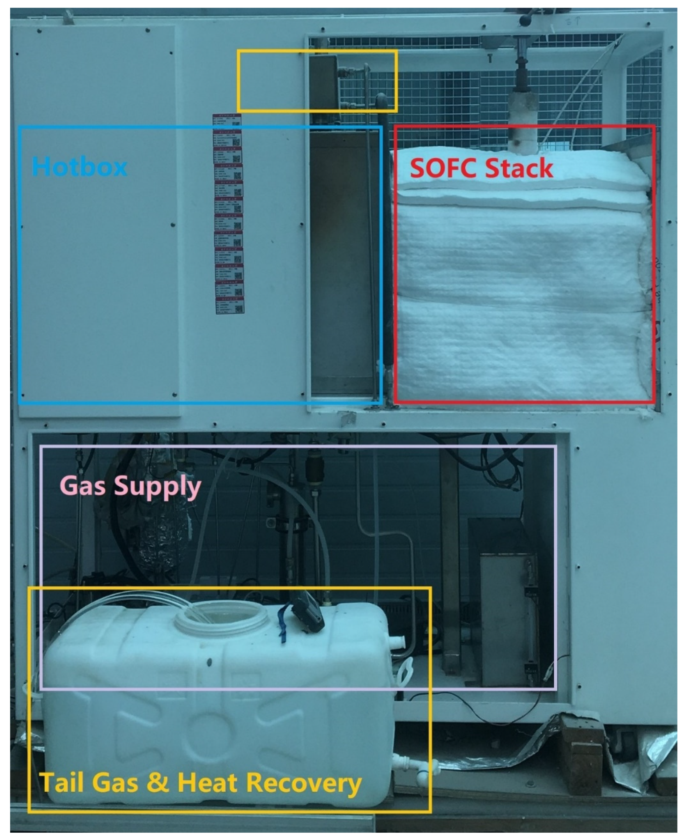
2.1. System Structure

This experiment uses a 1 kW SOFC power generation system from the Fuel Cell R&D Center of Huazhong University of Science and Technology [34]. As shown in Figure 1, the hotbox includes high-temperature components such as heat exchangers, reformers, and combustion chambers. The cold box includes low-temperature components such as water tanks, desulfurizers, blowers, etc. The fuel selection for SOFC power generation systems is characterized by diversity. In this experiment methane was used, which is also relevant for the following BOP components. A general SOFC system must have a BOP component in addition to the most critical stack. The SOFC stack is composed of multiple single-cell stacks, and the BOP components mainly include the reformer, heat exchanger, exhaust burner, blower, air-storage tank, and water-cooling tank, as shown in Figure 2. The following electrochemical reactions occur in the single cell to convert chemical energy into electrical energy.

$${\mathrm{H}}_2+1/2{\mathrm{O}}_2\to {\mathrm{H}}_2\mathrm{O}+\mathrm{heat}+\mathrm{electricity}$$

(1)

$$\mathrm{CO}+1/2{\mathrm{O}}_2\to {\mathrm{CO}}_2+\mathrm{heat}+\mathrm{electricity}$$

(2)

The stack used in this experiment consists of 27 cells. Each cell has an area of $15\times 15 {\mathrm{cm}}^2$, and the effective working area is $13\times 13{ \mathrm{cm}}^2$. The reactants are natural gas at 99.5% methane concentration and deionized water. It is worth mentioning that the reformer used in this experiment consists of a reformer chamber and burner chamber. The former is used to generate hydrogen from the reforming reaction and the latter is used to heat the methane combustion, so no external heat source is required. The water-to-carbon ratio of the system was limited to 1.5~3.0. Too low of a ratio will lead to carbon deposition, and too high will lead to unstable thermoelectric properties. At this ratio, hydrogen production was most efficient. The workflow of the whole system is as follows:

In the fuel channel, the natural gas is divided into two parts. One part of the methane gas is desulfurized and mixed with deionized water to enter the reforming chamber for the reforming reaction. The other part of the gas is mixed with air and burned directly in the combustion chamber to generate heat to raise the temperature of the reforming chamber, which facilitates the positive reforming reaction. The gas from the reforming reaction is preheated by a co-flow heat exchanger and then enters the SOFC stack anode.

In the air channel, the air supplied by the blower enters the reactor cathode after preheating by the cross-flow heat exchanger and after the co-flow heat exchanger. The inlet temperature difference between the cathode (air) and the anode (fuel) of the stack is the difference in gas inlet temperature, which can cause deformation and rupture inside the stack. Among them, the co-flow heat exchanger is set to reduce the temperature difference of the inlet gas of the stack and ensure the safety of the temperature gradient of the stack.

The electrochemical reaction takes place inside the stack, converting chemical energy into electricity and heat. The exhaust gas produced by the reaction exists with a certain amount of flammable gas, which is mixed and burned in the combustion chamber to release heat and raise the temperature of the burner while reducing the emission of the harmful gas carbon monoxide. The high-temperature exhaust from the burner preheats the air in the heat exchanger. The preheated air is thermally balanced with the fuel gas to heat the fuel gas to 500–600 °C, thus improving the operating efficiency of the system.

2.2. Experimental Scheme and Data Analysis

From several SOFC system experiments, the one with the highest output power was selected as the subject of this paper. The start-up of the SOFC system is a slow process. In the early stages of startup, the electrochemical reactions cannot take place because the temperature has not reached the required range and therefore no electricity can be output. The incoming fuel gas all reaches the combustion chamber directly to generate heat, and then uses the heat exchanger to heat the air and fuel gas, thus preheating the stack. When the temperature of the reactor rises to within the range where electrochemical reaction occurs and stabilizes, the system’s connected electrical load is turned on so that the system current begins to rise. The system power generation process can be divided into the current-rise phase, the high-temperature zero-current phase, and the long-term stable operation phase, based on the change in current, some of which occur more than once during the experiment. Due to the relatively poor dynamic ability of the SOFC system to respond, when there is a suddenly increasing load, the SOFC system cannot supply enough fuel and generate enough heat in time to maintain operation under the new load conditions. Big changes in operating conditions can also seriously affect the normal running and life cycle of the BOP component [35]. The load should be gradually increased during the current rise phase to make the current rise smoothly and slowly to avoid the problem of a fuel deficit. The electrical characteristics of the SOFC system during the entire experiment with time are shown in Figure 3. During the first current rising phase, the current rose to 8 A. The voltage did not decrease significantly during this period, indicating that the fuel supply to the system was sufficient at this time. While the current continued to rise to 26 A, there was an obvious fall in the output voltage curve, indicating that the stack was in a state of slight fuel deficit. Next, the SOFC system went into a hot standby mode, at which time the current was 0 A, the voltage rose to open-circuit voltage, and the output power was zero, but the stack temperature was still at a higher value, i.e., the high-temperature zero-current stage. After the end of the hot standby state, the second current-rise phase started, with the current rising to 55 A. A load test was conducted with the current gradually climbing to a peak of 75 A when the power also reached maximum. Finally, it entered long-term stable operation and the current returned to 53 A. At this stage, the whole system was in self-heating equilibrium, but the current showed a decreasing trend, indicating that the stack was in the degradation period. From Figure 3, it can be seen that after reaching the power peak back down, there was a large degradation of the reactor performance.

During the experiment, 629,873 sets of SOFC system operation data were collected with a sampling time of 1 s. Each set of data was an 82-dimensional row vector, i.e., 82 features. The 82 features included both features of the SOFC stack and features of the BOP components. Among them, the key features (pressure, temperature) of the SOFC stack and BOP components as well as the gas-supply curves are presented in Figure 4. These features can be divided into two categories, one for Boolean variables and one for numerical variables. Numerical variables mainly include voltage, current, gas flow rate, pressure, temperature, etc. Boolean variables mainly include solenoid valve switches, flow valve switches, and so on. Since an SOFC system is a power generation device, the most important concern is its pure output power. The power is calculated from the voltage and current. In the electrical characteristics of the SOFC output, one variable is usually controlled to observe the decay of the other variable. The stack studied in this paper belongs to the current type, i.e., the current is the independent variable according to the external load demand, whereas the voltage value belongs to the corresponding dependent variable, so the main concern is the trend of the voltage value of the stack under the system. The state of the SOFC stack can only be observed indirectly by observing the voltage variation, so voltage is one of the most important and typical state variables. The indicator of stack failure is that the stack voltage is less than 70% of the rated voltage. Therefore, when the predicted voltage is less than 70% of the rated voltage, the stack is deemed to have failed.

In the short-term degradation experiments, there were some problems and phenomena with unclear mechanisms:

• There was high-frequency dithering at 150,000–300,000 s at the anode inlet temperature of the stack (Figure 4b);
• The reconditioner temperature fluctuated slightly throughout the whole operation (Figure 4c);
• There was a sudden, significant drop in the heat-exchanger cathode inlet temperature after 600,000 s, with gas supply not changing significantly and only gas pressure fluctuating (Figure 4c);
• There was a steep rise and fall in the temperature of the exhaust combustion chamber with a high frequency of jitter in the inlet temperature values between 100,000 and 300,000 s (Figure 4c).

These phenomena are difficult to explain mechanistically, so they are collectively referred to as thermoelectric dithering phenomena. These phenomena cannot be represented by mechanistic modeling, so a data-driven approach is needed to complement the SOFC system operating characteristics. Meanwhile, it can be seen in Figure 3 and Figure 4a that the flow rate of the reactant gas was highly correlated with the thermoelectric characteristics of the SOFC system, proving that the input gas was the main cause of the system state change.

3. Prognostic Method for the Degradation of the SOFC System

In this section, the basic principles and characteristics of two RNN morphs—long short-term memory (LSTM) [36] and gated recurrent network (GRU) [37]—will be introduced first. Then we will explain how the attention mechanism works and combine it with two deep learning models, LSTM and GRU, in order to build a prediction model based on the encoder–decoder mechanism. In the end, the implementation steps of the prognostic model and the processing of the raw dataset, including feature selection, data filtering, and so on, are introduced.

3.1. Neural Network

3.1.1. Recurrent Neural Network

A recurrent neural network (RNN) is a neural network with memory capability. Therefore, it has good results in processing sequence data and has wide applications in the fields of natural language processing [38] and sentiment analysis [39]. The basic structure of RNN has an input layer, a hidden layer, and an output layer, which are basically the same as a normal neural network. Unlike normal neurons, its hidden layer has an arrow pointing to itself, indicating the passing of data updates. This is the reason why RNNs have the ability to memorize. As shown in Figure 4a, the hidden layer state at each moment is determined by both the input at the current moment and the hidden layer state at the previous moment. The state of the hidden layer is updated by the following equation:

$$h=f\left(h_{t-1},x_t\right)$$

(3)

where $x_t$ is the input at the current moment, and $h_{t-1}$ is the hidden layer state at the previous moment.

Expanding the above Equation (3) can be written as:

$$h_t=f\left(w_{hh}{h}_{t-1}+w_{xh}{x}_t+b\right)$$

(4)

where $w_{hh}$ is the weight matrix from the hidden layer to the hidden layer, $w_{xh}$ is the weight matrix from the input layer to the hidden layer, $b$ is the bias vector, and $f$ is the activation function. The output expression is:

$${\widehat{y}}_t=w_{hy}{h}_t$$

(5)

where $w_{hy}$ is the weight matrix from the hidden layer to the output layer.

Because of the chain connection structure of RNN, it is able to uncover the temporal association in the data, so it has a good effect on processing time-series data. However, when a sequence is long enough, RNN suffers from short-term memory and it is difficult to retain the earlier information to the current moment. It is also called the long-term dependencies question. Two specific manifestations of the long-term dependencies question in practical training are gradient explosion [40] and gradient vanishing [41]. To solve the long-term dependence problem of RNN, two RNN-based neural networks (LSTM and GRU) are proposed. In this paper, these two gated RNNs are used to predict the change in the output voltage state of the SOFC system.

3.1.2. Long Short-Term Memory

LSTM is a particular variant of an RNN network that can learn and utilize long-term dependent information. The structure of LSTM is shown in Figure 5b, and its external connections are not very different from RNN. However, there is a big change inside the LSTM hidden layer with the addition of a gate control mechanism and cell states. The cell state of the LSTM, which controls the transmission of temporal information, is the key to the absence of the long-term dependencies question in the LSTM. The output of the forgetting gate determines the proportion of the cell state from the previous moment that can be retained until the current moment. The input gate determines the percentage of the current moment’s input in the new cell state. The output gate outputs a portion of the updated cell state.

Therefore, the working steps of LSTM can be divided into the following three steps. First, the forget gate retains the cell state associated with the current moment. Then, the input gate adds some of the inputs of the current moment to the cell state to complete the cell-state update. Finally, the output gate retains part of the cell state as the output of the hidden layer. The working mechanism of the three gates can be summarized by the following equation:

$$f_t=\sigma \left(W_f·\left[h_{t-1},x_t\right]+b_f\right)$$

(6)

$$i_t=\sigma \left(W_i·\left[h_{t-1},x_t\right]+b_i\right)$$

(7)

$$o_t=\sigma \left(W_o·\left[h_{t-1},x_t\right]+b_o\right)$$

(8)

where $\left[h_{t-1},x_t\right]$ is the vector connection between the hidden layer state and the current input at the previous moment; $W_f$, $W_i$, and $W_o$ are the weight matrices between the connection vector and the output of each gate; and $b_f$, $b_i$, and $b_o$ are the bias matrices of the three gates.

The update of the cell state and the output of the hidden layer are calculated as follows:

$${\tilde{c}}_t=tanh(W_c·\left[h_{t-1},x_t\right]+b_c)$$

(9)

$$c_t=f_t\ast c_{t-1}+i_t\ast {\tilde{c}}_t$$

(10)

$$h_t=o_t\ast tanh(c_t)$$

(11)

LSTM avoids the problem of gradient explosion and gradient disappearance due to long-term dependence by gating the unwanted information and retaining the information related to the current state due to the setting of the cell state and gating mechanism. Therefore, LSTM has very good results for tasks that require long-term memory. However, it is also the introduction of the gating mechanism that leads to more neural network parameters and makes the training more difficult.

3.1.3. Gated Recurrent Unit

GRU is also a kind of deformation of RNN, which is also proposed to ameliorate the long-term dependency problem of RNN. Compared with LSTM, it has a simpler structure and faster training speed. The structure of GRU is shown in Figure 5c, which combines an input gate and an oblivion gate into an update gate. The function of the update gate is to determine the percentage of information to be passed from the past to the future, or what is called update memory. Another gate of GRU is the reset gate, used to choose how much of the past hidden layer state to ignore. The expressions for these two gates are:

$$z_t=\sigma \left(W_z·\left[h_{t-1},x_t\right]+b_z\right)$$

(12)

$$r_t=\sigma \left(W_r·\left[h_{t-1},x_t\right]+b_r\right)$$

(13)

The state update expression for the hidden layer is:

$${\tilde{h}}_t=tanh(W_h·\left[r_t\ast h_{t-1},x_t\right]+b_h)$$

(14)

$$h_t=\left(1-z_t\right)\ast h_{t-1}+z_t\ast {\tilde{h}}_t$$

(15)

where $W_z$, $W_r$, and $W_h$ are the weight parameter matrices between the layers; $z_t$ is the output of the update gate; $r_t$ is the output of the reset gate; $h_t$ is the hidden state at time t; and $b_z$, $b_r$, and $b_h$ are bias matrices.

3.2. RNN-Based Encoder–Decoder

In this paper, the prediction of the output time-series data from the input time-series data is a typical structure of Seq2Seq. The Seq2Seq structure contains an encoder and a decoder. The encoder can parse the information from the input data, obtain the features in the data, and convert them into a form that is conducive to machine learning for the purpose of accelerated learning. The decoder is tasked with using the higher-order, abstract information obtained by the encoder to predict the sequence output.

In this paper, the encoder–decoder RNN model is used, where the RNN used is LSTM or GRU. The encoder–decoder RNN contains two identical RNN models, located in the encoder and decoder, respectively, and its structure is shown in Figure 6 below. The encoder is a one-way RNN without an output, responsible for reading the input sequence and encoding it as a fixed-length vector—the background variable $c$, where the hidden state at each moment depends only on the input subsequence before the current time. The state transformation formula of the hidden layer is

$$h_t=f\left(x_t,h_{t-1}\right)$$

(16)

where $x_t$ is the input of the current time step and $h_{t-1}$ is the hidden state of the previous time step.

Transformation of the hidden state of each time step into background variables is carried out by means of the custom function q:

$$c=q\left(h_1,\cdots ,h_T\right)$$

(17)

where T is the max time step.

For example, when choosing $q\left(h_1,\cdots ,h_T\right)=h_T$, the background variable is the hidden state of the final time step of the input sequence. In this paper, the q used is the LSTM or GRU network.

The RNN in the decoder is responsible for mapping the background variables into a variable-length output sequence. At the current time step $t’$, the input to the decoder is the output $y_{t’-1}$ at the previous moment with the background variable $c$, and it converts them with the hidden state $s_{t’-1}$ at the last time step to the new hidden layer state $s_{t’}$ at the current time, which can be expressed by the following equation:

$$s_t=f\left(s_{t-1},y_{t-1},c\right)$$

(18)

where $s_t$ is the hidden state and $y_{t-1}$ is the input of the previous time step.

Finally, the output prediction of the model can be calculated:

$$P\left(y_T|y_{t-1},y_{t-2},y_1,c\right)=g\left(s_t,y_{t-1},c\right)$$

(19)

where $y_T$ is the output at time step T.

3.3. Data Processing

In this paper, the raw observation data from the SOFC system experiment was a 629,873 × 82-dimensional data set with a sampling time of 1 s. The characteristics of SOFC systems can be divided into electrical characteristics and thermal characteristics. The electrical characteristics change quickly, in units of seconds. The thermal characteristics change more slowly, in minutes. Therefore, in order to observe the changes in thermoelectric properties of the whole SOFC system more visually, the data need to be compressed and the redundant data need to be removed. From the original dataset, every 60 rows, a record is picked and put into a new dataset. This results in a new dataset with a sampling time of 1 min and a size of 10,323 × 82. After compressing the rows, compression is also performed for the columns. The 82 features in the original data would make the neural network too complex, increasing the computational cost and training time. First, the Boolean variables from the 82 features are removed, which are typically switch signals. The remaining 72 features have a large number of repetitive temperature features with similar trends and features that can be computed from other features. Based on experimental experience and literature review, 18 features were retained out of 72 features, as shown in

Table 1. Selected features of the SOFC system.

	Features
Output voltage	Cathode air pressure	Reformer temperature
Output current	Bypass air pressure	Anode inlet temperature
Cathode air-flow rate	Anode input pressure	Cathode inlet temperature
Bypass air-flow rate	Cathode input pressure	Anode outlet temperature
Methane flow rate	Anode output pressure	Cathode outlet temperature
Input methane pressure	Cathode output pressure	Burner temperature

below. The size of the dataset was reduced to 10,323 × 18.

The size of the dataset was greatly reduced after filtering, but 18 features was still too much, so sequential forward selection (SFS) was used for the further feature selection. SFS is a bottom-up approach. The first feature selects the feature that is individually optimal and has the best prediction effect. The second feature is the feature that works best in combination with the first feature from the remaining special features, and so on to obtain the combination of features that works best. Finally, a combination of features consisting of four features was determined, which were output voltage, output current, input methane pressure, and cathode air pressure. Their changes with time are shown in Figure 7.

After the data are filtered, the data need to be normalized to avoid the influence of different magnitudes and orders of magnitude on the evaluation index, and to accelerate the learning speed of the neural network and improve the prediction accuracy. In this paper, linear normalization is used, and its calculation formula is shown as follows:

$$x_{norm}=\frac{x-x_{min}}{x_{max}-x_{min}}$$

(20)

where $x_{norm}$ is the data after deflation, $x$ is the original data, $x_{max}$ is the maximum value, and $x_{min}$ is the minimum value.

After the data normalization is completed, the structure of the data needs to be reorganized. Since time-series data cannot be used directly for training models, they need to be converted to supervised learning data before they can be used for training. Sliding time windows were used to divide the data into input and output data at fixed time steps, as shown in Figure 8. Doing so increased the size of the training set. As an example, we input the state for the first 10 min and predicted the state for the next 10 min. Next, the time window was moved back one minute and the states from 1–11 min were entered to predict the states from 11–21 min, and so on.

3.4. Prognostic Method Framework

Based on the above discussion, the framework of the RNN prediction method based on the encoder–decoder mechanism established in this paper is shown in Figure 9. The detailed steps of the prediction model are as follows:

• Raw data from short-term degradation experiments of SOFC systems were collected and pre-processed, including data culling, feature selection, normalization, etc.
• For the processed data, the first 7500 min were used as the training set and the last 7500 min as the test set, where 20% of the training set was randomly selected as the validation set.
• The relevant parameters for the encoder–decoder LSTM/GRU were selected. Since there were four features, the input layer had four nodes and the number of nodes in the hidden layer was set to 32. There was a fully connected layer of 10 nodes between the hidden layer and the output layer. Finally, since the output of the model was a stack voltage, the output layer had only 1 node.
• The relevant training hyperparameters were determined, including time step, batch size, and epoch.
• The optimizer and loss function for the model were selected, the model was trained using the training set, the predicted voltage of the test set was compared with the true value, and the result was evaluated.

4. Results and Discussion

In this section, the SOFC experimental data from Section 2 are used to train the deep learning-based prediction model built in Section 3. Four different prediction models, LSTM, encoder–decoder LSTM, GRU, and encoder–decoder GRU are used to forecast the voltage state changes of the SOFC system and analyze the prediction results.

4.1. Evaluation Criteria

In order to measure the prediction results, the corresponding indexes must be used to evaluate the degree of fit of the results to the real data. In this paper, three criteria—mean square error (MSE), mean absolute error (MAE), and coefficient of determination (R²)—are used to evaluate the prediction results. The closer the value of MSE and MAE is to 0, the smaller the error between the prediction result and the true value, and the closer the predicted value is to the true value. The normal range of R² is [0, 1], and the larger it is, the better the model fits the data. The correlation formula is as follows:

$$\mathrm{MSE}=\frac{{\sum }_{i=1}^N{(y_i-{\widehat{y}}_i)}^2}{N}$$

(21)

$$\mathrm{MAE}=\frac{{\sum }_{i=1}^N\left|y_i-{\widehat{y}}_i\right|}{N}$$

(22)

$${\mathrm{R}}^2=1-\frac{{\sum }_{i=1}^N{(y_i-{\widehat{y}}_i)}^2}{{\sum }_{i=1}^N{(y_i-{\overline{y}}_i)}^2}$$

(23)

where $y_i$ is the true measured value of the SOFC output voltage, ${\overline{y}}_i$ is the average of the real voltage data, ${\widehat{y}}_i$ is the prognostic voltage, and $N$ is the overall number of true output voltages.

4.2. Results of the LSTM-Based Model

In this subsection, LSTM and encoder-decoder LSTM prediction models are constructed. The model is trained and the voltage variation of the SOFC is predicted using the processed dataset. The inputs of the model are output voltage, output current, input methane pressure, and cathode air pressure, and the output is voltage. The hyperparameters of the hidden layers are particularly critical for the neural network model. A larger number of hidden layers and nodes will lead to an overly complex model, which will greatly increase the model training time; a smaller number will lead to a degradation of the model prediction performance and fail to achieve the expected results. In this paper, based on the relevant experience, we initially selected the parameter range of hidden layers, and then used the grid-search method to search the optimal parameters. The number of LSTM layers was two and the number of nodes was 32. In addition to the hidden layer parameters, time step is also an important parameter that affects the prediction performance. The time step was set to 10, i.e., the data from the first 10 min were used to predict the data from the second 10 min.

After model construction and parameter selection, the prognostic outcomes of the processed dataset were calculated. The prognostic results of the original LSTM model are shown in Figure 10. The data set was divided into two parts around 7500 min, where (0, 7500) min is the training set and (7500, 10,000) min is the test set. From Figure 10a, it can be found that the prediction curves of both the training and test sets fit the original data well, but the prediction of the training set was slightly better than that of the test set, which proves that the model had no overfitting problem. At several peak points, the voltage mutation was too fast and the prediction effect needed to be enhanced. From Figure 10b, it can be found that the prediction model converged very quickly in the training process, experiencing a total of 20 epochs, having converged at around the ninth epoch. The error of the validation set was slightly lower than that of the training set at the beginning, and it was higher than that of the training set afterwards, which also indicates that the model was not overfitted. In general, the LSTM-based prediction model had good performance in predicting the SOFC output voltage.

Based on the above prediction model, it was changed to the encoder–decoder LSTM prediction model, and the number of nodes of LSTM in the encoder and decoder was kept the same. After the construction, the model was applied to the dataset for prediction, and the prediction results are shown in Figure 11. In Figure 11a, it can be seen the prediction curve of the new model was smoother and fit the original curve more closely than the previous model. The evaluation results of the two models are shown in

Table 2. Calculation of the evaluation criteria for prediction results.

	Training Set				Test Set
	LSTM	Encoder–Decoder LSTM	GRU	Encoder–Decoder GRU	LSTM	Encoder–Decoder LSTM	GRU	Encoder–Decoder GRU
MSE	0.013956	0.011820	0.013129	0.011521	0.017050	0.014966	0.017456	0.015121
MAE	0.082145	0.059687	0.078887	0.057455	0.094432	0.084220	0.097976	0.086195
R2	0.963418	0.981198	0.964254	0.982704	0.936420	0.964618	0.933110	0.961665

. In the training phase, the MSE of the LSTM mode was 0.013956 and the MSE of the encoder–decoder LSTM mode was 0.011820. In the testing phase, the MSE of the LSTM mode was 0.016550 and the MSE of the encoder–decoder LSTM mode was 0.015121. These data demonstrate that the new model was more accurate than the original LSTM model. The R² of the new model was 0.981198 in the training phase and 0.964618 in the testing phase, which shows that the proposed model fit the dataset better. During the experiment, the presence of some faults (heat-exchanger rupture, reformer-reforming performance degradation, and exhaust combustion chamber airflow imbalance) led to sudden voltage changes and spikes. However, it can be seen in Figure 10a and Figure 11a that the model still had some prediction capability for abrupt voltage changes, and these abnormal states could be partially fitted to the model.

4.3. Results of the GRU-Based Model

From the previous section, it can be seen that encoder–decoder LSTM had better prediction performance compared to the original LSTM. To verify the role of encoder–decoder RNN architecture network, in this section, the GRU-based prediction model and the encoder–decoder GRU prediction model is constructed to repeat the prediction task to verify the effectiveness of the encoder–decoder mechanism. After the grid search, the hyperparameters of the GRU model were determined as 32 nodes with two layers. The prediction results are presented in Figure 12. From Figure 12a, it can be seen that the first half of the prediction curve of the training set fit well with the original data. Comparing Figure 10a,b, the prediction curve of the GRU model was shifted downward compared with the original curve, but the number of epochs required for GRU to converge was smaller. This was due to the characteristics of GRU, which sacrifices the prediction performance (number of parameters inside the hidden layer) to improve the training speed.

Next, the performance of the encoder–decoder GRU was observed in a real-world application, and its prediction results are shown in Figure 13. The prognostic performance of the new model was enhanced when measured against the GRU model. This can be seen visually from the comparison of Figure 12a and Figure 13a, where the encoder–decoder GRU model had a more stable output, and its prediction curve was more consistent with the original data and less volatile. Comparing Figure 12a with Figure 13a, it can be found that the validation set error was smaller and converged faster after adding the encoder–decoder. From the perspective of evaluation metrics, the MSE of the new model was 0.011521 and 0.014966 in the training phase and testing phase, respectively, which are lower than before, indicating that the new model predicted more accurately.

The MAE, MSE, and R² of the four models were all calculated with the training set data and the test set data, so they had the same reference standard. The smaller the MAE and MSE, the smaller the average error at each min. The MAE and MSE of the LSTM and GRU models did not differ significantly, indicating that the difference between the prediction accuracy of these two models was little. The R² of both was also similar, indicating that the prediction results of both were similar to the true value fitting level. Theoretically, when the LSTM and GRU have the same number of neurons, the LSTM network will have more internal parameters, and therefore the prediction is a little bit better. The GRU network, on the other hand, had slightly fewer parameters and trained a little faster. This can also be seen in Table 2, where the MAE and MSE of GRU were larger and the R² was smaller. After adding the encoder–decoder mechanism, the new models were more capable of information extraction, processing, and prediction of data, and MAE and MSE were decreased and the R² was increased.

5. Conclusions

In this paper, a new data-driven deep learning fuel cell-state prediction model is proposed. Recurrent neural networks (RNN) with long short-term memory (LSTM) units and gated recurrent units (GRU) are used as the encoder and decoder to avoid the gradient-vanishing and gradient-exploding problem in network training. Short-term degradation experiments of the SOFC system were designed to collect raw data. The model prediction results are validated by the output voltage profile of the system. In addition, different degradation models, including ordinary LSTM and GRU networks, are compared with the proposed encoder–decoder model. The following conclusions can be drawn:

• The results show that the proposed encoder–decoder model can effectively achieve high prediction accuracy under realistic fuel cell operating conditions. Encoder–decoder LSTM and encoder–decoder GRU RNN models had RMSE errors (test phase) of 0.015121 and 0.014966, respectively, whereas the LSTM and GRU models had corresponding values of 0.017050 and 0.017456, which proves that the encoder–decoder RNN had higher performance.
• The proposed model still had some predictive tracking ability for large changes in the data. When the training data changed less, the prediction model had better and more reliable performance compared to the existing work.
• The proposed model can be tested for predictive performance by varying the sliding time step as well as the number of input sequences to suit different SOFC systems and even different fuel cell systems.

The model can be used to predict the fuel cell lifetime and also help monitor the operational performance of fuel cells in real applications. Due to its simple structure, the proposed RNN-based encoder–decoder prediction model is easy to implement once it has been trained. In the future, the model can be further developed to combine with PHM technology to help improve the durability of SOFC systems and even other fuel cells by making joint decisions with existing control strategies.

References

1. Revankar, S.; Majumdar, P. Fuel Cells: Principles, Design, and Analysis; CRC Press: Boca Raton, FL, USA, 2014; ISBN 9781420089684. [Google Scholar]
2. Damo, U.M.; Ferrari, M.L.; Turan, A.; Massardo, A.F. Solid Oxide Fuel Cell Hybrid System: A Detailed Review of an Environmentally Clean and Efficient Source of Energy. Energy 2019, 168, 235–246. [Google Scholar]
3. Wu, X.L.; Xu, Y.W.; Xue, T.; Shuai, J.; Jiang, J.; Deng, Z.; Fu, X.; Li, X. Control-Oriented Fault Detection of Solid Oxide Fuel Cell System Unknown Input on Fuel Supply. Asian J. Control 2019, 21, 1824–1835. [Google Scholar]
4. Xu, H.; Ma, J.; Tan, P.; Chen, B.; Wu, Z.; Zhang, Y.; Wang, H.; Xuan, J.; Ni, M. Towards Online Optimisation of Solid Oxide Fuel Cell Performance: Combining Deep Learning with Multi-Physics Simulation. Energy AI 2020, 1, 100003. [Google Scholar] [CrossRef]
5. Bello, I.T.; Zhai, S.; Zhao, S.; Li, Z.; Yu, N.; Ni, M. Scientometric Review of Proton-Conducting Solid Oxide Fuel Cells. Int. J. Hydrog. Energy 2021, 46, 37406–37428. [Google Scholar] [CrossRef]
6. Faheem, H.H.; Abbas, S.Z.; Tabish, A.N.; Fan, L.; Maqbool, F. A Review on Mathematical Modelling of Direct Internal Reforming- Solid Oxide Fuel Cells. J. Power Sources 2022, 520, 230857. [Google Scholar]
7. Yuan, Z.; Wang, W.; Wang, H.; Ghadimi, N. Probabilistic Decomposition-Based Security Constrained Transmission Expansion Planning Incorporating Distributed Series Reactor. IET Gener. Transm. Distrib. 2020, 14, 3478–3487. [Google Scholar] [CrossRef]
8. Huang, Y.; Turan, A. Fuel Sensitivity and Parametric Optimization of SOFC—GT Hybrid System Operational Characteristics. Therm. Sci. Eng. Prog. 2019, 14, 100407. [Google Scholar] [CrossRef]
9. Yang, W.J.; Park, S.K.; Kim, T.S.; Kim, J.H.; Sohn, J.L.; Ro, S.T. Design Performance Analysis of Pressurized Solid Oxide Fuel Cell/Gas Turbine Hybrid Systems Considering Temperature Constraints. J. Power Sources 2006, 160, 462–473. [Google Scholar] [CrossRef]
10. Hou, Q.; Zhao, H.; Yang, X. Economic Performance Study of the Integrated MR-SOFC-CCHP System. Energy 2019, 166, 236–245. [Google Scholar] [CrossRef]
11. Zio, E. Prognostics and Health Management (PHM): Where Are We and Where Do We (Need to) Go in Theory and Practice. Reliab. Eng. Syst. Saf. 2022, 218, 108119. [Google Scholar] [CrossRef]
12. Zhang, D.; Cadet, C.; Yousfi-Steiner, N.; Druart, F.; Bérenguer, C. PHM-Oriented Degradation Indicators for Batteries and Fuel Cells. Fuel Cells 2017, 17, 268–276. [Google Scholar] [CrossRef]
13. Barelli, L.; Barluzzi, E.; Bidini, G. Diagnosis Methodology and Technique for Solid Oxide Fuel Cells: A Review. Int. J. Hydrog. Energy 2013, 38, 5060–5074. [Google Scholar] [CrossRef]
14. Lanzini, A.; Madi, H.; Chiodo, V.; Papurello, D.; Maisano, S.; Santarelli, M.; van Herle, J. Dealing with Fuel Contaminants in Biogas-Fed Solid Oxide Fuel Cell (SOFC) and Molten Carbonate Fuel Cell (MCFC) Plants: Degradation of Catalytic and Electro-Catalytic Active Surfaces and Related Gas Purification Methods. Prog. Energy Combust. Sci. 2017, 61, 150–188. [Google Scholar] [CrossRef] [Green Version]
15. Kuramoto, K.; Hosokai, S.; Matsuoka, K.; Ishiyama, T.; Kishimoto, H.; Yamaji, K. Degradation Behaviors of SOFC Due to Chemical Interaction between Ni-YSZ Anode and Trace Gaseous Impurities in Coal Syngas. Fuel Processing Technol. 2017, 160, 8–18. [Google Scholar] [CrossRef]
16. Papurello, D.; Lanzini, A. SOFC Single Cells Fed by Biogas: Experimental Tests with Trace Contaminants. Waste Manag. 2018, 72, 306–312. [Google Scholar] [CrossRef]
17. Parhizkar, T.; Hafeznezami, S. Degradation Based Operational Optimization Model to Improve the Productivity of Energy Systems, Case Study: Solid Oxide Fuel Cell Stacks. Energy Convers. Manag. 2018, 158, 81–91. [Google Scholar] [CrossRef]
18. Tariq, F.; Ruiz-Trejo, E.; Bertei, A.; Boldrin, P.; Brandon, N.P. Chapter 5—Microstructural Degradation: Mechanisms, Quantification, Modeling and Design Strategies to Enhance the Durability of Solid Oxide Fuel Cell Electrodes. In Solid Oxide Fuel Cell Lifetime and Reliability; Brandon, N.P., Ruiz-Trejo, E., Boldrin, P., Eds.; Academic Press: Cambridge, MA, USA, 2017; pp. 79–99. ISBN 978-0-08-101102-7. [Google Scholar]
19. Laurencin, J.; Delette, G.; Lefebvre-Joud, F.; Dupeux, M. A Numerical Tool to Estimate SOFC Mechanical Degradation: Case of the Planar Cell Configuration. J. Eur. Ceram. Soc. 2008, 28, 1857–1869. [Google Scholar] [CrossRef]
20. Peng, J.; Huang, J.; Wu, X.L.; Xu, Y.W.; Chen, H.; Li, X. Solid Oxide Fuel Cell (SOFC) Performance Evaluation, Fault Diagnosis and Health Control: A Review. J. Power Sources 2021, 505, 230058. [Google Scholar] [CrossRef]
21. Silva, R.E.; Gouriveau, R.; Jemeï, S.; Hissel, D.; Boulon, L.; Agbossou, K.; Yousfi Steiner, N. Proton Exchange Membrane Fuel Cell Degradation Prediction Based on Adaptive Neuro-Fuzzy Inference Systems. Int. J. Hydrogen Energy 2014, 39, 11128–11144. [Google Scholar] [CrossRef]
22. Javed, K.; Gouriveau, R.; Zerhouni, N.; Hissel, D. Prognostics of Proton Exchange Membrane Fuel Cells Stack Using an Ensemble of Constraints Based Connectionist Networks. J. Power Sources 2016, 324, 745–757. [Google Scholar] [CrossRef]
23. Morando, S.; Jemei, S.; Hissel, D.; Gouriveau, R.; Zerhouni, N. Proton Exchange Membrane Fuel Cell Ageing Forecasting Algorithm Based on Echo State Network. Int. J. Hydrogen Energy 2017, 42, 1472–1480. [Google Scholar] [CrossRef]
24. Liu, H.; Chen, J.; Hou, M.; Shao, Z.; Su, H. Data-Based Short-Term Prognostics for Proton Exchange Membrane Fuel Cells. Int. J. Hydrog. Energy 2017, 42, 20791–20808. [Google Scholar] [CrossRef]
25. Liu, H.; Chen, J.; Zhu, C.; Su, H.; Hou, M. Prognostics of Proton Exchange Membrane Fuel Cells Using a Model-Based Method. IFAC-PapersOnLine 2017, 50, 4757–4762. [Google Scholar] [CrossRef]
26. Zhou, D.; Al-Durra, A.; Zhang, K.; Ravey, A.; Gao, F. Online Remaining Useful Lifetime Prediction of Proton Exchange Membrane Fuel Cells Using a Novel Robust Methodology. J. Power Sources 2018, 399, 314–328. [Google Scholar] [CrossRef]
27. Jiang, H.; Xu, L.; Struchtrup, H.; Li, J.; Gan, Q.; Xu, X.; Hu, Z.; Ouyang, M. Modeling of Fuel Cell Cold Start and Dimension Reduction Simplification Method. J. Electrochem. Soc. 2020, 167, 044501. [Google Scholar] [CrossRef]
28. Shao, Y.; Xu, L.; Zhao, X.; Li, J.; Hu, Z.; Fang, C.; Hu, J.; Guo, D.; Ouyang, M. Comparison of Self-Humidification Effect on Polymer Electrolyte Membrane Fuel Cell with Anodic and Cathodic Exhaust Gas Recirculation. Int. J. Hydrogen Energy 2020, 45, 3108–3122. [Google Scholar] [CrossRef]
29. Arriagada, J.; Olausson, P.; Selimovic, A. Artificial Neural Network Simulator for SOFC Performance Prediction. J. Power Sources 2002, 112, 54–60. [Google Scholar] [CrossRef]
30. Wu, X.L.; Xu, Y.W.; Xue, T.; Zhao, D.Q.; Jiang, J.; Deng, Z.; Fu, X.; Li, X. Health State Prediction and Analysis of SOFC System Based on the Data-Driven Entire Stage Experiment. Appl. Energy 2019, 248, 126–140. [Google Scholar] [CrossRef]
31. Song, S.; Xiong, X.; Wu, X.; Xue, Z. Modeling the SOFC by BP Neural Network Algorithm. Int. J. Hydrogen Energy 2021, 46, 20065–20077. [Google Scholar] [CrossRef]
32. Wu, X.; Ye, Q.; Wang, J. A Hybrid Prognostic Model Applied to SOFC Prognostics. Int. J. Hydrogen Energy 2017, 42, 25008–25020. [Google Scholar] [CrossRef]
33. Dolenc, B.; Boškoski, P.; Stepančič, M.; Pohjoranta, A. Juričić State of Health Estimation and Remaining Useful Life Prediction of Solid Oxide Fuel Cell Stack. Energy Convers. Manag. 2017, 148, 993–1002. [Google Scholar] [CrossRef]
34. Zheng, Y.; Wu, X.L.; Zhao, D.; Xu, Y.W.; Wang, B.; Zu, Y.; Li, D.; Jiang, J.; Jiang, C.; Fu, X.; et al. Data-Driven Fault Diagnosis Method for the Safe and Stable Operation of Solid Oxide Fuel Cells System. J. Power Sources 2021, 490, 229561. [Google Scholar] [CrossRef]
35. Zhang, L.; Jiang, J.; Cheng, H.; Deng, Z.; Li, X. Control Strategy for Power Management, Efficiency-Optimization and Operating-Safety of a 5-KW Solid Oxide Fuel Cell System. Electrochim. Acta 2015, 177, 237–249. [Google Scholar] [CrossRef]
36. Hochreiter, S.; Schmidhuber, J. Long Short-Term Memory. Neural Comput. 1997, 9, 1735–1780. [Google Scholar] [CrossRef]
37. Cho, K.; van Merriënboer, B.; Gulcehre, C.; Bahdanau, D.; Bougares, F.; Schwenk, H.; Bengio, Y. Learning Phrase Representations Using RNN Encoder-Decoder for Statistical Machine Translation. In Proceedings of the EMNLP 2014: Conference on Empirical Methods in Natural Language Processing, Doha, Qatar, 25–29 October 2014; pp. 1724–1734. [Google Scholar] [CrossRef]
38. Xie, H.; Anuaruddin, M.; Ahmadon, B.; Yamaguchi, S. Evaluation of Rough Sets Data Preprocessing on Context-Driven Semantic Analysis with RNN. In Proceedings of the 2018 IEEE 7th Global Conference on Consumer Electronics (GCCE), Nara, Japan, 9–12 October 2018. [Google Scholar]
39. Pola, S.; Sheela Rani Chetty, M. Behavioral Therapy Using Conversational Chatbot for Depression Treatment Using Advanced RNN and Pretrained Word Embeddings. Mater. Today Proc. 2021, in press. [Google Scholar] [CrossRef]
40. Pascanu, R.; Mikolov, T.; Bengio, Y. Understanding the Exploding Gradient Problem. arXiv 2012, arXiv:1211.5063. [Google Scholar]
41. Hochreiter, S. The Vanishing Gradient Problem during Learning Recurrent Neural Nets and Problem Solutions. Int. J. Uncertain. Fuzziness Knowl. Based Syst. 1998, 6, 107–116. [Google Scholar] [CrossRef] [Green Version]
Figure 1. 1 kW SOFC power generation system.
Energies 15 06294 g001
Figure 2. SOFC system structure.
Energies 15 06294 g002
Figure 3. SOFC system voltage-current curve.
Energies 15 06294 g003
Figure 4. Experimental response curve of the SOFC system in full working condition. (a) SOFC system gas-supply curve; (b) SOFC stack operating parameter curve; (c) BOP component parameter variation curves.
Energies 15 06294 g004aEnergies 15 06294 g004b
Figure 5. (a) Architecture of RNN; (b) schematic diagram of LSTM; (c) schematic diagram of GRU.
Energies 15 06294 g005
Figure 6. Structure of the RNN-based encoder–decoder.
Energies 15 06294 g006
Figure 7. Selected feature change curves of the SOFC system.
Energies 15 06294 g007
Figure 8. Sliding time window.
Energies 15 06294 g008
Figure 9. Structure of the encoder–decoder RNN model.
Energies 15 06294 g009
Figure 10. Prediction results of original LSTM model. (a) Model training and prognosis results; (b) training loss during the training phase.
Energies 15 06294 g010
Figure 11. Prediction results of the encoder–decoder LSTM model. (a) Model training and prognosis results; (b) training-phase loss.
Energies 15 06294 g011
Figure 12. Prediction results of the original GRU model. (a) Model training and prognosis results; (b) training loss during the training phase.
Energies 15 06294 g012
Figure 13. Prediction results of the encoder–decoder GRU model. (a) Model training and prognosis results; (b) training-phase loss.
Energies 15 06294 g013