Estimation of Underground MV Network Failure Types by Applying Machine Learning Methods to Indirect Observations

Abstract

Electrical utilities performance is measured by various indicators, of which the most important are very dependent on the interruption time after a failure in the network has occurred, such as SAIDI. Therefore, they are constantly looking for new techniques to decrease the fault location and repair times. A possibility to innovate in this field is to estimate the failed network component when a fault occurs. This paper presents the conclusion of an analysis carried out by the authors with the aim to estimate failure types of underground MV networks based on observable indirect variables. The variables needed to carry out the analysis must be available shortly after the failure occurrence, which is facilitated by a smart-grid infrastructure, to allow for a quick estimation. This paper uses the groundwork already carried out by the authors on ambient variables, historical variables, and disturbance recordings to design an estimator to predict between four MV cable network failure types. The paper presents relevant analyses on the design and performance of various machine learning classification algorithms for estimation of the types of MV cable network failures using real-world data. Optimization of performance was carried out, resulting in an estimator with an overall 68% accuracy rate. Accuracy rates of 94% for cable failure, 63% for excavations, and 79% secondary busbar failures were achieved; as for cable joints, the accuracy was poor due to the difficulty to identify a feature that can be used to separate this failure type from cable failures. Future work to improve that accuracy is discussed.

1. Introduction

The amount and variety of data readily available to electric power utilities has been increasing with the advent of smart grids, as older systems are replaced by newer ones. Furthermore, fast communication technology is accessible at low cost in substations and for MV network sensors, which enables the near real-time retrieval of data that can be used for complex analysis, which is useful from a practical perspective.

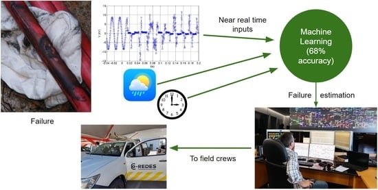
One of the main targets of electrical utilities is to provide the best quality of service possible to their clients while striving to minimize costs. Therefore, they are continuously innovating and testing new ways to achieve these goals. The larger part of interruption times that most clients experience is mostly due to outages arising from faults in the MV network. Although electrical utilities already have in place various forms of fault location methods (mainly based on impedance methods and fault passage indicators), which facilitate the job of the field crews by narrowing the search area, there is still room to improve on the type and amount of useful information that can be provided in near-real time. If, in addition to the fault location zone, information is already being provided, it is also possible to provide an estimate of the failed equipment and of the failure type, which would be a benefit for day-to-day operations of field crews. It is the expectation of the authors that that information brings about operational gains, as it will facilitate finding the failed equipment and will provide information to better prepare for the repair, consequently leading to a decrease in the overall interruption duration.

The research presented by the authors focuses on methods intended to estimate the probability of each type of failure in an underground MV network immediately after it has occurred. Providing the estimated probability for each failure type would help the teams in occurrences where the most probable cause has a probability similar to that of another cause. This should be considered during the location and repair process. To that end, the authors propose using oscillography records readily available from protection units’ or power quality analyzers as well as calendar data and weather data. The intended goal of the authors work is depicted in Figure 1.

Estimation of failures has been applied using artificial intelligence, notably in the field of machine fault diagnostics through electrical measurements [1] and acoustic measurements [2]. Industry interest in this field has motivated researchers to develop and evaluate new methods for fault diagnostics and then to other fields such as wind turbines [3] and transformers [4].

In an earlier work by the authors, the relationships between several ambient variables and the occurrence of the most common four types of failures in the Portuguese MV cable network were presented [5]. It was shown that failures caused by excavations are very dependent on date and time; both secondary substation failures and related excavations display a significant relationship with daily rainfall and dew point vs. ambient temperature; and accumulated rainfall and average temperature display a relationship with cable failures.

In addition to weather variables, oscillographic fault records provide valuable information for building a failure type estimator. This subject has been studied by an IEEE working group [6]. The resulting report details the expected fault, typically resulting from ageing, signatures for cables, overhead lines, transformers, switches, capacitor banks, surge arrestors, and potential transformers. A generic method for waveform abnormality detection is proposed in [7], based on the comparison of statistical distributions of waveform variations with and without disturbances and the difference obtained by means of a Kullback–Leibler divergence. In [8], it was shown that recurrent fault conditions are relevant for utilities and on-line automated methods to mine, cluster, and report recurrent faults to utility operators in a near-real-time fashion. The detection of incipient faults is also the subject of [9], in which they demonstrate the corresponding relationship to permanent faults. This paper’s authors have carried out an analysis on the waveform characteristics most common in failures occurring in the Portuguese MV cable network [10], which are related to ageing but also to external factors.

Usage of machine learning methods to classify fault events was the subject of [11,12], which were applied to faults occurring in overhead lines and were mainly based on the waveform analysis (although [11] also considers seasonality and hour of the day).

The authors’ aim is to develop an optimal machine learning classification method to estimate the failure type of a recently occurred fault with only indirect variables such as oscillography data and weather data. To that end, Section 2 provides a brief explanation of the machine learning classification process together with several choices pertaining to the validation process. Then, each classification method assessed for performance is presented. The dataset is detailed in the following section as well as the features used for classification algorithm. Results of each estimator’s performance are presented in Section 3, and a feature selection optimization is carried out. Probability estimation using the supervised learning algorithm with the best performance is addressed together with the corresponding results. Finally, Section 4 contains a discussion on the results, and in Section 5, the conclusions are drawn.

To the authors’ knowledge, failure estimation has never been applied to underground MV network failures, constituting a new subject in literature and requiring several new studies to ascertain the best features. It is the authors’ aim to provide a first contribution in this field.

This paper uses data from 369 real-world failures with known failure types occurring in the Portuguese underground MV network. Cable networks in Portugal display many similarities to MV underground cable networks in other parts of the world. However, the reader must consider that local factors may lead the failure types to present different relationships with the indirect variables considered in this paper.

The authors of this study expect that by presenting novel research that is not frequently seen in the literature, it will offer both academic researchers and practicing engineers useful information.

2. Materials and Methods

2.1. Classification Supervised Learning

This paper aims at estimating a class of failure and classifying it given a set of indirect observations. There is available a large set of real cases and the indirect observations to train machine learning algorithms; therefore, it a supervised learning problem.

Figure 2 displays the typical process of designing and testing a classification estimator. There is a set of samples with known results (training set) that are used to train the classification algorithm and determine the parameters α (Figure 2) that achieve the best classification result. Then, new instances are classified according to the trained algorithm. Parameters α depend on the algorithm as well.

When the classification algorithm is trained, it is necessary to assess its performance. Using the same data for training and testing can lead to a phenomenon known as overfitting [13]. If such an event occurs, the classifier can display a small error (or none) when applied to the training data but not to new data. Overfitting can indicate that the underlying physical phenomenon is not well-characterized by the algorithm, and another one should be assessed. Cross-validation was developed to assess the performance of trained algorithms without being misled by overfitting. It consists of training the classification algorithm with holding apart k samples of the available data and then assessing the classification error for the k samples (test set). The process is repeated until all samples have been tested. The overall algorithm performance is assessed by considering the accuracy of the estimation on all samples. In this paper, k = 2 samples were used for the cross-validation. The variable k refers to the number of instances left out in the cross-validation process. If k is larger, more instances are not being used for the training process, which results in a lower computational load. However, the training process benefits from a large training set, as it better adjusts the classification algorithm to the data, thus resulting in a higher accuracy. After a trial-and-error process, the authors concluded that k = 2 had an acceptable processing time and allowed for the use of most of the available instances for training, thus resulting in a better estimate of a real working estimator.

2.2. Classification Algorithms

There are several types of classification algorithms, ranging from simple ones such as nearest neighbor (kNN) to more complex ones such as support vector machines (SVM). They use different methods to solve the classification problem. These are generic methods that can be used for a variety of classification problems. Each classification problem has an intrinsic model, which, most of the time, is unknown. Therefore, it is not previously known in a real-world situation which method will be more adapted to classify the instances. Therefore, it is usual to test various classification algorithms to determine which one is more suitable for the given real-world problem.

Of the classification methods presented, SVM and boosting are considered as usually displaying the best accuracy. SVM has a more computationally heavy training stage but a simple estimation stage, while boosting is usually not so computationally demanding on the training stage but more demanding on the estimation phase. However, with the present computational power, no methods display a computational limitation.

Next, several commonly used classification algorithms are presented.

2.2.1. Support Vector Machines (SVM)

Support vector machines is a linear classifier. Its purpose is to define a hyperplane that minimizes the linear classifier risk bound [14,15]. The classifier risk is the expected misclassification error. The classifier risk itself cannot usually be determined, but an upper and lower bound can be. The upper bound of a linear classifier depends on a variable named margin, which depends on the training data.

SVM’s training algorithms use optimization methods to maximize the margin for the given data within the training set. Classification is simple because SVM is a linear classifier. Equation (1) is used for classification in binary linear classifiers.

$$y={\beta }_0+{\beta }^{T}x$$

(1)

The sign of y will determine the estimated class (binary classifier). The training process will determine β and β₀ from the training data.

Previously, it has been shown that SVM is a “state of the art” linear classifier. However, linear classifiers have a limited scope of application. Efforts have been carried out to overcome this limitation, which led to the appearance of kernel functions [16]. These functions are used to map the training data into a different space, which can re-arrange the data in such a way that a linear classifier presents a better performance. However, the usage of mapping functions increases problem’s dimensionality, leading to a higher computational effort at the training stage. Kernel functions display several properties that minimize the added computational cost.

2.2.2. Boosting Algorithms

Boosting algorithms use other classification algorithms that have a poor performance (marginally better than 50% accuracy rate for the binary problem), i.e., “weak learners” [17]. It can be a one-layer tree, “stump”, or other types of simple classifiers.

The output function of any boosting algorithm is a weighted linear combination of many “weak learners” (2). For the binary case, the sign of the output refers to the estimated class.

$$H\left(x\right)=sign\left({\displaystyle \sum }_{t=1}^T{\alpha }_t{h}_t\left(x\right)\right)$$

(2)

where α_t is the weight of the “weak learner” function, $h_t\left(x\right)$ is the “weak learner” function, and T is the number of “weak learners” being used.

Training of boosting algorithms consist of determining the weights of the output function. There are various algorithms and variants of algorithms to determine these weights. The most famous are: AdaBoost [18], LPBoost [19], RUSBoost [20], and TotalBoost [21]. Some of them are easily computed, while others are less prone to overfitting, and their performance is less susceptible to outliers.

Boosting algorithms are computationally less demanding for large dimension training sets, thus minimizing the “curse of dimensionality” issue that affects most classifier’s training, and their performance is regarded typically as being good.

2.2.3. K Nearest Neighbors (kNN)

“Nearest neighbor” is one of the simplest classification algorithms and the only one used in this paper that does not require training.

The classification algorithm consists of determining a distance (usually a Euclidian distance) between the feature vector of the class that we wish to estimate and every entry in the training data and then choosing the k samples in the training set that display the lowest distance. The class is estimated by the number samples of the training set that are nearer to the feature vector whose class is being estimated.

Selection of the number of samples nearer to the sample that we intend to classify is an issue. If the number k is too small, then there is a danger of underfitting, and if it is too high, then the overfitting is a problem. There is rule of thumb that k should be close to the square root of the amount of data in the training set [22].

If certain conditions are met (large number of samples in the training set and an optimally selected k), then the risk of using this method is close to the one presented by the Bayes risk (the lowest error presented by any classifier) [23].

2.2.4. Fisher Discriminant

The discriminant analysis is one of the earliest types of classification algorithms. It was developed by Ronald Fisher in 1936 and has since then undergone some improvements. There is a good description of the method in [24].

Discriminant analysis is performed under the assumption that all classes follow a Gaussian distribution. The mean and covariance matrix for each class is determined numerically from the training set.

Classification is carried out by determining the estimated probability of each class given the new sample and selecting the class that displays the highest probability.

2.2.5. Decision Trees

Decision trees are widely used for classification (e.g., in biology by classifying all species of animals). It aims to provide an estimate for the classification by following several “if” rules applied to the data (e.g., if age <2 and if age >1, then it is a toddler). These rules can grow in depth (a tree of rules) and reach high levels of complexity.

Training of decision trees is usually carried out by the “top-down induction of decision trees” algorithm [25], which defines the rules given a training set of data.

Classification is carried out by following the set of rules established during the training stage.

2.2.6. Bagging Algorithms

Bagging, or bootstrap aggregating, is a meta-algorithm that aims at improving the accuracy of other learning algorithms. It is usually used in conjunction with decision trees.

Given the training set, the bagging algorithm establishes several smaller training sets. It then fills the smaller training sets by sampling randomly and with replacement from the original training set. It then uses a learning algorithm (e.g., decision trees) to determine several classifiers, one for each subset of training set data [26].

Classification is carried out by voting using the estimate of the classifier output for each of the training subsets.

2.2.7. Subspace Algorithms

This technique is intended to create a classifier based on decision trees that retains the maximum accuracy of training data and increases generalization accuracy as the classifier becomes more sophisticated [27]. The classifier consists of several trees built systematically by pseudo-randomly choosing subsets of feature vector components, or trees, built in randomly selected subspaces.

2.3. Data and Features

A dataset of 369 of real failures in the Portuguese underground MV network was obtained for training and assessing the performance of classification algorithms. The main failure types of the underground cable network in Portugal and their frequency of occurrence over a 14-year period, in which over 6000 underground cable failures were observed, were presented in [5]. The 369-instance dataset was selected to match to the 14-year period failure type frequency to achieve the most realistic performance results. The fault types, relative percentages, and number of instances in the dataset are:

• Class 1—Cable insulation failures (57%, 210 instances);
• Class 2—Excavation damages (11%, 41 instances);
• Class 3—Secondary substation (SS) busbar failures (9%, 33 instances);
• Class 4—Cable joint failure (23%, 85 instances).

It is the aim of this paper to build an estimator that can classify each instance with the previous four classes of failures. To that end, the following features, which were derived in [5,11] and extracted from each occurrence, were considered:

• Feature 1—Fault type (e.g., single line to ground);
• Feature 2—Evolving fault (binary);
• Feature 3—Number of self-clearing faults;
• Feature 4—Relation between the maximum voltage and the voltage at which the fault occurred;
• Feature 5—Fault occurring during normal a working period;
• Feature 6—Electric arc voltage;
• Feature 7—Number of intra-cycle self-clearing faults;
• Feature 8—Voltage before insulation breakdown in intracycle self-cleared faults;
• Feature 9—Voltage difference between intracycle pre-breakdown voltage and voltage after breakdown;
• Feature 10—Day average temperature minus dew point;
• Feature 11—Rainy day (binary);
• Feature 12—30-day mean temperature.

Features 5, 10, 11 and 12 are obtained either by calendar or by meteorological data and are relatively straightforward. The remaining features are determined by carrying out a signal processing of the oscillography records. Details for the signal processing are not presented in this paper due to its complexity, but a detailed explanation on the extraction of each feature can be found in [10]. An example of the observed frequency of Feature 1 (fault type) is presented in Figure 3; however, the depiction of all features would be a lengthy exercise and would not bring any new development relative to [10]. The features are used in all the assessments in this paper and will be referenced by their number for simplicity reasons.

Although there was a considerable number of failures in the Portuguese underground network in 14-year period, not all substations were equipped with disturbance recording in this period. Some relied on protection relays for disturbance recording, and some of them only stored a small number of records (around 6), which meant that data were lost if not retrieved quickly. Despite these challenges, a dataset of 369 known failures was obtained and is large enough to assess estimator performance.

3. Results

3.1. Initial Results

The 369 occurrences were used to train fourteen classification algorithms and assess their accuracy using a twofold cross-validation and a “one vs. one” method for binary classifiers. MATLAB Statistics and Machine Learning toolbox functions were used to train and assess the various algorithms. The results are presented in

Table 1. Results of the accuracy performance assessment of various classification algorithms with the 369 occurrences.

Classification Algorithm	Accuracy
Tree	61.5%
Linear Discriminant	64.8%
Naïve Bayes	52.3%
SVM (linear)	65.9%
SVM (quadratic)	61.5%
SVM (cubic)	58.8%
SVM (Gaussian)	66.4%
kNN (Euclidean distance)	64.8%
kNN (cosine distance)	63.4%
kNN (cubic distance)	63.4%
AdaBoost	64.0%
Bagging	62.9%
Subspace discriminant	65.0%
RUSBoost	53.7%

.

The best-performing classification estimator is the Gaussian kernel SVM, which displays an accuracy rate of 66.4%. A question then arises: is this performance good?

The goodness of the accuracy of a given estimator depends on the end use. In this case, it is intended to have the best accuracy possible. However, the comparison must also be made with the best information available at present. The simplest estimator is to choose the most likely failure class, which is cable insulation failure, for all occurrences. Given this assumption, the resulting accuracy would be 57% [5]. Hence, 66.4% is higher than 57%, which means that the Gaussian kernel SVM estimator provides more accurate information than the best available estimator to date.

Accuracy is only part of the information concerning the performance of estimator. The ability to correctly predict each of the classes is also important. This assessment is carried out by means of a confusion matrix (Figure 4). In this approach, the matrix is built in such a way that the predicted class and true class are matched, and each instance added to the correct combination of true and predicted class. This allows to determine the estimator performance for each class.

The Gaussian kernel SVM displays a very good performance on predicting class 1 (cable insulation failure, 94.8%), class 2 (excavation damage, 53.7%), and class 3 (secondary substation busbar failure, 69.7%). However, for class 4 (cable joint failure), the accuracy is only 1.2%, and most instances were classified as cable insulation failure (95.3%). This result means that the features being used cannot adequately separate cable joint failures from cable insulation failures.

Another common analysis on the performance of estimators is the ROC curve (receiver operating characteristic curve), which illustrates the diagnostic ability of a binary classifier system, as its discrimination threshold is varied. In this analysis, the best estimators display a larger AUC area. Classifier performance in an “one vs. all” perspective is presented in brackets.

The ROC curves of Figure 5 also indicate that the classifier performance is good in determining classes 1 (cable insulation failure), 2 (excavation damage), and 3 (SS busbar failures) while presenting a poor performance on class 4 (cable joint failure).

3.2. Feature Selection

When dealing with a relatively high number of features, it is possible that some of them are redundant because there are others that convey the same information or irrelevant because their correlation with the class may be low [28]. This issue should be taken into account while designing classification algorithms as [29] shows.

Using more features than necessary leads to added numerical complexity of the training and class estimation process. It may also lead to overfitting of the classification algorithm, thus reducing the accuracy of the classifier.

Several techniques have been developed to deal with this issue [28]. Nonlinear optimization algorithms, such as genetic algorithms, are typically used to carry out feature selection. All of them are intended to select the features that yield the best success rate (determined using cross-validation) while minimizing the number of features.

This paper considers twelve features to carry out the classification performance assessment, which is a relatively small number, and due to its low dimension, determining the best features is possible by using an exhaustive search within an acceptable time. After carrying out an exhaustive search, it was determined that the classifiers display the best accuracy if features 7 (self-clearing faults under a one-fourth cycle) and 12 (mean 30-day ambient temperature) are removed.

Table 2. Results of the accuracy performance assessment of various classification algorithms with the 369 occurrences after discarding features 7 (evolving fault) and 12 (mean 30-day ambient temperature).

Classification Algorithm	Accuracy
Tree	65.0%
Linear Discriminant	66.7%
Naïve Bayes	62.3%
SVM (linear)	68.0%
SVM (quadratic)	67.8%
SVM (cubic)	67.8%
SVM (Gaussian)	66.9%
kNN (Euclidean distance)	65.6%
kNN (cosine distance)	65.6%
kNN (cubic distance)	65.0%
AdaBoost	67.2%
Bagging	66.1%
Subspace discriminant	66.1%
RUSBoost	53.7%

displays the performance of every classification algorithm using the remaining ten features.

By comparing Table 1 and Table 2, the performance of all classification algorithms improved slightly except for RUSBoost, which remained the same. The best classification estimator performance increased to 68% from 66.4%.

The confusion matrix displayed in Figure 6 shows that although there was a slight decrease in the number of correctly predicted instances for class 1 (cable insulation failure—198 instances correctly predicted, 94.2% accuracy), it improved the correctly predicted classes 2 (excavation related failures—26 instances correctly predicted, 63.4% accuracy) and 3 (secondary substation busbar failures—26 instances correctly predicted, 78,8% accuracy), with the overall performance increasing. However, there is no change to the performance of the correctly predicted cable joint failures, which remains negligible. This confirms the earlier conclusion that the features used in this paper do not display the necessary information to separate cable insulation failures from joint failures.

ROC curves also display an increased performance by removing the two features (Figure 7), as the AUC areas are slightly larger in all comparisons.

Overall, there is a minor performance increase by removing the two features from the estimator conception. This also leads to a less computationally demanding process.

It should be stated that these classification algorithms’ performance was determined using real data from the Portuguese MV cable network and that other utilities may display a different relative frequency for failures (e.g., excavation cable damage may be more frequent). In this case, the overall performance may be different as well as the relative frequency of the most common class, which serves as a reference for the assessment.

3.3. Estimating Probabilities from Classification Algorithms

Estimating the probability of the classification result being correct is not straightforward and depends on the classification algorithm being used. The algorithm that presented the best accuracy was the SVM (linear or with the Gaussian kernel); therefore, this analysis will focus on estimating the probability of the SVM algorithm being correct.

A good method for estimating the probability is described in [30]. It uses a sigmoid function to approximate the probability of the classification being correct (3).

$$P(y=1|\widehat{y})=\frac{1}{1+e^{A\widehat{y}+B}}$$

(3)

In (3), $\widehat{y}$ is obtained by (1); however, A and B need to be calculated by an iterative method for each instance. The process used is described in [30].

After applying the previously described method to the linear SVM, classifier data for the feature selection results in probabilities for each of the four classes for all the 369 instances. Due to conciseness issues, the option was to present the data aggregated in the form of histograms. Figure 8 displays the percentages that were estimated when the linear SVM classification algorithm was successful.

Most commonly, the estimated probability of the estimator being correct is 65% to 75% when it is successful. However, larger and smaller values are also observed. The incorrect class with the largest probability is usually on the 25% to 30% range.

Figure 9 displays the estimated probability when the SVM linear algorithm fails and selects the wrong class. In this, although the wrong class presents mainly percentages in the 65% to 75% range, no wrong class was observed with a percentage above 85%. The correct classes present estimated probabilities mainly in the 25% to 30% range. This is due to the difficulty of separating the cable insulation failure events from the cable joint events, as was already demonstrated previously by the analysis of Figure 6.

4. Discussion

This paper’s analysis was carried out using real data from the Portuguese cable MV distribution network. The amount of available data allows for confidence that the results will hold in a real-life application. The results have shown that a feature selection process has yielded positive results and should be carried out in similar applications.

The classification algorithms employed have proven to provide a more accurate information (accuracy rate of 66%) than an estimator that selects only the most common class (accuracy rate of 57%). The feature selection process improved this accuracy even further to 68%.

Even with the feature selection process, the results have shown that cable insulation and cable joint failures were not adequately separated by the estimator. There was a tendency to group both failure types under the cable insulation failure type, which is not surprising because it is the most numerous classes. The features set does not possess sufficient information to separate both classes. The authors have investigated the information present in the oscillography records but did not identify any features present that may have helped to distinguish between the two failure types. From a visual point of view, both failures wave forms are similar. The sequence of failure types in a feeder and at the substation was also investigated, but it did not yield the information required for a separation of both failure types.

Separating the estimation of cable insulation failures from joint failures seems difficult. The authors believe that it is possible to achieve better results by obtaining fault oscillography with a higher sampling rate (the highest sampling rate used was of 254 samples/s), which may show the presence of high harmonic signals; however, the capacitor nature of cables may strongly attenuate those signals. Another possibility includes obtaining the information of the technician who built the joint and the age of the joint and corresponding cables. The authors did not have access to this type of information and therefore were not able to carry out an analysis with those data.

In other countries with other types of MV network, soil characteristics, and challenges, there might be some changes to some of these results. Therefore, it is advisable to carry out a similar analysis to the one presented in this paper before starting to build an estimator.

5. Conclusions

In this paper, it has been shown that:

• Machine learning classification can provide better information (68% accuracy) than just simply considering all occurrences as belonging to the most common class (57% accuracy).
• This performance is achieved by using calendar data, meteorological data, and oscillography data to train a linear SVM algorithm. All these data can be readily available for processing, and the whole estimation can be carried out in near-real time, which could provide valuable information for field crews tasked with finding and fixing the failure.
• It was also found that the fourteen features and also the twelve features after the features selection process considered in the analysis did not have sufficient information to adequately distinguish between cable joint failures and cable insulation failures. Because cable insulation failures are more common in the dataset (which was selected to represent the overall failure type frequency in the Portuguese cable network), 93% of cable insulation failures were incorrectly estimated to be a cable insulation failure.
• The classification algorithms were able to distinguish between the other three classes with a good performance (94.2% for cable insulation failure, 63.4% for excavation damages, and 78.8% for SS busbar failures).
• Future improvements in the performance of the proposed estimator must rely on the identification of new features that can adequately be used to distinguish between cable insulation failures and cable joint failures.
• After carrying out a feature selection process, it was found that classification algorithms displayed a slightly better performance by removing feature 7 (self-clearing faults under a one-fourth cycle) and feature 12 (mean 30-day ambient temperature). Therefore, the estimation algorithm displays a better performance with a lower computational cost of signal processing in the oscillography records, in training the classifier, and in predicting the class for every new instance.

The original contribution of this paper is that it has shown that it is possible to distinguish between several types of cable network failures with a high accuracy (68%) using only twelve features (indirect observations) and a linear SVM classifier. This can be used to improve the information available to electrical utility operations.