Abstract
This paper describes the effect of the incidence angle of the bucket on the performance of the axial turbine stage. The off-design operating conditions of the turbine stage result in a change in the velocity diagrams. This results in a positive or negative incidence. One of the basic objectives in turbine stage design is to estimate the flow behaviour of the turbine stage during off-design operation as accurately as possible and to quantify the corresponding decrease in efficiency. The available loss prediction models allow the estimation of the loss distribution when the incidence angle changes in the preliminary design phase. However, the incidence angle is actually affected by the velocity of circulation, which changes the input velocity vector (induced incidence). Thus, the blade row angle of attack is different from the angle based on the velocity diagram calculations. The result of our paper is a relation for estimating the angular difference of the input flow angle to the bucket defined as a function of the turbine operation mode.
1. Introduction
Fluid flow in turbomachinery is generally one of the most complex processes in mechanical engineering. Physical phenomena occurring in the turbomachine flow paths are dealt with by research facilities and scientific institutes all over the world. This is both in the context of experimental research, but also in the context of the numerical approach (CFD analysis) that has become increasingly popular in recent years. The great advantage of CFD simulations is the low operating cost, which only comprises the licensing fees for commercial CFD software and personnel costs. In addition, it is possible to use open source CFD codes. The outputs of CFD simulations only represent a basic outline, so it is not possible to consider these results as primarily determinative. For the credibility of the results, it is necessary to validate the numerical results by experiment. Only then can the correct conclusions be drawn. Therefore, in spite of the relatively high economic costs, experimental work should not be forgotten and should always complement CFD simulations.
Any flow path design or optimisation needs to include methods for defining flow losses (entropy generation). The source of entropy generation is viscous friction due to surface drag, heat transfer and other processes.
The total loss in the axial turbine stage consists of the sum of the partial losses such as profile losses, secondary losses, endwall losses, trailing edge losses, leakage losses, incidence losses, or other additional losses such as wetness losses, disc windage losses, etc.
2. Brief Overview of Various Loss Models
In turbomachinery practice, there are a number of mathematical models used for predicting turbine stage losses. One of the best known is the model by Ainley and Mathieson in 1951 (A&M) [1]. These authors and others have made many interesting contributions to this field. Despite the fact that these findings date back to the 1950s, they are an important source of information and remain applicable today.
Later, in 1970, there was a review of the A&M correlation by Dunham and Came (D&C) [2]. It was found that the correlations defined by A&M were not sufficient for lower power turbine stages. Modifications were made to the relationships describing secondary losses and tip leakage losses. New corrections for the Reynolds number and output Mach number were included in the D&C loss model.
In the same year, a loss model for predicting turbine stage losses by Craig and Cox (C&C) [3] was introduced. The C&C loss model could be used over a wide range of Reynolds and Mach numbers, pitch to chord ratios and other important parameters. The model included a completely new way of predicting incidence losses.
In 1981, Kacker and Okapuu (K&O) [4] introduced a loss model based on A&M correlations and a partial modification of D&C. It was shown to better predict the efficiency of a wide range of axial turbines. The main contribution of the K&O loss model was the addition of losses due to shock waves and the compressibility of the flow medium.
Later, in 1993, Denton (D) [5] presented his work in which a loss prediction methodology based on the definition of entropy increase was introduced. In terms of profile loss, according to Denton, the optimal t/c ratio and corresponding minimum profile loss can be estimated by systematically varying the estimated velocity distribution.
The problem of turbine row loss models operating in off-design operating modes has been addressed by a number of authors, such as Moustapha et al. in 1990 [6], and later by Benner et al. in 1997 [7] and Zehner in 1980 [8].
The simplest view of incidence losses is given by the Stepanov model from 1962 [9], which does not take into account the geometrical parameters of the blade row. Stepanov’s hypothesis is based on the assumption that the losses at an off-design angle of attack are proportional to the square of the vector difference between the reference (design) and non-reference (off-design) input flow velocity.
Moustapha, Kacker and Trembley (M&K&T) [6] introduced an improved methodology for predicting loss incidence based on the A&M model in 1990. The most notable change was the introduction of a new correlation parameter, namely the leading edge diameter.
Following the previous M&K&T loss model, it was further modified in 1997 by Benner, Sjolander and Moustapha (B&S&M) [7]. These authors found that the profile curvature in the transition region between the leading edge circle and the downstream part of the profile pressure and suction sides have a relatively significant effect on the profile losses due to the change in incidence angle. To account for these transient curvature changes in the profile geometry, the so-called leading edge wedge angle was introduced by the authors and included in the correlation.
In 1980, Zehner [8] presented profile losses estimation taking into account the effect of incidence. The loss coefficient is a function of the blade row geometry, flow parameters, Reynolds and Mach number.
Figure 1 compares the incidence loss models mentioned above. These dependencies correspond to the parameters of a high reaction turbine bucket with t⁄c ~0.78. From the distributions shown in Figure 1, the agreement of the incidence loss models can be seen in a narrower range of incidence angles, approximately in the range i = ±5°. In off-design regimes with higher incidence, the differences between the observed models are more pronounced.
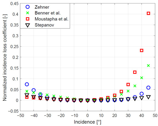
Figure 1.
Comparison of incidence loss models.
Even though the Stepanov loss model does not include any specific geometrical blade row parameters, it agrees reasonably well in the positive incidence region (up to approximately i = +30°) with a more complex Zehner model. However, at higher incidence angles, the Zehner model predicts higher incidence losses. This is due to the sensitivity of the model to the characteristics of the blade row geometry. In the negative incidence region, these two models start to diverge more significantly from approximately i = −25°.
The Moustapha and Benner loss models differ significantly from the other loss models in the positive incidence region (i > +10°). Their curves are steeper in character, with the Moustapha model predicting higher incidence losses at higher positive incidence. On the other hand, in the negative incidence region, the Benner model predicts higher losses.
The trends in the incidence loss models according to Benner and Moustapha are typical for turbine profiles with significant flow turning. The suction side is much more sensitive to the changes in incidence for these turbine profile types than the pressure side, which resists negative incidence to a greater extent. On the suction side, progressive overloading will result in much earlier flow separation.
3. Induced Incidence
From the incidence loss models described above, it is clear that the incidence angle parameter plays a key role in the loss estimation process of a blade row operating in an off-design regime. However, most available methodologies do not take into account the influence of so-called induced incidence.
Induced incidence is due to the velocity circulation around the blades. This, in addition to generating lift force, also deforms the streamlines entering the blade row. Therefore, the inlet velocity vector will attack the blade row at a different angle from that given by the velocity diagrams (see Figure 2). Figure 2 shows a profile on which the streamline is attacking with a significantly negative incidence. Due to the velocity of circulation, the inlet streamline curvature occurs near the profile, changing the inlet angle from the original value of β1f to a new (in this case smaller) value of β1f*. The actual incidence angle i* will therefore be slightly smaller than the original one.
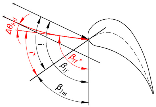
Figure 2.
Explanation of induced incidence.
In 1956, Dunavant and Erwin (D&E) [10] presented a correlation relation to estimate the induced incidence as a function of the inlet flow angle and t/c (see Figure 3). A reasonable correlation of plotted data is given by Equation (1) [11].
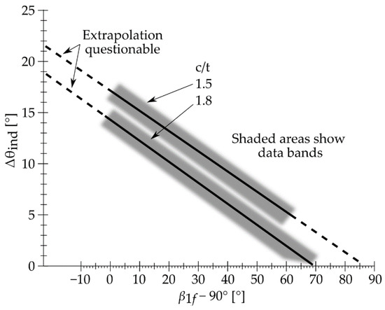
Figure 3.
Induced incidence angle by D&E. [11].
The above correlation was developed by the authors on the basis of turbine blade cascade experiments for different turbine profiles. Measurements were performed at design inlet flow angles. Measured turbine blade profiles were designed in a simple way using circles and straight lines or parabolic curves. For this reason, a new induced incidence correlation will be presented in this paper, based on an experimentally validated numerical analysis of the flow in a high reaction axial single turbine stage under off-design conditions.
4. Experimental Setup
The experimental turbine test rig (VT-400) was a 1:2 scale model of a high-pressure steam turbine part (see Figure 4). The working medium was air sucked from the atmosphere by a compressor. More detailed information about the experimental device can be found in the publication [12,13].
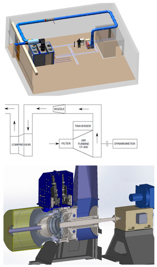
Figure 4.
VT-400 test rig. [12].
Two basic measurement tasks can be performed on the VT-400 test rig. The first task is the determination of the basic turbine stage characteristic, i.e., the dependence of the stage efficiency on the velocity ratio from torque measurement and static pressure taps. The operating mode is set by varying the stage pressure drop by controlling the compressor RPM while keeping the turbine RPM constant. Absolute speed is an isentropic velocity (or so-called spouting velocity).
The second measurement method is a detailed wake traverse measurement behind the nozzle and bucket using two five-hole pneumatic probes. In contrast to the previous measurement method, the wake traverse makes it possible to determine the radial flow distributions along the blades. In addition, this measurement method does not require torque measurement, which is associated with a relatively large measurement uncertainty.
The evaluation methodology, including the method of calibrating the pneumatic probes, is described in [12].
The basic parameters of the tested turbine stage are summarised in Table 1.

Table 1.
Geometric parameters of tested stages.
5. Numerical Simulation
Numerical simulation was performed in the commercial version of ANSYS CFX 19.3. An ideal gas was chosen as the working medium with additionally defined parameters corresponding to the conditions during the measurements. The problem was solved for a stationary turbulent flow of a viscous compressible fluid with heat transfer, the k-ω SST turbulence model and the “total energy” heat transfer model. A frozen rotor interface processing method was used in the simulation. The computational mesh, with over 50 million cells, also included bucket tip seal geometry.
The computational model of the turbine stage was halved. Thus, a half cross-section with 28 bucket blades and 29 nozzle blades was used.
The designation of the turbine stage calculation modes is included in Table 2. Mode “v2” approximately corresponds to the optimally loaded turbine. Details of the streamlines on the bucket leading edge at the mid radius for each calculated variant are shown in Figure 5.
Table 2.
Designation of calculated turbine stage modes.
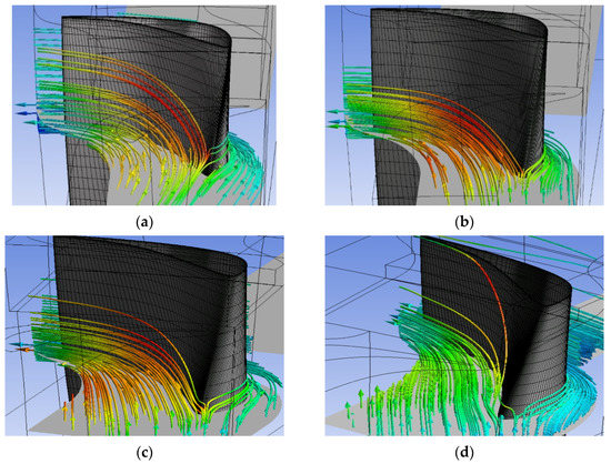
Figure 5.
Details of streamlines on the bucket leading edge at the mid radius: (a) v1; (b) v2; (c) v3; and (d) v4.
Total pressure, total temperature velocity vectors and a turbulence intensity of 5% were chosen as the boundary conditions for the numerical simulation. The quality of the computational mesh was verified using the y+ parameter. The contours of y+ on the nozzle and bucket surface are shown in Figure 6. The local maximum of y+ is approximately 1.44 for the stator blade and about 2.77 for the bucket. On most surfaces, the value of y+ is less than 1.
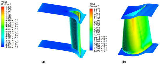
Figure 6.
Contours of the y+ parameter on: (a) nozzle; and (b) bucket.
5.1. Validation
The calculated results were compared with the experimental data to verify the numerical simulation. In the first step, the mass flow rates were compared (see Figure 7). The largest deviation of the mass flow for the nozzle is 0.9%, and for the bucket it is 1.4%.
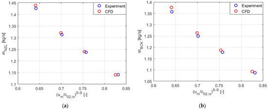
Figure 7.
Comparison of mass flow rates of: (a) nozzle; and (b) bucket.
The radial distribution of the turbine stage efficiency (T-S) is shown in the graph (Figure 8). In the hub region, a similar trend of both dependencies can be observed. However, in the blade tip region, more significant deviations between the experimental results and CFD are observed. While the experiment shows a rapid decrease in efficiency from approximately 80% of the blade length, this efficiency decrease in the CFD trend occurs at 95% of the blade length. The main reason for this deviation is due to the effect of the design holes for the movement of the pneumatic probes, which create an unstable flow field in the blade tip region. Therefore, there is a local increase in losses. Since these holes were not part of the numerical model, their influence was not included in the CFD simulation results. Another possible reason for the different efficiency values at the blade tip region is the tip leakage flow effect. The mixing of the leakage flow with the main flow significantly disturbs the flow field and creates vortex structures that greatly distort the pneumatic probe measurement results.
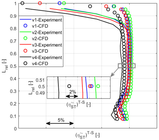
Figure 8.
Comparison of radial distributions of mass-averaged turbine stage efficiency (T-S).
Validation of CFD simulations further focused on the results of the flow angle distribution, especially the directly measured nozzle output absolute velocity angle (Figure 9 and Figure 10). The evaluation planes of the CFD simulation were identical to the measurement planes of the pneumatic probes. The radial distributions of α1f (mode “v1”) are shown in Figure 10.
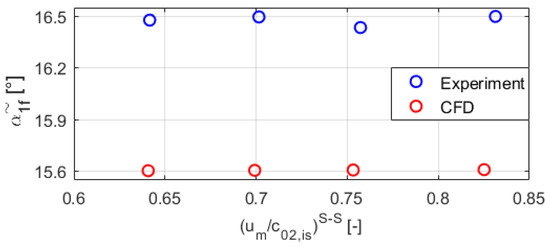
Figure 9.
Mass-averaged nozzle output absolute velocity angle at mid radius.
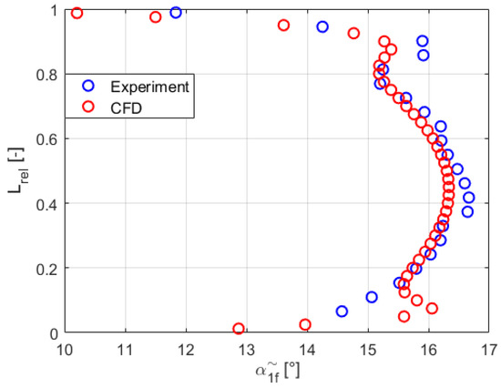
Figure 10.
Comparison of the radial distributions of mass-averaged nozzle output absolute velocity (v1).
From these dependencies, it can be concluded that the experimental results agree with the numerical simulation within acceptable limits.
5.2. Estimation of the Effective Bucket Angle of Attack
The pneumatic probe measurement behind the nozzle can only be used to measure in one plane of the axial gap between the nozzle and the bucket row. However, this means that the flow angle behind the probe changes even further and therefore the measured and actual bucket angle of attack will be different. The pressure probe measurement in this configuration cannot capture the effect of the induced incidence near the leading edge of the blade. Therefore, the results of a validated CFD analysis were used for further analysis.
The flow enters the bucket at a relative angle β1f. The following figure (Figure 11) plots the unaveraged circumferential distribution of β1f from the data of the probe measurement plane (“Beta1f_probe”) and from the data of the plane close to the bucket leading edges (“Beta1f_LE”).
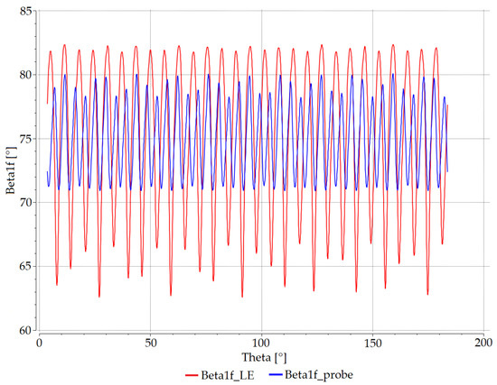
Figure 11.
Unaveraged input relative velocity angle distributions at the bucket leading edge plane and pneumatic probe plane.
The graphs (Figure 12) show the change in the mass-averaged angles β1f at the root, mid and tip blade profiles in the axial gap from the probe plane (“S”) to the bucket leading edge (“LE”). From the root profile point of view, the largest angular difference can be seen for the “v1” operating mode . For operation mode “v4”, the difference at the root profile is approximately . The mid profile also shows the largest difference for the “v1” mode, namely . In the design mode (“v2”), there is a change of . The most significant angular difference is at the bucket tip, with the largest difference in the “v3” mode (up to ). This tip region is greatly affected by the flow into the tip seal, and therefore this region was not analysed further.
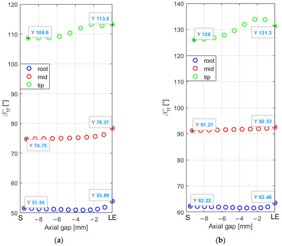
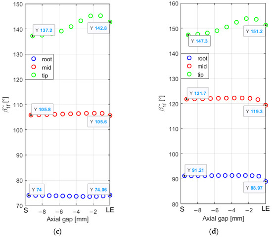
Figure 12.
Mass-averaged relative velocity angles to the bucket in the axial gap: (a) v1; (b) v2; (c) v3; and (d) v4.
The following graphs (Figure 13) show the angular differences depending on the turbine stage operating mode for the root and mid-blade profiles. A linear dependence of the angular differences is evident for the root and mid radius.
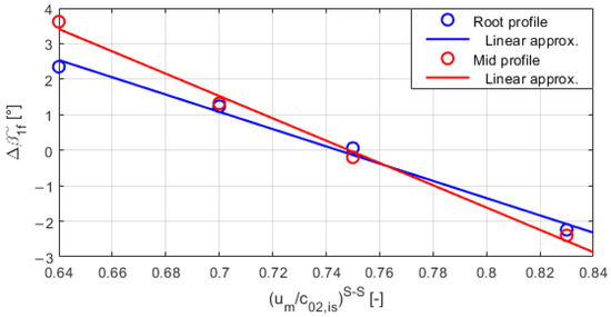
Figure 13.
Linear dependence of the angular difference at the root bucket profile.
From the obtained dependencies, it is clear that, by increasing the incidence, the angular difference will also increase. Whether this increase will be linear cannot be predicted with certainty. More measurements would be needed to obtain data over a wide range of turbine stage operating modes, and for more blade geometries.
The standard incidence loss prediction models described in the overview do not account for the effect of induced incidence. These loss models only include the standard incidence angle parameter, which should be extended to incorporate dependence: . According to the chosen orientation of the angles, the following applies to the corrected incidence angle:
For example, the incidence value for the “v1” operating mode at the mid-radius changed from the original value to . For operating mode “v4” at the same radius, the following applies: .
6. Conclusions
The circulation causes the curvature of the inlet streamlines near the leading edges of the bucket, and thus there is an angular difference between the input relative velocity vector obtained from the wake traverse and the actual vector affected by the velocity of circulation. Due to the design of the experiment, it is not possible to measure in different axial planes between the nozzle and bucket. However, the numerical simulation allows us to evaluate the flow parameters in an arbitrarily determined axial plane. Therefore, we evaluated the relative velocity angle in the axial gap between the nozzle and the bucket.
Using the results obtained from CFD analysis, we found the correlation between the angular difference of the bucket input relative velocity vector and turbine stage operating mode. This information can be useful for estimating the effective angle of attack to the bucket for the off-design operating modes of turbine stages.
Author Contributions
Conceptualisation, M.K.; Formal analysis, D.D.; Funding, P.Ž.; Project administration, P.Ž.; Software, M.K.; Validation, B.R.; Visualisation, B.R.; Writing—original draft, M.K.; Writing—review and editing, M.K. All authors have read and agreed to the published version of the manuscript.
Funding
Published with the financial support of the European Union, as part of the project entitled Development of capacities and environment for boosting the international, intersectoral and interdisciplinary cooperation at UWB, project reg. No. CZ.02.2.69/0.0/0.0/18_054/0014627 and the STUDENTSKÁ GRANTOVÁ SOUTĚŽ: SGS-2022-023 (Research and Development of Power Machines and Equipment).
Institutional Review Board Statement
Not applicable.
Informed Consent Statement
Not applicable.
Data Availability Statement
Not applicable.
Acknowledgments
This paper was written with the financial support of the European Union, as part of the project entitled Development of capacities and environment for boosting the international, intersectoral and interdisciplinary cooperation at UWB, project reg. No. CZ.02.2.69/0.0/0.0/18_054/0014627 and the STUDENTSKÁ GRANTOVÁ SOUTĚŽ: SGS-2022-023 (Research and Development of Power Machines and Equipment).
Conflicts of Interest
The authors declare no conflict of interest.
Nomenclature
| Absolute velocity, chord | ||
| Root diameter | ||
| Incidence angle | ||
| Blade length | ||
| Blade opening | ||
| Pitch | ||
| Circumferential velocity | ||
| Number of blades | ||
| Nozzle outlet absolute velocity flow angle | ||
| Bucket outlet absolute velocity flow angle | ||
| Bucket inlet relative velocity flow angle | ||
| Efficiency | ||
| Subscripts | ||
| BCK | Bucket | |
| Absolute | ||
| Design | ||
| Flow | ||
| Isentropic | ||
| LE | Leading edge | |
| m | Mid, metal (blade) | |
| NZL | Nozzle | |
| Relative | ||
| Stage | ||
| Stage input plane | ||
| 1 | Inter-stage plane | |
| 2 | Stage output plane | |
| Superscripts | ||
| Static to static | ||
| Total to static | ||
References
- Ainley, D.G.; Mathieson, G.C.R. A Method of Performance Estimation for Axial-Flow Turbines. Aeronaut. Res. Counc. Rep. Memo. 1951, 2974. Available online: https://reports.aerade.cranfield.ac.uk/handle/1826.2/3538 (accessed on 16 August 2013).
- Dunham, J.; Came, P.M. Improvements to the Ainley-Mathieson Method of Turbine Performance Prediction. J. Eng. Power 1970, 92, 252–256. [Google Scholar] [CrossRef]
- Craig, H.R.M.; Cox, H.J.A. Performance Estimation of Axial Flow Turbines. Proc. Inst. Mech. Eng. 1970, 185, 407–424. [Google Scholar] [CrossRef]
- Kacker, S.C.; Okapuu, U. A Mean Line Prediction Method for Axial Flow Turbine Efficiency. J. Eng. Power 1982, 104, 111–119. [Google Scholar] [CrossRef]
- Denton, J.D. Loss Mechanism in Turbomachines. J. Turbomach. 1993, 115, 621–656. [Google Scholar] [CrossRef]
- Moustapha, S.H.; Kacker, S.C.; Tremblay, B. An Improved Incidence Losses Prediction Method for Turbine Airfoils. J. Turbomach. 1990, 112, 267–276. [Google Scholar] [CrossRef]
- Benner, M.W.; Sjolander, S.A.; Moustapha, S.H. Influence of Leading-Edge Geometry on Profile Losses in Turbine at Off-design Incidence: Experimental Results and an Improved Correlation. J. Turbomach. 1997, 119, 193–200. [Google Scholar] [CrossRef]
- Zehner, P. Calculation of Four-Quadrant Characteristics of Turbines. In Proceedings of the International Gas Turbine Conference and Products Show, New Orleans, LO, USA, 10 March 1980. [Google Scholar]
- Stepanov, G.Y. Hydrodynamics of Turbine Cascades; Fizmatgiz: Moscow, Russia, 1962. (In Russian) [Google Scholar]
- Dunavant, J.C.; Erwin, J.R. Investigation of a Related Series of Turbine Blade Profiles in Cascade. NACA Tech. Note 3802. Available online: http://hdl.handle.net/2060/19930084558 (accessed on 16 August 2013).
- Wilson, D.G.; Korakianitis, T. The Design of High-Efficiency Turbomachinery and Gas Turbines, 2nd ed.; MIT Press: Cambridge, MA, USA, 2014; pp. 288–290. ISBN 9788120351851. [Google Scholar]
- Klimko, M.; Lenhard, R.; Žitek, P.; Kaduchová, K. Experimental Evaluation of Axial Reaction Turbine Stage Bucket Losses. Processes 2021, 9, 1816. [Google Scholar] [CrossRef]
- Klimko, M.; Okresa, D. Measurements on the VT-400 Air Turbine. Acta Polytech. 2016, 56, 118–125. [Google Scholar] [CrossRef]


Publisher’s Note: MDPI stays neutral with regard to jurisdictional claims in published maps and institutional affiliations. |
© 2022 by the authors. Licensee MDPI, Basel, Switzerland. This article is an open access article distributed under the terms and conditions of the Creative Commons Attribution (CC BY) license (https://creativecommons.org/licenses/by/4.0/).