
Design of Energy-Saving Duct for JBC to Reduce Ship Resistance by CFD Method

Abstract
:1. Introduction
2. CFD Methods
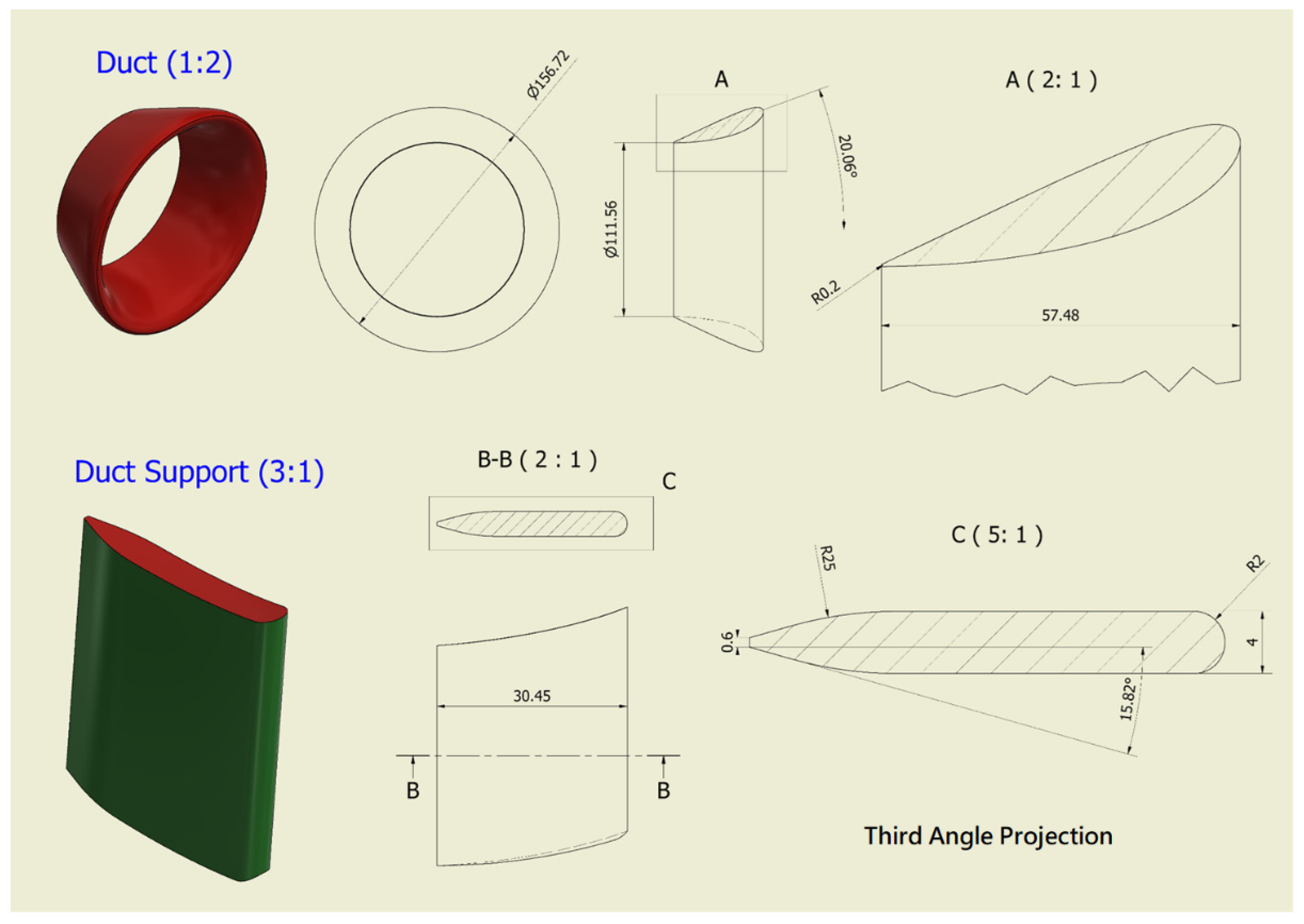
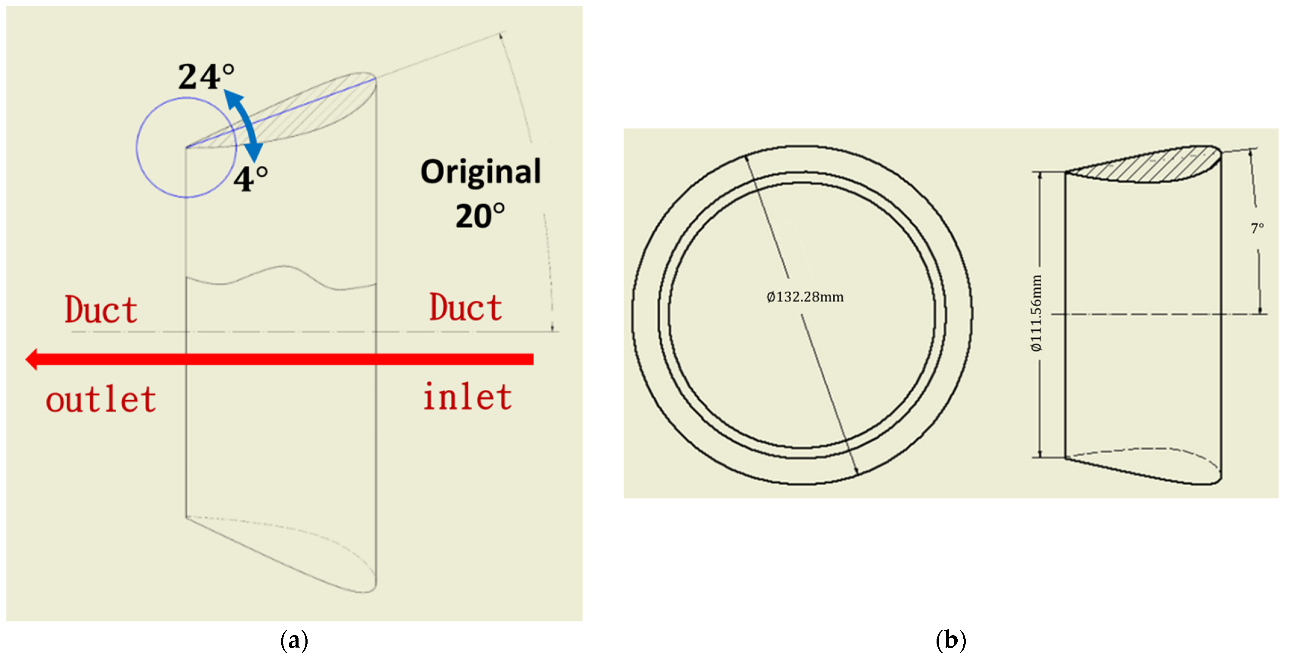
2.1. Geometry
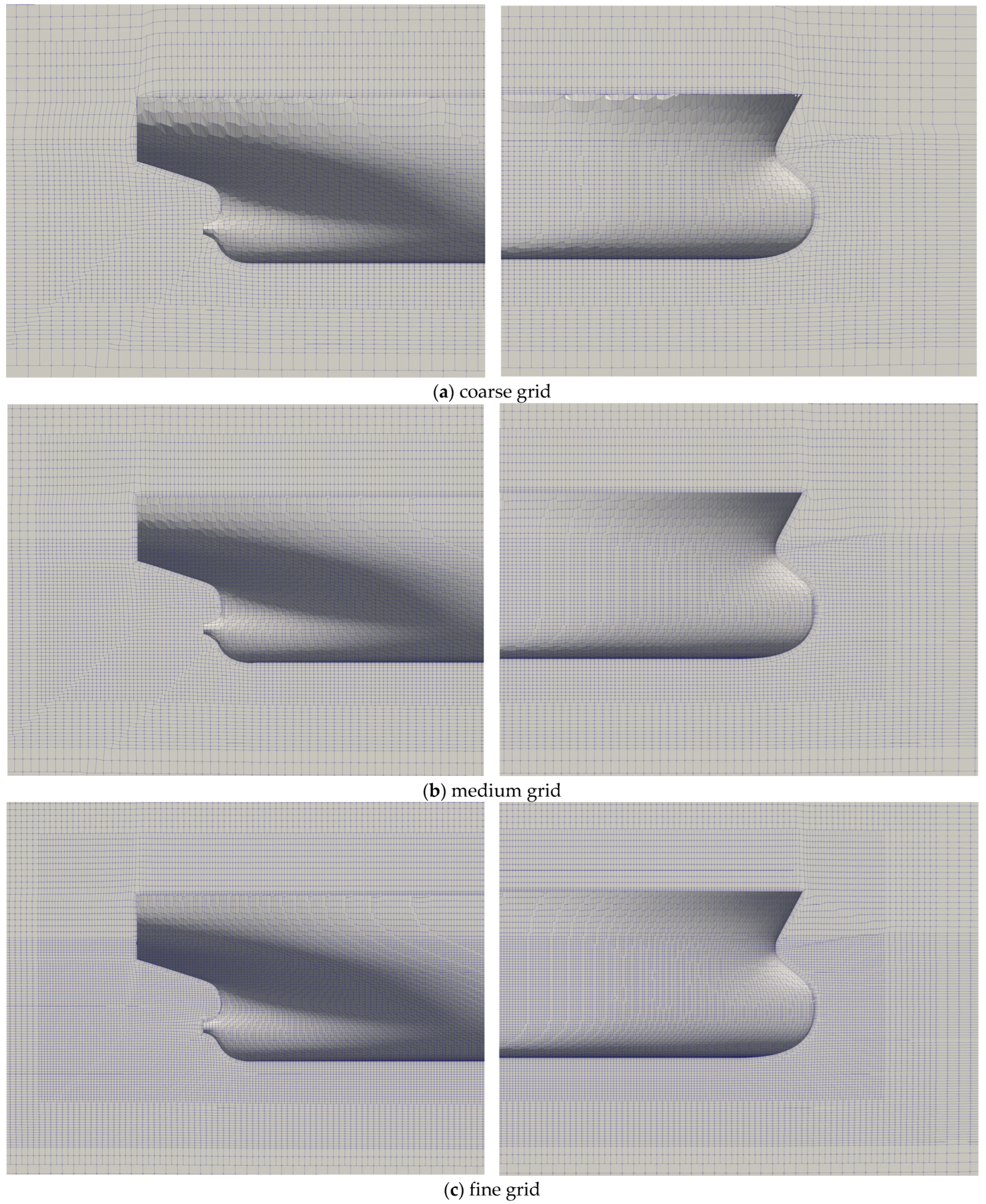
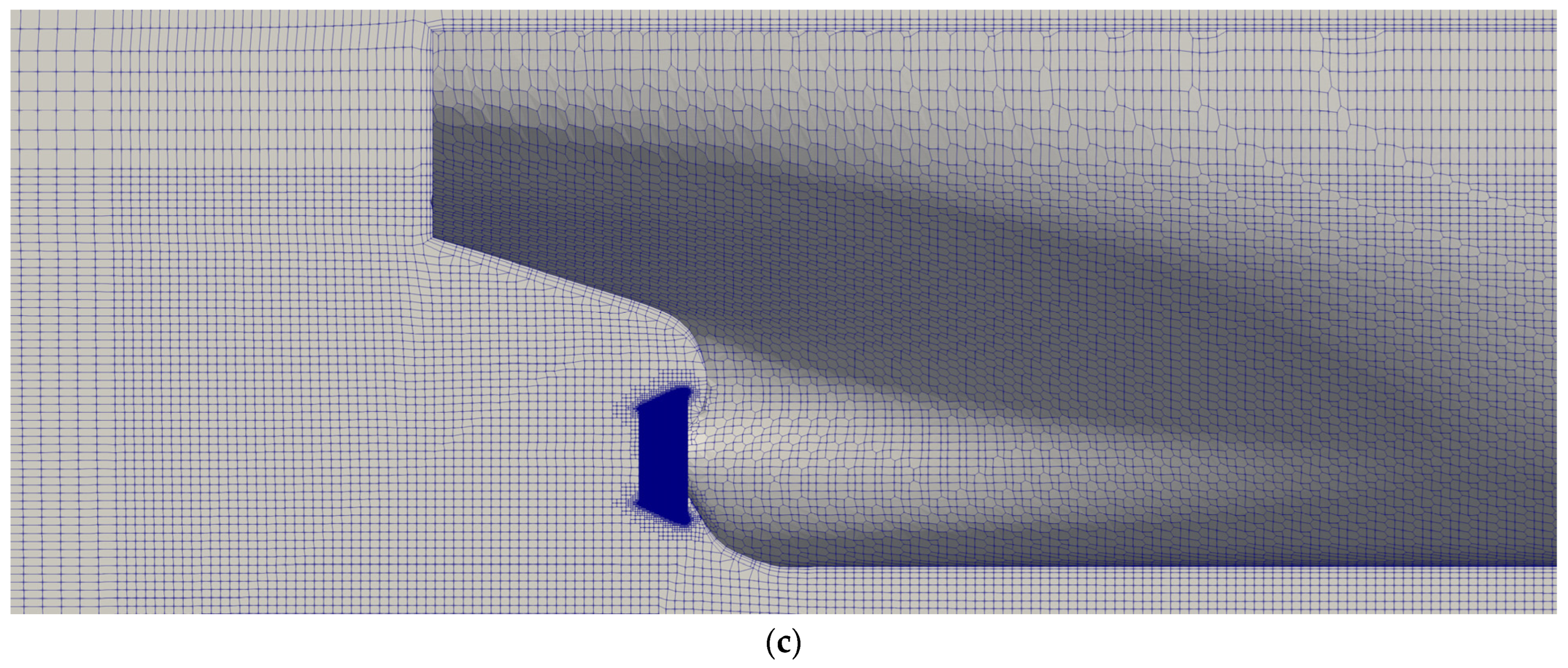
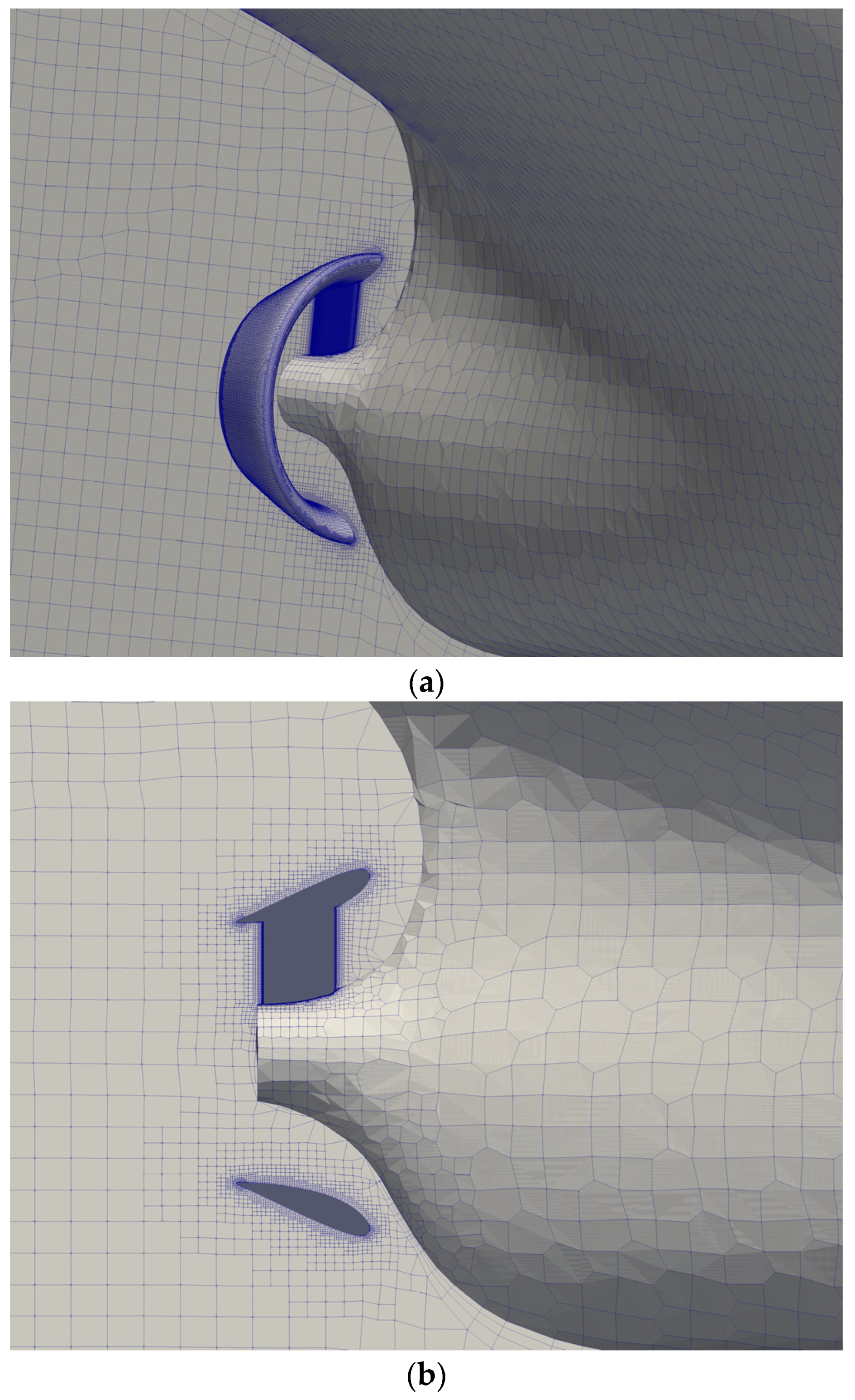
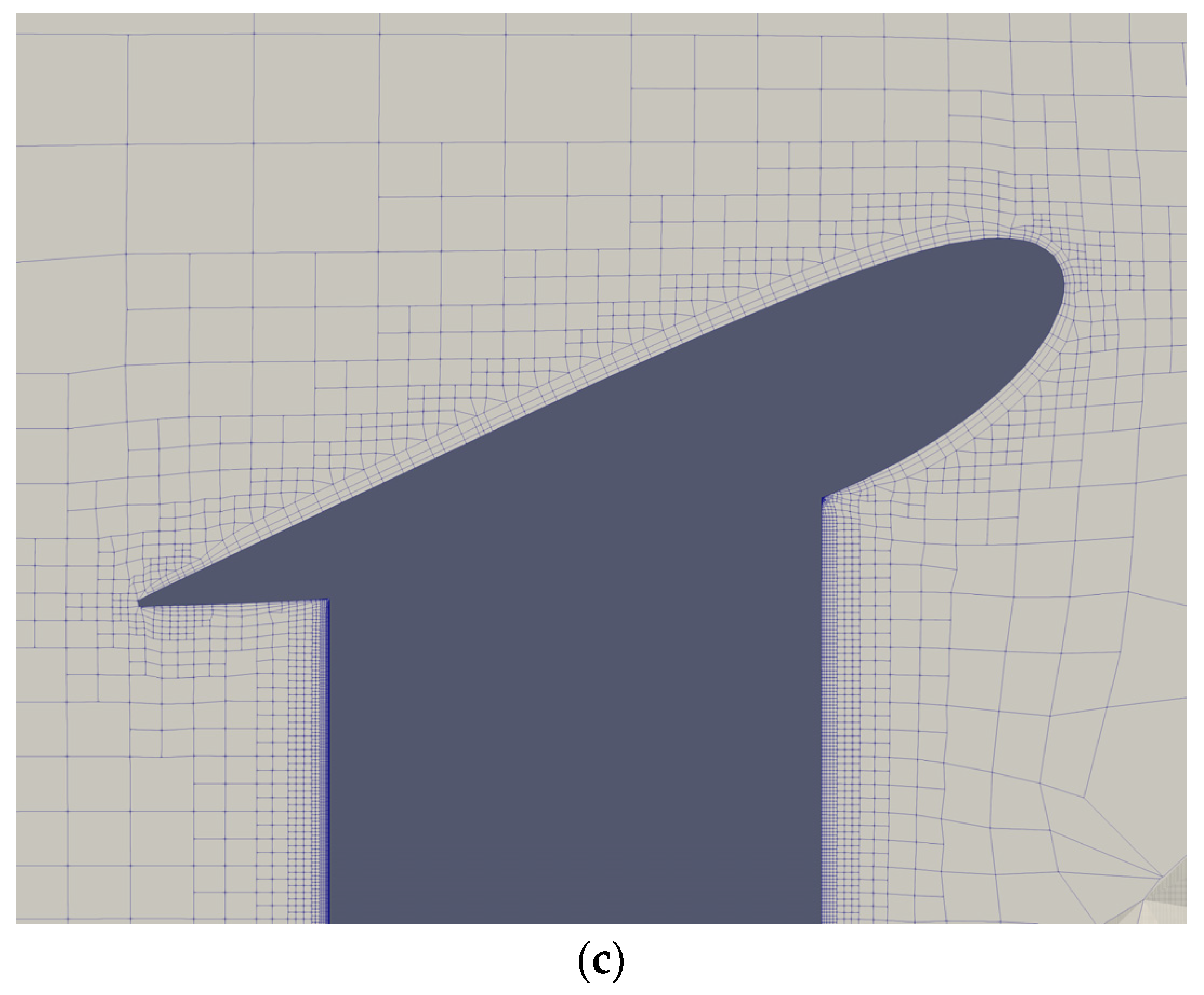
2.2. Grids on the Geometry
2.2.1. Computational domain and JBC hull
2.2.2. JBC Hull with Duct
2.3. Boundary Conditions
2.4. CFD Algorithms
3. Results
3.1. Verification and Validation
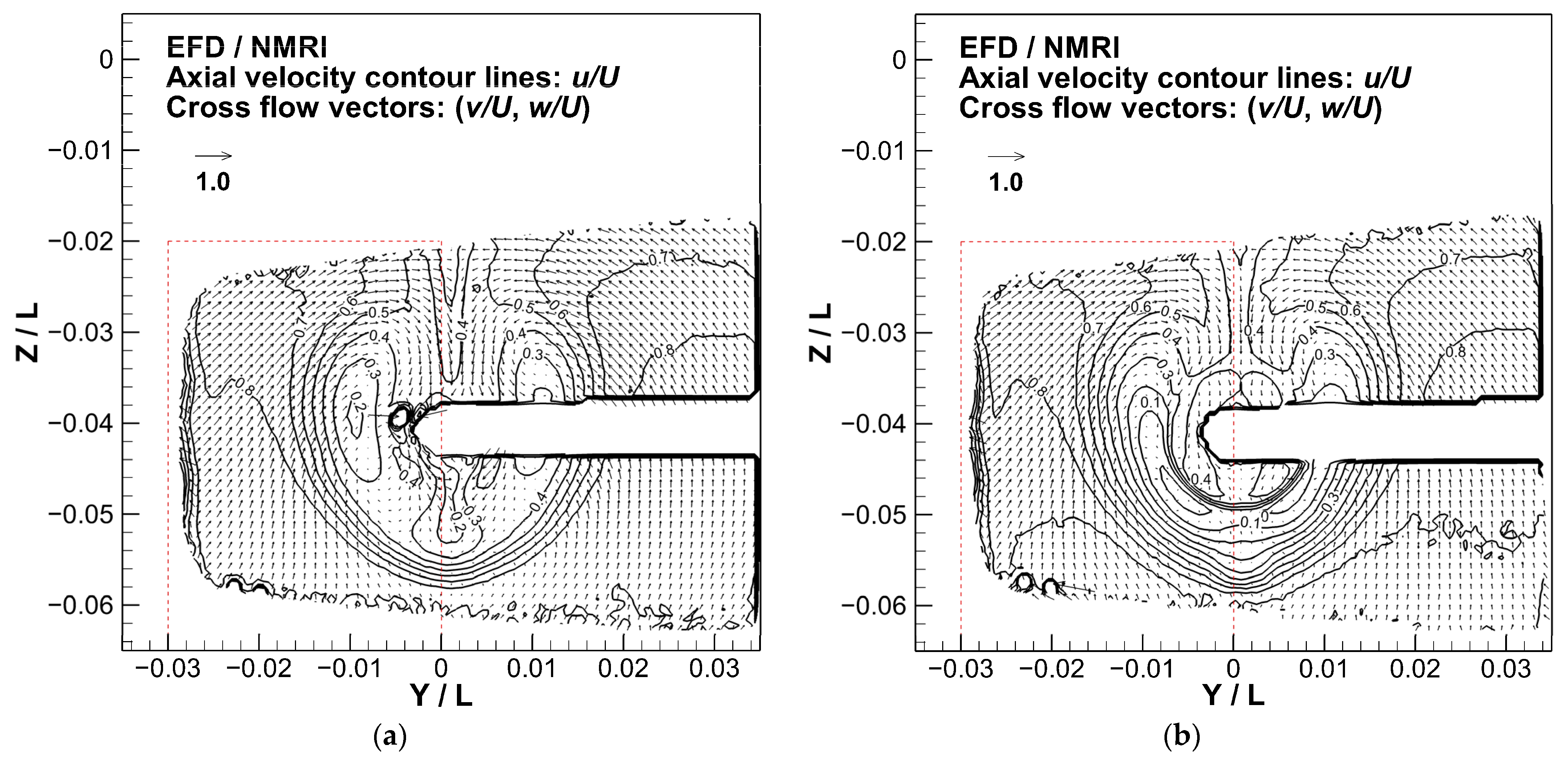
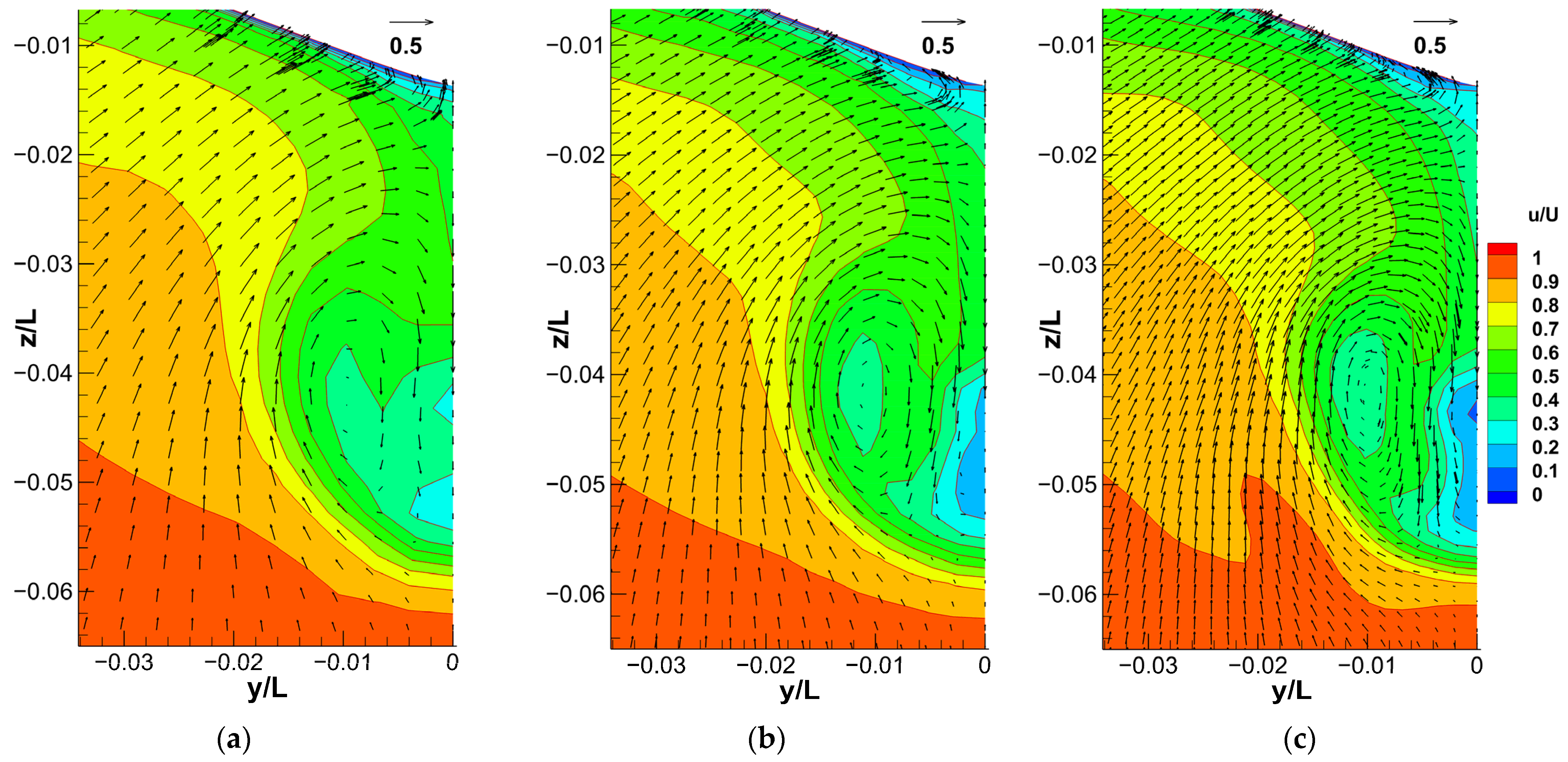
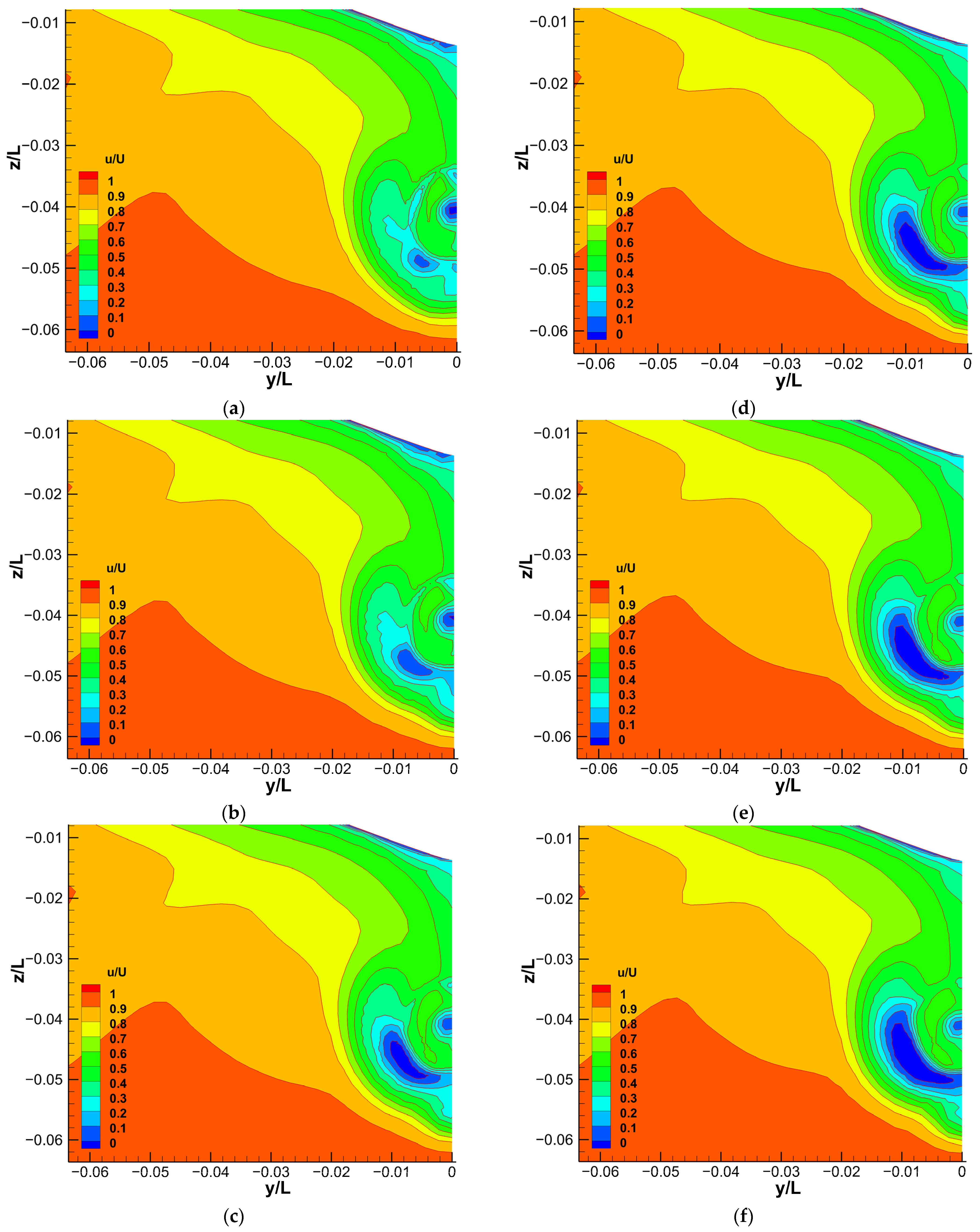
3.2. Nominal Wake Comparison for the Hull without/with the Original Duct
3.3. Duct Design
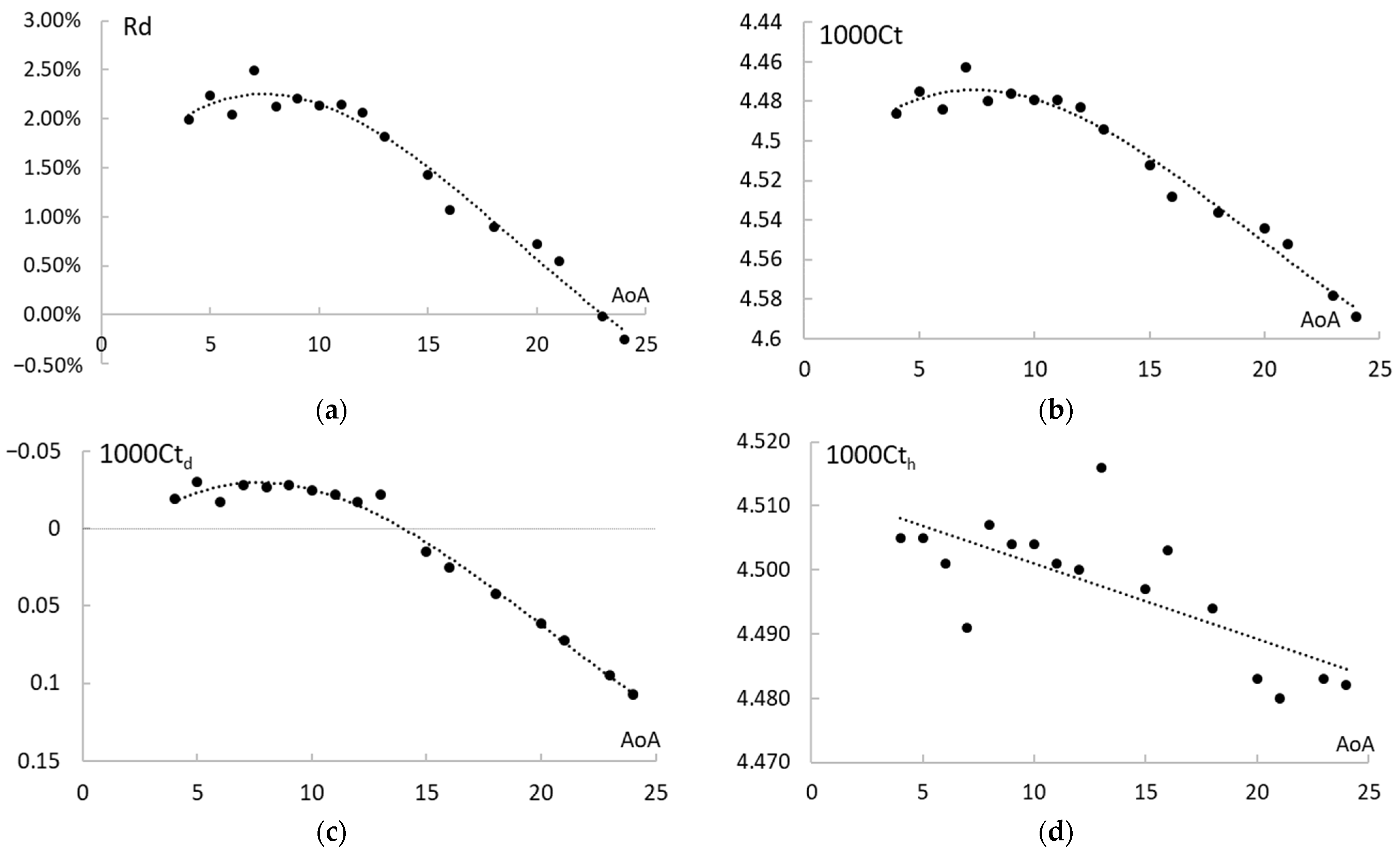
3.3.1. Energy Saving Result
3.3.2. Nominal Wake Analysis
4. Conclusions
Author Contributions
Funding
Institutional Review Board Statement
Informed Consent Statement
Data Availability Statement
Conflicts of Interest
References
- Truong, T.Q.; Wu, P.C.; Aoyagi, K.; Koike, K.; Akiyama, Y.; Toda, Y. The EFD and CFD study of rudder-bulb-fin system in ship and propeller wake field of KVLCC2 tanker in calm water. In Proceedings of the 27th International Ocean and Polar Engineering Conference (ISOPE 2017), San Francisco, CA, USA, 25–30 June 2017. [Google Scholar]
- Truong, T.Q.; Wu, P.C.; Kishi, J.; Toda, Y. Improvement of rudder-bulb-fin system in ship and propeller wake field of KVLCC2 tanker in calm water. In Proceedings of the 28th International Ocean and Polar Engineering Conference (ISOPE 2018), Sapporo, Japan, 10–15 June 2018. [Google Scholar]
- Hino, T.; Stern, F.; Larsson, L.; Visonneau, M.; Hirata, N.; Kim, J. Numerical Ship Hydrodynamics: An Assessment of the Tokyo 2015 Workshop; Springer: Dordrecht, The Netherlands, 2020; pp. 30–31. [Google Scholar]
- Maasch, M.; Mizzi, K.; Atlar, M.; Fitzsimmons, P.; Turan, O. A generic wake analysis tool and its application to the Japan Bulk Carrier test case. Ocean. Eng. 2019, 171, 575–589. [Google Scholar] [CrossRef]
- Yokota, S.; Tokgoz, E.; Wu, P.-C.; Toda, Y. CFD Computation around Energy-Saving Device of Japan Bulk Carrier on Overset Grid. In Proceedings of the Japan Society of Naval Architects and Ocean Engineers, Tokyo, Japan, 16–17 November 2015. [Google Scholar]
- Furcas, F.; Vernengo, G.; Villa, D.; Gaggero, S. Design of Wake Equalizing Ducts using RANSE-based SBDO. Appl. Ocean. Res. 2020, 97, 102087. [Google Scholar] [CrossRef]
- Çelik, F. A numerical study for effectiveness of a wake equalizing duct. Ocean. Eng. 2007, 34, 2138–2145. [Google Scholar] [CrossRef]
- Guiard, T.; Leonard, S. The Becker Mewis Duct®-Challenges in Full-Scale Design and new Developments for Fast Ships. In Proceedings of the 3rd international symposium on marine propulsors, Launceston, Tasmania, Australia, 5–7 May 2013. [Google Scholar]
- Bertram, V. Fuel-Saving Options. In Practical Ship Hydrodynamics, 2nd ed.; Butterworth-Heinemann: Oxford, UK, 2000; pp. 135–141. [Google Scholar]
- Chang, X.; Sun, S.; Zhi, Y.; Yuan, Y. Investigation of the effects of a fan-shaped Mewis duct before a propeller on propulsion performance. J. Mar. Sci. Technol. 2019, 24, 46–59. [Google Scholar] [CrossRef]
- Tokyo 2015 Workshop on CFD in Ship Hydrodynamics. Available online: https://t2015.nmri.go.jp/index.html (accessed on 4 December 2015).
- ITTC 7.5-03-02-03. Available online: https://ittc.info/media/1357/75-03-02-03.pdf (accessed on 3 September 2011).
- ITTC 7.5-03-01-01. Available online: https://ittc.info/media/4184/75-03-01-01.pdf (accessed on 20 September 2008).
- Hirt, C.W.; Nichols, B.D. Volume of Fluid Method for the Dynamics of Free Boundaries. J. Comput. Phys. 1981, 39, 201–225. [Google Scholar] [CrossRef]
- Menter, F.R.; Kuntz, M.; Langtry, R. Ten years of industrial experience with the SST turbulence model, In Proceedings of the 4th International Symposium on Turbulence, Heat and Mass Transfer, Antalya, Turkey, 12–17 October 2003.
- Holzmann, T. The numerical algorithms: SIMPLE, PISO and PIMPLE. In Mathematics, Numerics, Derivations and OpenFOAM®; Holzmann CFD: Loeben, Germany, 2006; pp. 93–121. [Google Scholar]


| Grid Number on Boundaries * | Initial Grid Number (BlockMesh Result) | Final Grid Number (Snappyhex Result) | Layers (Coverage) | y+ | ||||
|---|---|---|---|---|---|---|---|---|
| Nx | Ny | Nz | ||||||
| No duct | Coarse | 30 | 13 | 122 | 47,580 | 590,884 | 3 (94.5%) | 87.3 |
| Medium | 42 | 19 | 168 | 134,064 | 1,571,444 | 3 (99.7%) | 56.6 | |
| Fine | 60 | 27 | 239 | 387,180 | 4,537,454 | 3 (99.2%) | 37.9 | |
| With duct | Coarse | 30 | 13 | 122 | 47,580 | 707,575 | 3 (93.4%) | 84.5 |
| Medium | 42 | 19 | 168 | 134,064 | 2,118,382 | 3 (94.9%) | 52.4 | |
| Fine | 60 | 27 | 239 | 387,180 | 6,186,049 | 3 (98.4%) | 37.4 | |
| 1000Ct | S1 | S2 | S3 | RG | Verified or Not |
|---|---|---|---|---|---|
| Without duct | 4.400 | 4.577 | 5.961 | 0.128 | Yes |
| With duct | 4.393 | 4.544 | 5.886 | 0.113 | Yes |
| E%D | S1 | S2 | S3 | D | UD | Uv%D | Validated or Not |
|---|---|---|---|---|---|---|---|
| Without duct | −2.59% | −6.72% | −38.99% | 4.289 | 1% | 5.26% | Yes |
| With duct | −3.05% | −6.60% | −38.07% | 4.263 | 1% | 4.55% | Yes |
| Rd (%) | 0.16% | 0.72% | 1.27% | 0.6% |
| S1 | S2 | S3 | RG | UD | Uv%S1 | |
|---|---|---|---|---|---|---|
| 1000Ct | 4.310 | 4.463 | 5.836 | 0.111 | 1% | 4.55% |
| Grid number | 6.02 M | 2.20 M | 0.49 M | Verified | (Validated) |
| AoA | 1000Ct | 1000Ctd | 1000Cth | Rd (%) |
|---|---|---|---|---|
| 4° | 4.486 | −0.019 | 4.505 | 1.99% |
| 5° | 4.475 | −0.030 | 4.505 | 2.24% |
| 6° | 4.484 | −0.017 | 4.501 | 2.04% |
| 7° | 4.463 | −0.028 | 4.491 | 2.49% |
| 8° | 4.480 | −0.027 | 4.507 | 2.12% |
| 9° | 4.476 | −0.028 | 4.504 | 2.21% |
| 10° | 4.479 | −0.025 | 4.504 | 2.14% |
| 11° | 4.479 | −0.022 | 4.501 | 2.15% |
| 12° | 4.483 | −0.017 | 4.500 | 2.06% |
| 13° | 4.494 | −0.022 | 4.516 | 1.82% |
| 15° | 4.512 | 0.015 | 4.497 | 1.43% |
| 16° | 4.528 | 0.025 | 4.503 | 1.07% |
| 18° | 4.536 | 0.042 | 4.494 | 0.90% |
| 20° | 4.544 | 0.061 | 4.483 | 0.72% |
| 21° | 4.552 | 0.072 | 4.480 | 0.55% |
| 23° | 4.578 | 0.095 | 4.483 | −0.02% |
| 24° | 4.589 | 0.107 | 4.482 | −0.25% |
Publisher’s Note: MDPI stays neutral with regard to jurisdictional claims in published maps and institutional affiliations. |
© 2022 by the authors. Licensee MDPI, Basel, Switzerland. This article is an open access article distributed under the terms and conditions of the Creative Commons Attribution (CC BY) license (https://creativecommons.org/licenses/by/4.0/).
Share and Cite
Wu, P.-C.; Chang, C.-W.; Huang, Y.-C. Design of Energy-Saving Duct for JBC to Reduce Ship Resistance by CFD Method. Energies 2022, 15, 6484. https://doi.org/10.3390/en15176484
Wu P-C, Chang C-W, Huang Y-C. Design of Energy-Saving Duct for JBC to Reduce Ship Resistance by CFD Method. Energies. 2022; 15(17):6484. https://doi.org/10.3390/en15176484
Chicago/Turabian StyleWu, Ping-Chen, Chin-Wei Chang, and Yu-Chi Huang. 2022. "Design of Energy-Saving Duct for JBC to Reduce Ship Resistance by CFD Method" Energies 15, no. 17: 6484. https://doi.org/10.3390/en15176484
APA StyleWu, P.-C., Chang, C.-W., & Huang, Y.-C. (2022). Design of Energy-Saving Duct for JBC to Reduce Ship Resistance by CFD Method. Energies, 15(17), 6484. https://doi.org/10.3390/en15176484