3.1. Verification and Validation
Table 2 shows the verification result for the ship resistance of JBC hull without/with the original duct. In the Table,
S1,
S2 and
S3 present the total ship resistance coefficient 1000
Ct for the fine, medium, and coarse grid, respectively.
Ct is calculated as follows
where
Rt is the force value (
N) of resistance and
is the water density (998.2 kg/m
3). The wetted surface area
S = 12.2225625 m
2 for JBC bare hull.
S = 12.2711875 m
2 is for JBC with duct including the original duct. It is also used later in
Section 3.3.1 for different duct design, since the area difference among ducts is small compared to the hull.
To check the grid convergence, a ratio
RG is referred as below:
Once
RG is less than 1, it means the resistance difference between the medium and fine grid is smaller than the difference between medium and coarse grid. The so-called monotonic convergence is achieved: as the grid number increases, the resistance difference decreases between two grid densities. Therefore, our CFD method is verified as shown in
Table 2, and the grid independence is confirmed.
For validation, the grid uncertainty
UG is estimated by the suggestion of ITTC 7.5-03-01-01 guideline [
13] and listed in
Table 3. Additionally,
UG is compared against the error
E%D calculated by the following equation
wherein
D is the experimental resistance value provided by T2015 [
11]. If |
UG| is greater than |
E%D| of
S1, the validation is satisfied, i.e., the uncertainty level between CFD and experimental value is below CFD itself.
Table 3 shows that our CFD method is also validated.
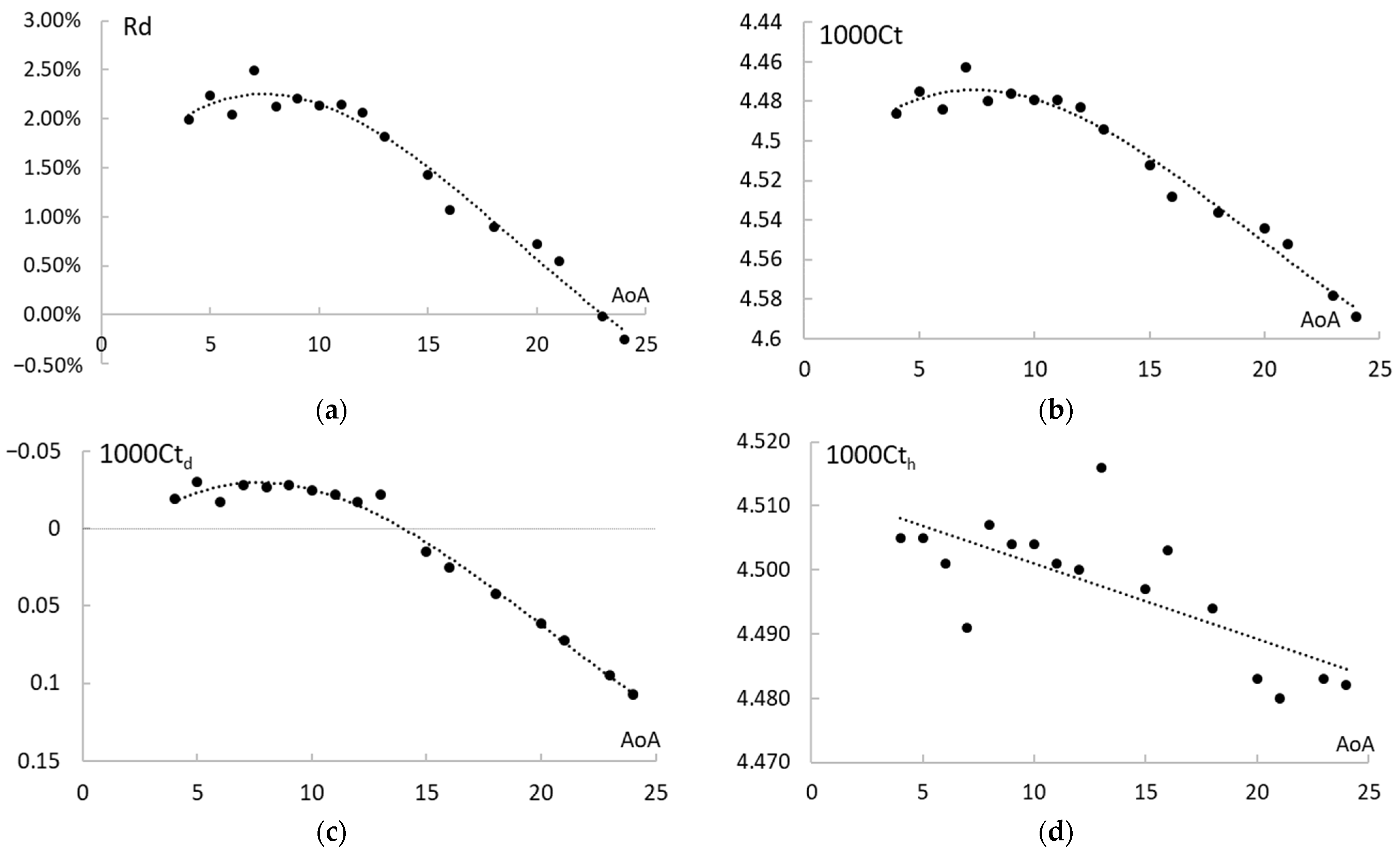
All CFD resistance results over-predict. The error will reduce to around 3% as grid number increases. The energy saving effect of the duct, i.e., ESD, can be evaluated by the resistance reduction
Rd, which is calculated by Equation (4) below:
The
Rd result is also shown in
Table 3. The medium and fine grid can capture the energy-saving effect better than the coarse grid can.
Rd of
S1,
S2 and
D is less than 1%, but for
S2 Rd is larger than 1%. In consideration of computational time consumption and flow field resolution,
S2 grid, i.e., medium grid with grid number 2.1 M with duct, is selected for the duct design. Furthermore,
S2 error is over-predicted at around 7%, which is acceptably small, and its
Rd is 0.72%, which is much closer to experimental 0.6% than
S1 value (0.16%).
The coarse, medium and fine grid are appended with the optimal 7
duct (the detailed result is in
Section 3.3.1) to conduct the grid dependence test. However, the experimental data is not available. The
UD is assumed to be 1%, and the uncertainty is compared with the fine grid result
S1. i.e.,
Uv%S1. As shown in
Table 4, the grid dependence is confirmed by
RG < 1, which means it is verified. The
Uv = 4.55%
S1 with the 7
duct coincides with
Uv = 4.55%
D with the original duct (
Table 3). We assume that the
S1 for the 7
duct can provide the similar error level as the
S1 of the original duct does (3.05%). Therefore, the validation can be considered as satisfied.
3.2. Nominal Wake Comparison for the Hull without/with the Original Duct
In the present work, the propeller is not considered, and only bare hull condition is investigated with and without the duct. The nominal wake analysis studies the velocity field on the propeller plane without a propeller. Although there is no propeller effect here, it still helps to understand how the complicated flow field phenomena of ship wake will influence propeller inflow. Once the propeller is put back in place, those phenomena are no longer observable as the flow field is physically blocked and is occupied by the rotating propeller itself. On the other hand, those phenomena will also be affected by propeller effect, which mainly is propeller suction, i.e., propeller induced velocity.
To have the comparison reference, some related values from the T2015 [
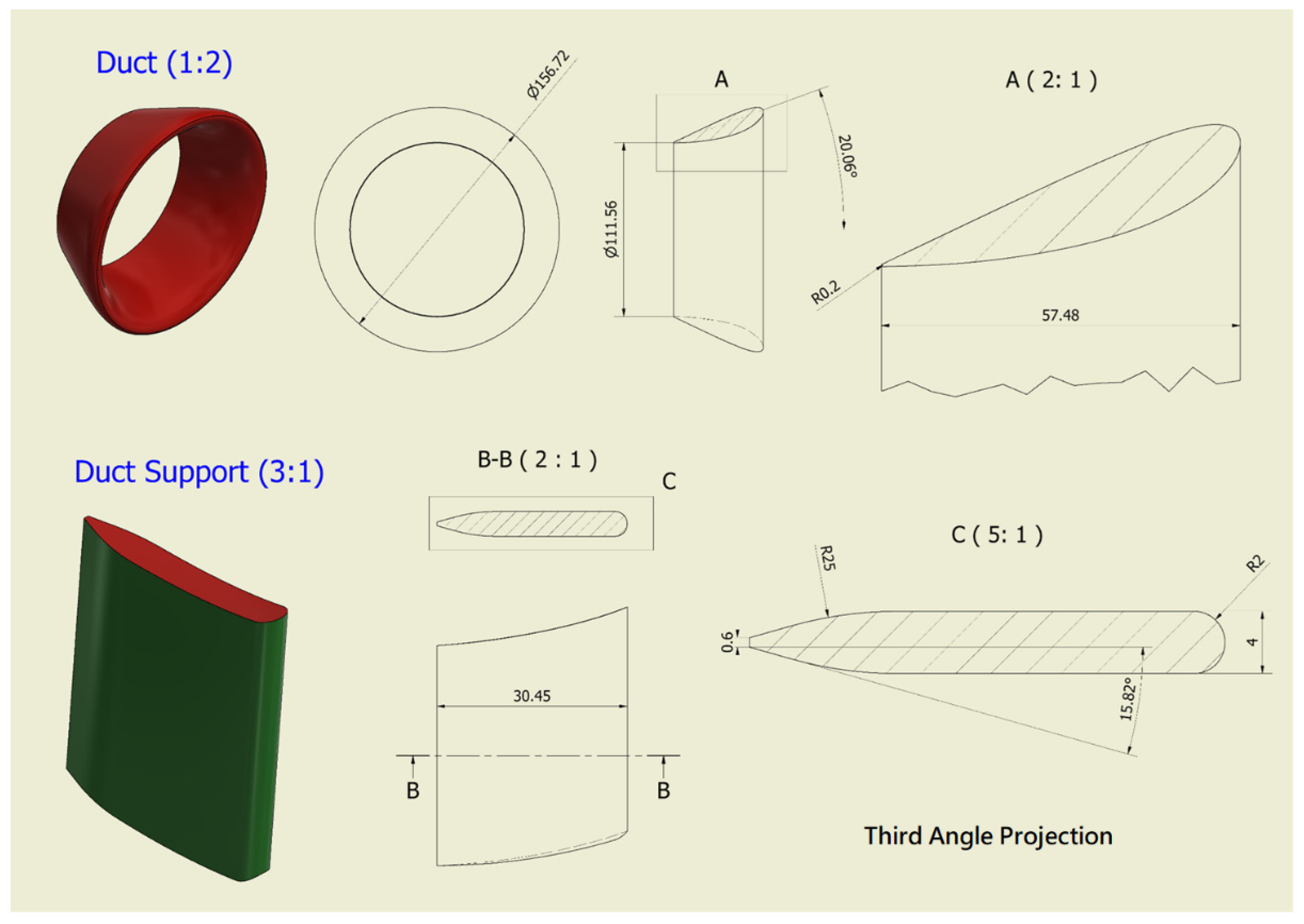
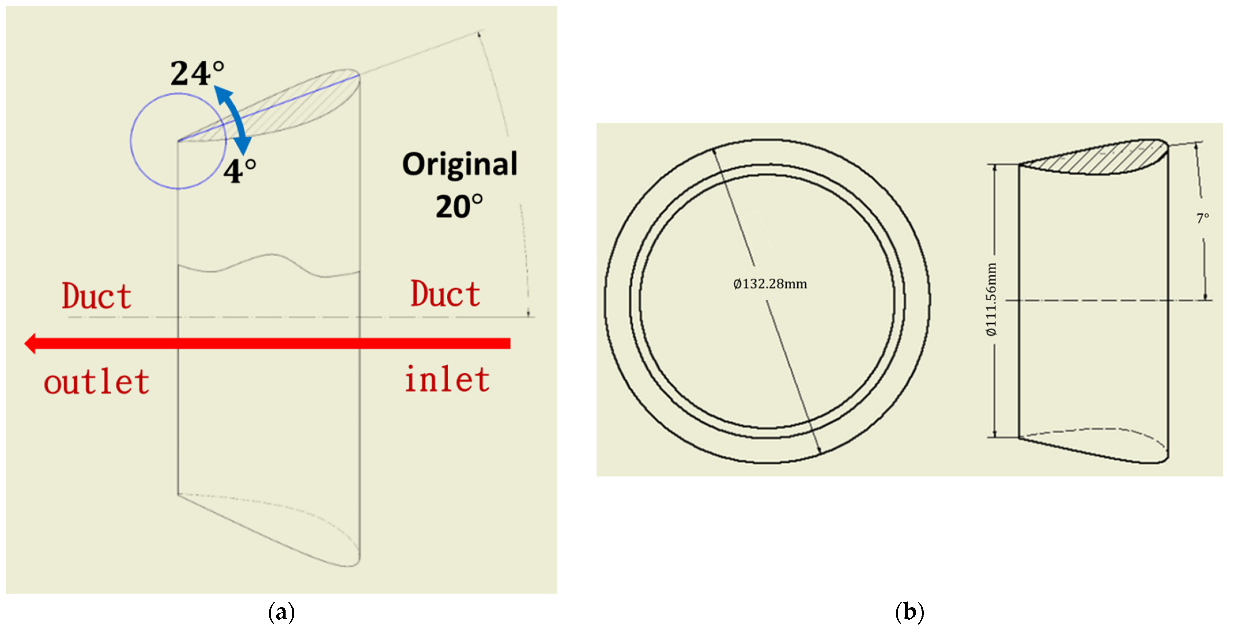
14] release are listed, and are calculated into non-dimensional results as follows. The radius of the duct outlet is 156.72 mm/7000 mm/2 = 0.0112. The radius of the duct inlet is 111.56 mm/7000 mm/2 = 0.00797. Propeller radius
RP/L = 0.203/2/7 = 0.0145. The propeller center is below the water line at
z/L = −0.0404214 and
y/L = 0. Propeller plane in longitudinal direction is at
x/L = 0.985714; thus, the nominal wake is analyzed on
x/L = 0.985714 in our study. The 3-dimensional flow velocity includes
u/U for axial direction,
v/U for side direction, and
w/U for vertical direction. For
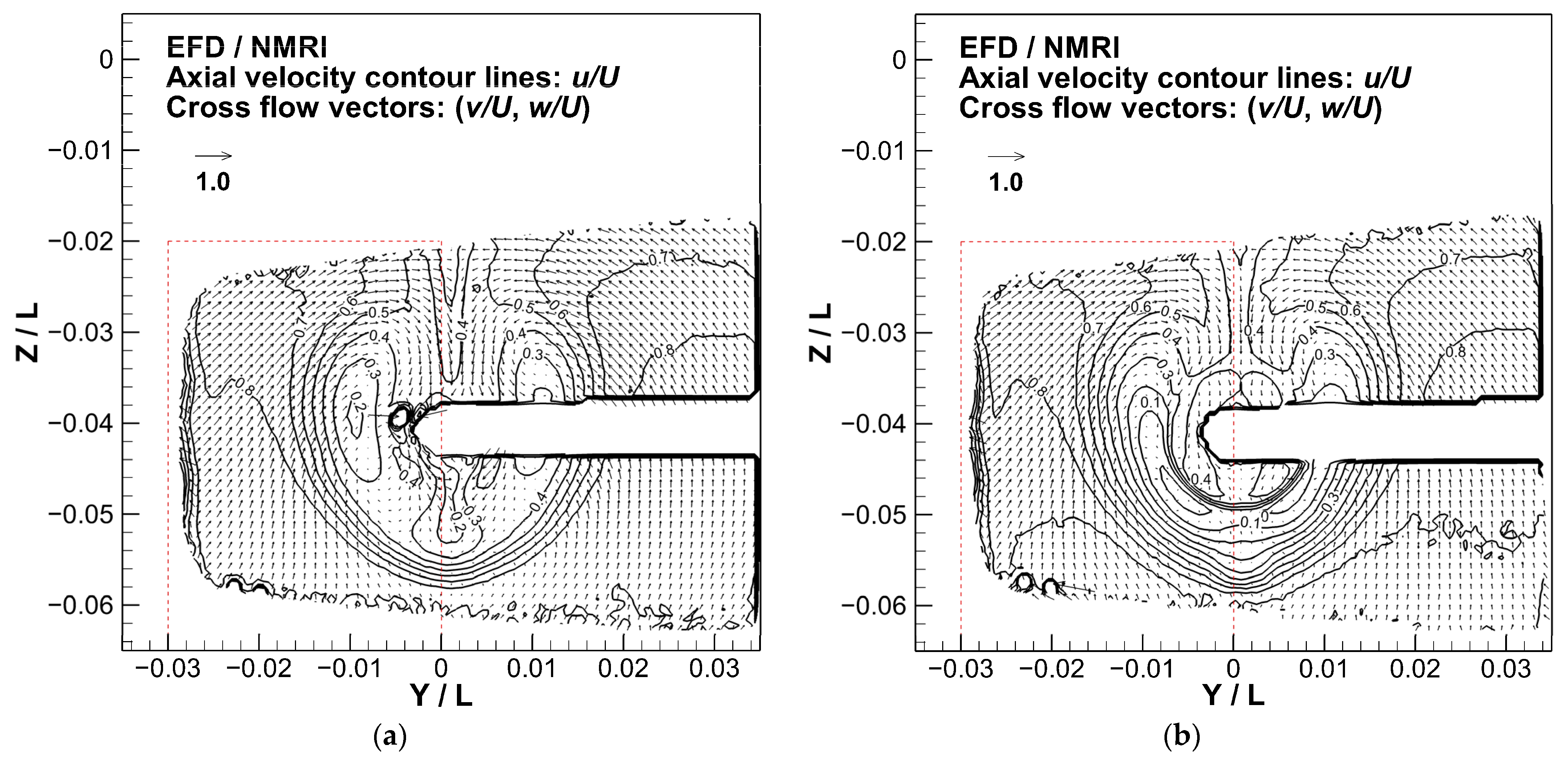
u/U distribution, i.e., nominal wake factor (1 –
wn) distribution, the contour lines are plotted in
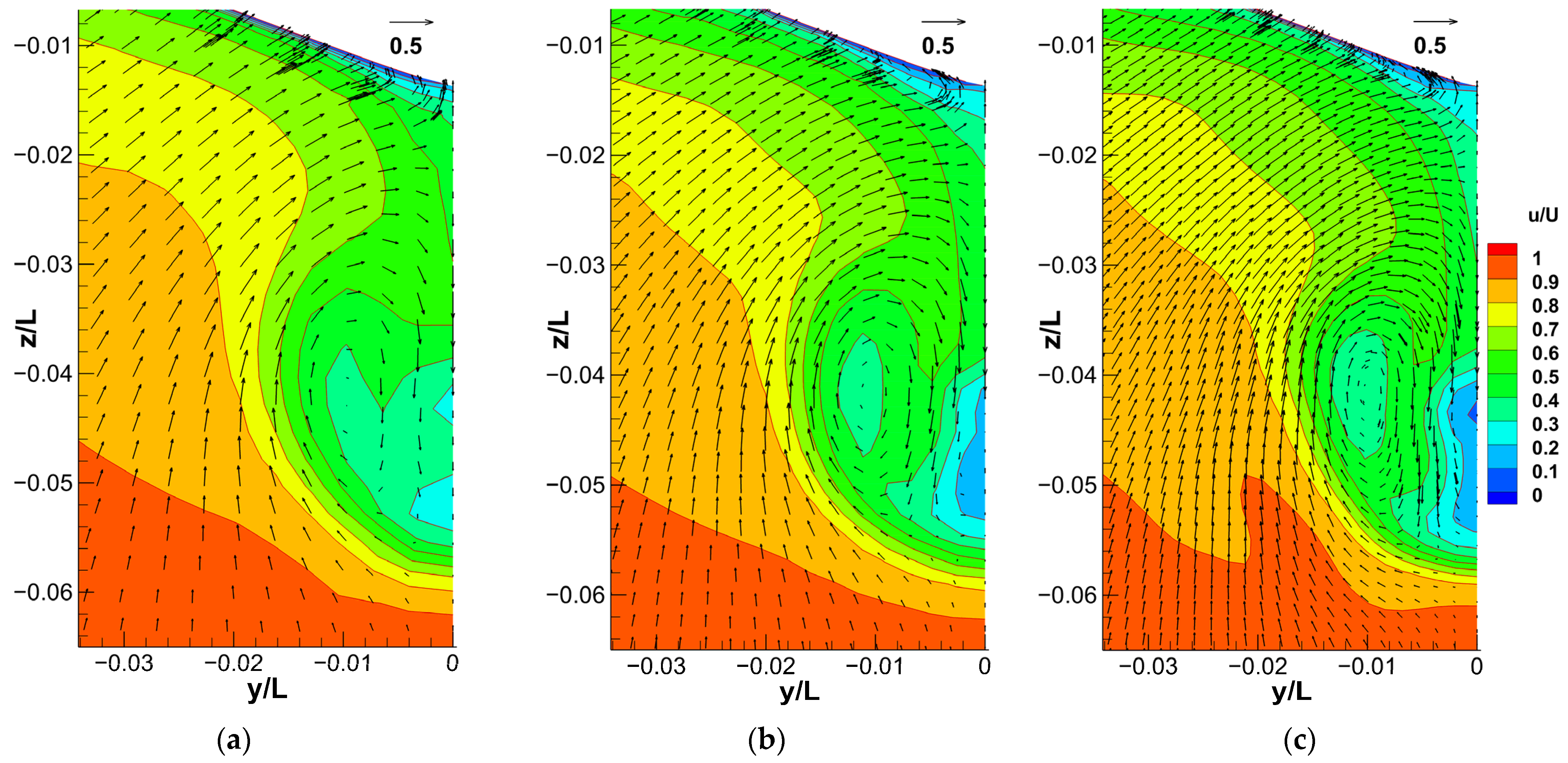
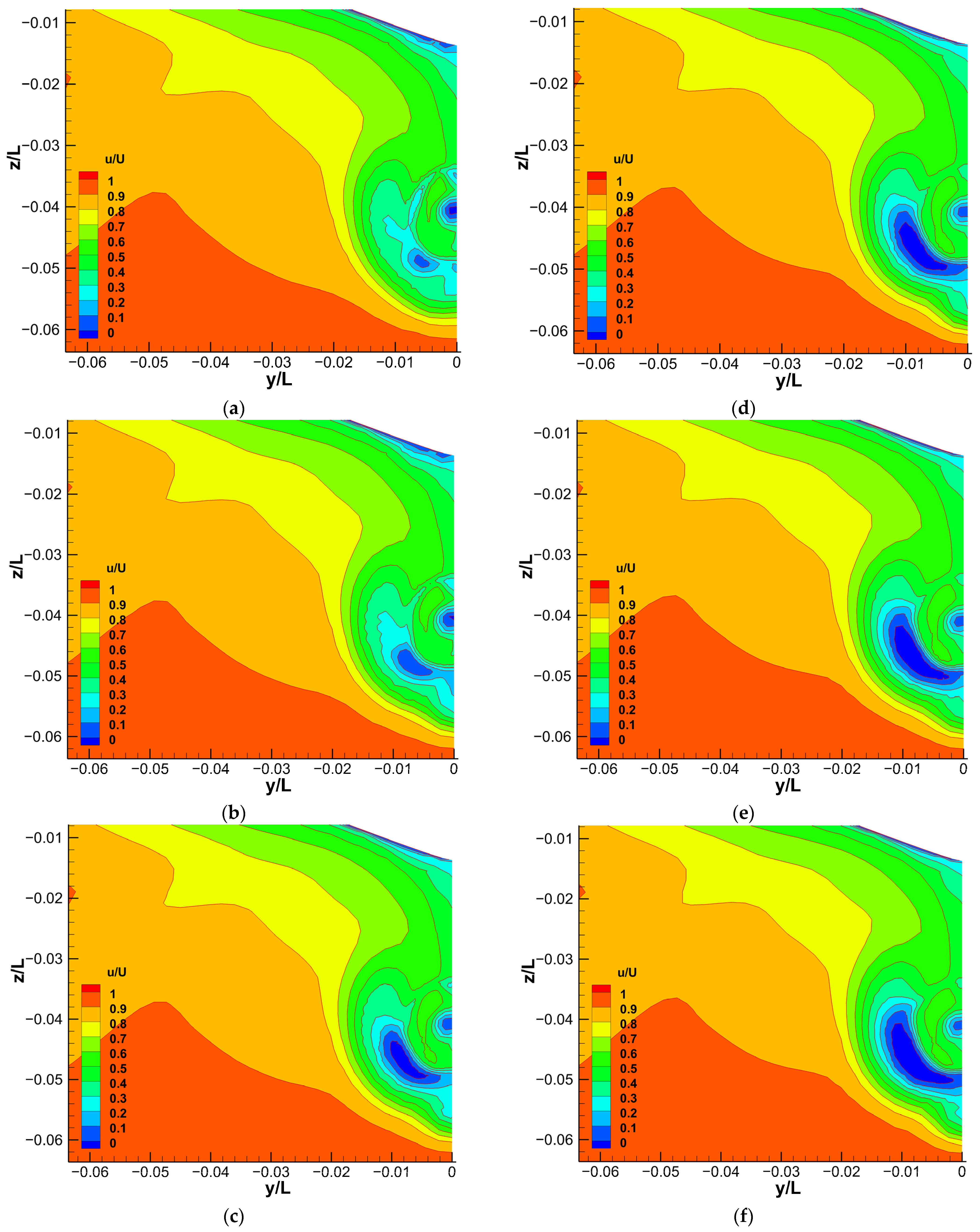
Figure 9 for the experimental measurement without and with duct. The flooded contours of
u/U are drawn for CFD result without the duct in
Figure 10 and with the duct in
Figure 11. In both figures, the coarse, medium, and fine grid results which pass the V&V analysis in
Section 3.1 (
Table 2 and
Table 3) are listed side by side, sharing the same contour legend. In those three figures, the vector fields of (
v/U, w/U) are topped with
u/U for observing vortex behavior.
In the comparison of
Figure 9a and
Figure 10, the flow field phenomena without the duct are well resolved by CFD results such as the bilge vortex beside the propeller center, low-speed area below the propeller center, and upward flow in the far field. All CFD and experiments show the agreement for the location of bilge vortex to be located between
z/L = −0.05 and −0.03 vertically, i.e., almost right next to the propeller center, and around
y/L = −0.01 horizontally. The bilge vortex is accompanied by the region of
u/U = 0.3–0.5. The contour line of
u/U = 0.4 forming a U-shaped pattern surrounds the propeller center on the propeller plane. From the coarse to fine grid, the U-shaped patterns become smoother with a clearer bilge vortex. However, in the experiment, near the core of the bilge vortex
u/U reaches 0.2, which cannot be preserved by CFD. It may require a much finer grid to capture the
u/U = 0.2 core. The secondary vortex is induced by the bilge vortex inside the low-speed area
u/U < 0.3. As the grid densities increase, the pattern of the low-speed area with clearer secondary vortex will also get closer to the experimental pattern. Inside the low-speed area, the medium and fine grid result are both capable of capturing the
u/U = 0.2 contour line, and the contour pattern of the fine grid result agrees with the experimental result better. In the far field, the upward flow with the vector component points toward
y = 0, due to the ship stern geometry and bilge vortex rotation.
Obviously, the nominal wake would be influenced by the appearance of the original duct comparing
Figure 9a to
Figure 9b for the experiment, and
Figure 10 to
Figure 11 for the simulation. In
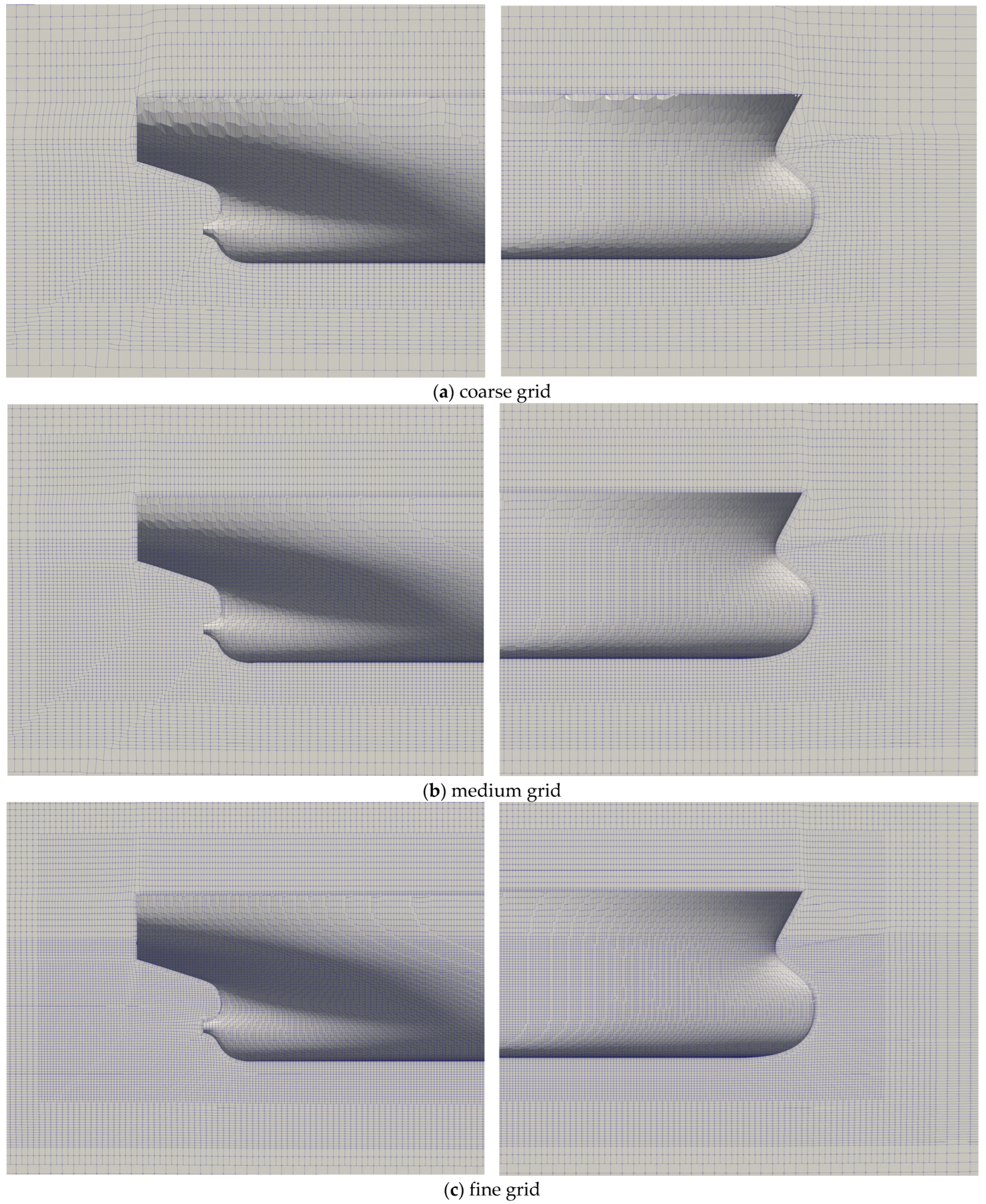
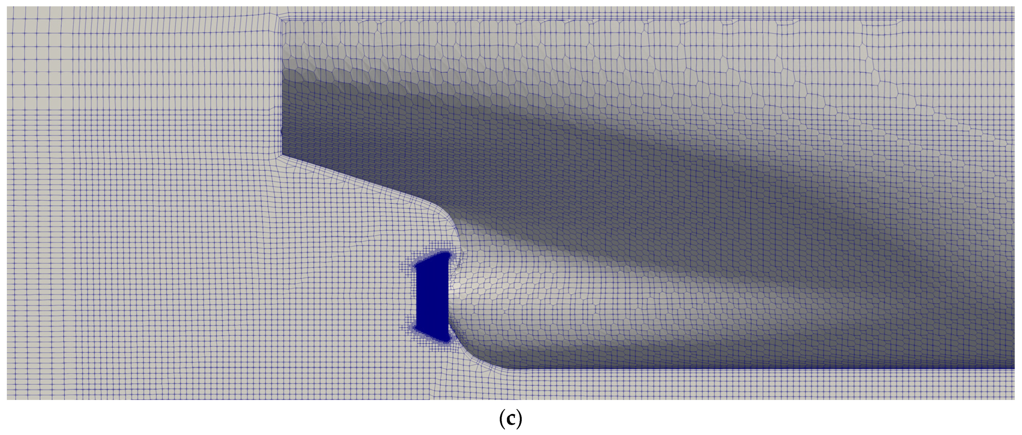
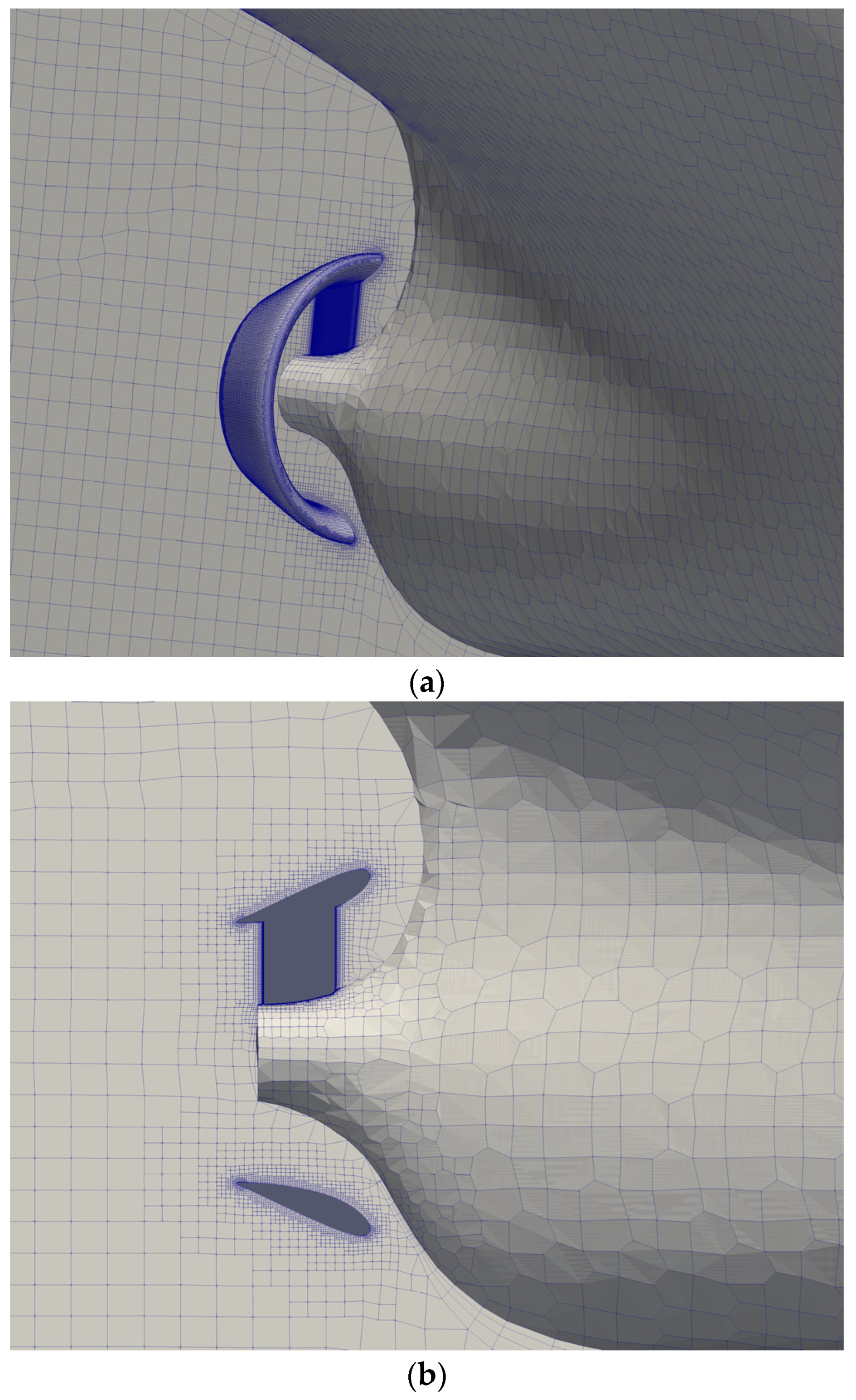
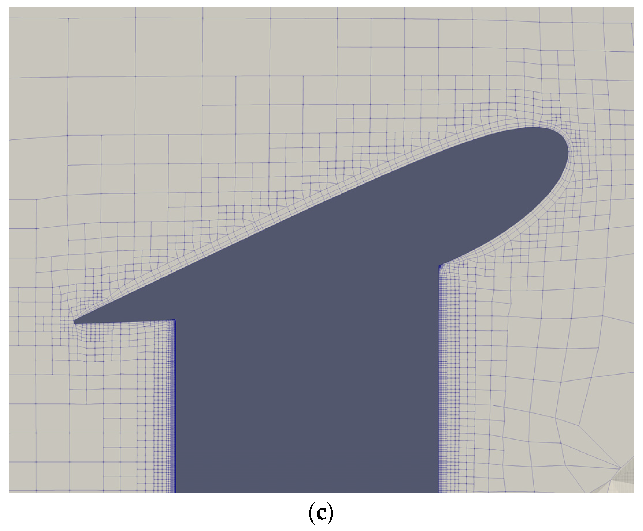
Figure 11, the simulation vector fields are interpolated to 2D uniform spacing grids, which are the same grid used for coarse, medium, and fine grids. This is because the grid is relatively dense around the duct (see
Figure 6 and
Figure 7) compared with the other part of the flow field. The original vector field will block the view on the propeller plane even in the coarse grid. With the duct effect, the bilge vortex becomes smaller and moves upward to
z/L = −0.04~−0.03, but its horizontal location is still around
y/L = −0.01 horizontally. The low-speed area below the propeller center disappears and the flow velocity is accelerated evenly to
u/U = 0.5–0.6. However, a severe flow separation occurs behind the lower part of the duct, which implies that the duct can be further improved. The CFD captures the above-mentioned flow field characteristics that the experiment measures. The main deviation of CFD is the area of reverse flow inside the flow separation, i.e.,
u/U < 0 or negative flow velocity, is larger than experimental result. It also explains that the CFD resistance is over-predicted in
Table 2. The fine grid predicts a closer flow separation profile showing one isolated area for
u/U < 0 and the continuous contour lines for
u/U > 0. For the medium grid result, the contour lines of
u/U < 0 and
u/U = 0.1 are isolated. For the coarse grid result, contour lines of
u/U < 0 and
u/U = 0.1 are two isolated areas. Unlike the coarse grid, the medium and fine grid can resolve the profile of the experiment-like contour lines of
u/U = 0.5–0.8 below the duct. Those contour lines protrude downward along the center plane with the secondary vortex, which is now outside the propeller radius.
Although the finer grid resolves the flow field and agrees with the experiment in more detail, it may reveal new or numerical phenomena. In
Figure 10c, for the case without the duct, the
u/U = 0.9 contour line of the fine grid result shows a bulge in the far field around
y/L = −0.02 and
z/L = −0.05 inserting into
u/U = 0.8–0.9 area. The similar contour bulge can also be observed for the with-duct result for
u/U = 0.8 and 0.9 in
Figure 11c (fine grid). Without or with the duct, this does not exist in the experiment, coarse and medium grid (see
Figure 9,
Figure 10a,b and
Figure 11a,b). In the experiment results,
y/L = −0.02 and
z/L = −0.05 are around the measurement boundary in the portside. Thus, the contour profile in the starboard side shall be considered.
To understand the mechanism of the energy saving and resistance reduction caused by the duct,
Figure 12 analyzes the velocity difference between the CFD results with and without the duct on the propeller plane, i.e., nominal wake velocity difference. The medium grid results are selected here, since their
Rd is close to the experimental value (
Section 3.1 and
Table 3). Furthermore, the medium grid is selected for the duct design after the V&V analysis.
Table 3 also indicates
S2’s error difference (6.72% − 6.60% = 0.12%) is smaller than
S1’s (3.05% − 2.59% = 0.46%). In addition, the fine grid is not selected here because of the bulge of
u/U contour line in the far field, which doesn’t exist in the experiment as discussed previously. On the other hand, the grids without and with the duct are different. Thus, the
u/U was first interpolated from the without-duct to with-duct grid, and then subtracted from the
u/U with the duct to obtain the velocity difference Δ
u/U:
The most interesting finding in
Figure 12 is the Δ
u/U = 0–0.1 area. The axial flow velocity is accelerated by the duct not only inside the duct (excluding the area behind the propeller shaft), but also in the far field behind the main hull body. This means the majority of the velocity increases less than
0.1U, but covers a very large area especially behind the ship hull. As a dimension reference, see the left end of the horizontal axis of
Figure 12:
y/L = −0.08 is around the portside length of the ship beam (0.5
BWL/
L = 1.125 m/7 m/2 ~ 0.080). This velocity increases up to 0.2–0.4
U in the lower part inside the duct. In the lower position, a band region with 0–0.1
U increase is observed in
y/L = −0.01~0 and
z/L = −0.055~−0.052. Thus, the low-speed area below the propeller center without the duct has been eliminated successfully inside the duct and behind the duct bottom. However, a small area of Δ
u/U = −0.2~0 is found around
z/L = −0.06 near the center plane, implying that the low-speed area remains below the duct bottom. In other words, the low-speed area is not eliminated sufficiently by the duct. A major area of Δ
u/U < 0 as low as −0.4 corresponds to the bilge vortex location and separation flow behind the duct. This is proof that the nominal wake can be further improved by the duct design in the next section.
The small flow separation occurs after the truncation end of the stern tube. Since it is out of measurement range in experiment, it can only be seen in CFD results. With duct (
Figure 12), a clear core is shaped by circular contour lines and low flow speed (
u/U < 0.2) at
z/L = −0.04 and
y/L = 0, i.e., propeller shaft end or propeller center. Without the duct (
Figure 11), the core is less clear, connecting with the top of the low-speed area and located slightly below the propeller center. As the grid density increases, the separation core is clearer and the
u/U with the duct (
Figure 11) is lower than without the duct (
Figure 10). This is evidence that the flow separation deteriorates due to the duct. The accelerating duct causes higher velocity passing the truncation end, and the flow separates more severely with lower
u/U inside. The Δ
u/U < 0 core around
z/L = −0.04 and
y/L = 0 in
Figure 13 also illustrates this flow situation.


