Article

Alternative Simplified Analytical Models for the Electric Field, in Shoreline Pond Electrode Preliminary Design, in the Case of HVDC Transmission Systems

by
George J. Tsekouras
1,2,*,
Vassiliki T. Kontargyri
1,2,
John M. Prousalidis
3,
Fotios D. Kanellos
4,
Constantinos D. Tsirekis
1,5,
Konstantinos Leontaritis
5,
John C. Alexandris
5,
Panagiota M. Deligianni
1,5,
Panagiotis A. Kontaxis
1,2 and
Antonios X. Moronis
1
1
Department of Electrical and Electronics Engineering, University of West Attica, 250 Thivon Str., Egaleo, 12241 Athens, Greece
2
School of Electrical and Computer Engineering, National Technical University of Athens, Iroon Polytechniou 9, Zografou, 15780 Athens, Greece
3
School of Naval Architecture and Marine Engineering, National Technical University of Athens, Iroon Polytechniou 9, Zografou, 15780 Athens, Greece
4
School of Electrical and Computer Engineering, Technical University of Crete, University Campus, Akrotiri, 73100 Chania, Greece
5
Hellenic Independent Power Transmission Operator, Dyrrachiou 89 & Kifissou, Sepolia, 10443 Athens, Greece
*
Author to whom correspondence should be addressed.
Energies 2022, 15(17), 6493; https://doi.org/10.3390/en15176493
Submission received: 15 July 2022 / Revised: 28 August 2022 / Accepted: 30 August 2022 / Published: 5 September 2022
(This article belongs to the Special Issue Power System Dynamics and Renewable Energy Integration)

Abstract

:
In Greece, a new bi-polar high voltage direct current (HVDC) transmission system with a ground return was designed with nominal characteristics of ±500 kV, 1 GW, between Attica in the continental country and the island of Crete, which is an autonomous power system based on thermal diesel units. The interconnection line has a total length of about 380 km. The undersea section is 330 km long. In this paper, the use of the Aegean Sea as an active part of the ground return, based on shoreline pond electrodes, was proposed to avoid EUR 200 Μ of expenses. According to the general guidelines for HVDC electrode design by the International Council on Large Electric Systems (CIGRE) working group B4.61/2017, the electric field and ground potential rise of shoreline electrodes should be studied to analyze safety, electrical interference and corrosion impacts related to the operation of the electrodes. Two kinds of studies are available; one is a simplified approach based on a spherical/pointed electrode centered at the edge of the seashore and seabed, assuming it to be sloping to the horizontal, and the other is a detailed simulated model using a suitable electric field software package. The first approach usually gives more unfavorable results than the second one, especially in the near electric field, while it can not take into account obstacles, i.e., dams, near to electrode position. The second approach demands a detailed description of the wider installation area, which cannot be available during the preliminary study, significant computational time and considerable financial resources for the purchase of a reliable specialized software package. In this research, a two-step modification of the CIGRE simplified model was proposed. The first modification deals with the obstacles in the near electric field, and the second modification deals with the use of a linear current source (instead of a point one), which can give more accurate results. Additionally, the electric field for complex electrode formation is calculated by applying the superposition method, which can be easily achieved using a common software package, i.e., MATLAB. The proposed simplified approaches were applied on shoreline pond electrode locations for the Attica–Crete HVDC interconnection line (between Stachtoroi island in Attica and Korakia beach in Crete), allowing the preliminary study to be conducted swiftly, giving satisfactory results about electric field gradient, ground potential rise and resistance to remote earth of electrodes stations for the near and far electric field.

1. Introduction

The history of high voltage direct current interconnections (HVDC) begins in New York with Th. Edison at about 1880 [1]. This was followed by individual HVDC interconnections [2,3,4]. Currently, their use is widespread in offshore wind parks [5,6,7,8,9]. Many technical guidelines have been written about HVDC interconnections, mainly by the International Council on Large Electric Systems (CIGRE) [10,11,12,13,14,15,16,17,18,19,20,21,22]; the Institute of Electrical and Electronics Engineers (IEEE) [23,24,25,26,27,28,29,30]; the International Electrotechnical Commission (IEC) [30,31,32,33,34,35,36,37,38,39,40,41,42]; Electrical Power Research Institute (EPRI) [43,44,45,46]; Energy Department—Oak Ridge National Laboratory, USA [47,48]; Det Norske Veritas (DNV) [49]; and the European Commission [50]. These technical guidelines solve issues such as the configuration of networks and their general characteristics [10,19,25,34,38,43]; the design of individual components, such as transformers [11,12,15,23,24,30,39,40,41,42], electrodes [17,34,45,46,47], switches [18], insulators [26], cables [27,37] and reactors [29]; the environmental/acoustic/electromagnetic effects [13,31,32,36,44,48]; the feasibility of the relevant interconnection projects [14]; the configuration of special purpose networks, such as wind farms [16,49,50]; control and protection techniques of the entire HVDC network [20,22,28]; and testing [29,33,37].
The Hellenic Independent Power Transmission Operator (IPTO) studied, in 2018–2019, the bi-directional interconnection between the island of Crete and mainland Greece in the region of Attica, where there is a 400 kV AC high voltage network, in order to reduce the operation of petroleum thermal power plants and increase the penetration of renewable energy sources in Crete. The required power of the interconnection is 1 GW with a length of at least 380 km, of which the largest part (330 km) is underwater, as shown in Figure 1 [51]. Therefore, the interconnection took place with HVDC in order to reduce the required reactive power due to the existence of cable capacities (where it is only required by the inverters) and to achieve the stability of the electric power system. An HVDC bipolar heteropolar configuration with a nominal power of 2 × 500 MW, at a nominal voltage of ±500 kV DC and voltage source converters, was selected. The return is made via land, as EUR 200 M is saved. Considering that seawater is a much better conductor than the land (at least 100 times lower resistivity), the ground return beyond the sea was proposed by placing two electrode stations in the sea. Near Attica, the island of Stachtoroi was chosen, where the nearest residential area is located at a distance of about 8 km, so that there is no nuisance to the inhabitants (especially from electrochemical erosions). The distance from the 400 kV High Voltage Substation where the inverters are installed is less than 20 km (Figure 2). Near the island of Crete, the electrode station is constructed on the deserted Korakia beach, which is accompanied by the respective converters in the area of Damasta (Figure 3). In addition, the two specific sites meet various criteria, such as geophysical, geological, hydrological, seismological, volcanic, exclusion zones, licenses, the possibility of construction, etc. In addition, electrochemical corrosion should be eliminated in nearby installations. Step and touch voltages should also be eliminated according to IEC 60749-1:2007 [17] (pp. 59–70). From the six usual types of electrodes (land–shallow horizontal, land vertical, land–deep well, sea, shore–beach, shore–pond) according to [17] (p. 19), the shoreline pond electrode was selected for which the determination of the electric field and the potential rise was calculated according to the guidelines of CIGRE B4.61 675:2017 [17]. Based on [17] (pp. 109–120), two methods can be applied during its preliminary design:
  • Simplified analytical method: Electric current is injected at points, and it is considered that space is divided into a soil hemisphere and the area of air [17] (pp. 118–119), thus solving the problem with a simple application of electric field and potential equations;
  • Computational method: Numerical methods are applied for solving electric field problems in order to calculate ground potential rise, electrode resistance, etc. [17] (pp. 119–120). The input data are the configuration, the electrical resistivity of the conductors in the area, especially the resistivity of the ground, which is determined by geophysical methods, such as electrical resistivity tomography and magnetotelluric tomography [52,53], which are extremely time-consuming and costly.
An analytical method similar to CIGRE B4.61 675:2017 [17] is described in IEC TS 62344:2013 [34] (pp. 30–32), with the difference that the air occupies a hemisphere, the water forms a “wedge” of a specific angle, and the rest is homogeneous soil. It is based on Rusck methodology [54], which determined the electrode resistance, electric field strength and current density in the inland ground and seawater, which was repeated in [55] (pp. 465–476), [56,57,58]. In addition, there is the Uhlmann method [57] and [59] (pp. 267–272), which discusses the issue of sea electrodes at a distance from the shore, but considering the ground and the seabed completely insulated. The detailed solution of the field of a shoreline pond anode electrode is mentioned in technical reports about Italy–Greece Interconnection, such as [60].
EPRI proposes the use of numerical algorithms using resistivity data from geophysical methods [45], which are more widely used in grounding electrodes [61] but also in sea electrodes [58,62,63]. In [62], both near and far electric fields were analyzed, using the numerical methods of hemispheroidal, finite volume element and inclined layer, and finally proposes the use of the first two methods [64,65] that have finite limits on the volume of water for the calculation of the scalar potential and ground potential. In [63,66], the use of the finite element method for near-field analysis was suggested. Alternatively, semi-analytical methods can be used, such as the complex images method with a “generalized pencil of functions” interpolator, achieving numerical convergence and solution stability with satisfactory results in the HVDC electrode study [67], which was confirmed with the help of finite elements in grounding systems [68]. Numerical methods can also be used to draw useful conclusions about the problems that stray currents of marine electrodes can cause in tubes [69] and railways [70] using the CDEGS (current distribution, electromagnetic fields, grounding and solid structure) software package. A comparative cost study between metallic and earth return on HVDC transmission line was carried out using the COMSOL (cross-platform finite element analysis, solver and multiphysics simulation software) programming package [71]. In the most recent technical reports, simulations were proposed. The far-field behavior of the HVDC interconnection electrodes of the Lower Churchill Project in three areas (Gull Island, Soldiers Pond, New Brunwick) using three-dimensional finite elements over an area of 1,000 km × 1,200 km and at a depth of 5 km, taking into investigation appropriate geographical/geophysical data, is determined [72]. By using computational tools of mathematical analysis and having implemented geophysical studies, the possible locations in the respective areas of Gull Island and Soldiers Pond were examined in order to determine the GPR in areas of interest and the effects in the respective areas [73], while the near field is studied in [74]. In [75], the field behavior of the electrodes in the Fagelsundet–Forsmark area for the Fenno-Scan HVDC link was studied, taking the resistivity of the area up to a depth of 41 km as input data, which were obtained by methods such as geophysical–petrophysical–electric measurements in drillings, transient electromagnetic soundings, electric soundings, electric potential measurements in the sea. These data were utilized by DCIPF3D software from UBC-GIF based on finite differences. However, the comparison of the experimental data shows a significant deviation near the Forsmark power plant and near the HVAC substation at a distance of fewer than 25 km. Therefore, the estimated field behavior, either with analytical models or with computational models, deviates from the experimental measurements [60,75].
The guidelines from the Oak Ridge National Laboratory [47] (pp. 39–40) are descriptive, while in other regulations, they are practically non-existent [49,50]. In many scientific papers, there are general instructions for the selection of electric field solution methods [76].
In this paper, the preliminary design of the shoreline pond electrode station locations for the Attica–Crete HVDC interconnection line (between Stachtoroi island in Attica and Korakia beach in Crete) is studied using analytical models. The study of the electric field through a suitable electric field software package was not possible because it is time-consuming and costly. The proposed method was based on the general guidelines for HVDC electrode design analyzed by the CIGRE working group B4.61/2017 [17] using a simplified approach based on a spherical/pointed electrode centered at the edge of the seashore and seabed, assuming it to be sloping to the horizontal so that the electric field and ground potential rise of shoreline electrodes can be identified in order to analyze safety issues, electrical interference and corrosion impacts related to the operation of the electrode. The theoretical background of the electric field strength distribution was proven, generalizing the mathematical solutions proposed by both CIGRE B4.61 675:2017 [17] (pp. 118–119) and by the IEC TS 62344: 2013 [34] (pp. 30–32). Two modifications were proposed in this paper. The first modification deals with the obstacles in the near electric field, such as the existence of a dam. Τhe second modification is relevant to the use not of a point current source but of a linear one, which can give more valuable results, especially in areas where the sea is shallow and has a relatively constant depth. In addition, when an electrode system is formed, the electric field strength can be calculated by applying the superposition method using a common software package, i.e., MATLAB. The proposed methods were applied to shoreline pond electrode locations for the Attica–Crete HVDC interconnection line allowing the preliminary study to be conducted swiftly, giving satisfactory results about electric field gradient, ground potential rise and resistance to remote earth of electrode stations for the near and far electric field.

2. Theoretical Background

2.1. Method “A”—Combination of Electric Field Distribution Methods by CIGRE B4.61 675:2017 and IEC TS 62344:2013

According to CIGRE B4.61 675:2017 [17] (pp. 118–119 and Figure 5.35), an electrode on the shore (or an electrode near the shore) is considered, which is placed in the center of the shore (or at the bottom of the sea in the shallows), while the seabed is assumed to be inclined to the horizon by an angle a. A sphere with radius r is considered around the electrode. The ground forms a hemisphere, the seawater is part of a sphere with the angle of a, and the rest part of the sphere is air (Figure 4a). According to IEC TS 62344:2013 [34] (pp. 30–32 and Figure 5), the assumption is the same, the only difference being that the soil and the seawater form a hemisphere (Figure 4b). In summary, the area around the electrode forms a sphere, which is divided into three parts: the homogeneous ground of electrical resistivity ρs with angle θs, the seawater of electrical resistivity ρw with angle θw, and the air (Figure 4c).
In spherical coordinates, the areas of the corresponding parts of the sphere of radius r for the ground of azimuth angle θs and for the sea of azimuth angle θw are, respectively:
S S = π / 2 π / 2 r × c o s φ × d φ × 0 θ s r × d θ = 2 × θ s × r 2
S w = π / 2 π / 2 r × c o s φ × d φ × 0 θ w r × d θ = 2 × θ w × r 2 .
The total current intensity Itot passes through the ground and water, assuming that the air is an insulator of very high electrical resistivity. Due to uniform resistivity, the total current intensity passes through the ground and seawater sections radially and symmetrically. Considering the current intensity of the ground Is and the current density of the ground Js, the current intensity of the seawater Iw and the current density of the seawater Jw, the total current is equal to:
I t o t = I s + I w = S s J s × n × d S + S w J w × n × d S = J s × S s + J w × S w
Because the radial component of the electric field strength on the dividing surface is continuous, the radial electric field strength of the sea Erw and the radial electric field strength of the ground Ers are equal. Due to symmetry, there are no azimuth and polar components. In combination with Ohm’s law, the electric field strength is given by:
E r s = E r w = ρ s × J s = ρ w × J w J s = ρ w ρ s × J w
Combining Equations (1)–(4), the current densities and electric field intensities are determined as follows:
I t o t = ρ w ρ s × J w × 2 × θ s × r 2 + J w × 2 × θ w × r 2 = J w × 2 × r 2 × θ w + ρ w ρ s × θ s   J w = I t o t 2 × r 2 × θ w + ρ w ρ s × θ s
J s = ρ w ρ s × I t o t 2 × r 2 × θ w + ρ w ρ s × θ s = I t o t 2 × r 2 × ρ s ρ w × θ w + θ s
E r s = E r w = ρ w × I t o t 2 × r 2 × θ w + ρ w ρ s × θ s = I t o t 2 × r 2 × θ w ρ w + θ s ρ s
Considering that the potential is zero at infinite distance, the absolute potential is determined as follows:
V r = r E × d = r E × d = r I t o t 2 × 2 × θ w ρ w + θ s ρ s × d V r = I t o t 2 × θ w ρ w + θ s ρ s × 1 r = I t o t 2 × r × θ w ρ w + θ s ρ s
Dividing the potential difference between the surface of the electrode of radius rel and remote earth (infinite distance) for a per unit current intensity, the resistance of remote earth is given by:
R e l = V r e l I t o t = 1 2 × r e l × θ w ρ w + θ s ρ s
The above approach is quite simplified and includes the following assumptions as mentioned in ([17], p. 119):
  • Infinite shore level: Electrodes are usually placed in protected areas, such as a cave or a shore, and full exposure to the beach is not available. Moreover, the straight part of the coast is limited;
  • Inclination: The actual inclination differs radially and axially;
  • Uniform electrical resistivities of seawater and soil: Due to the variation in the electrical resistivities, the isodynamic surfaces are not circular;
  • “Wedge” shape of the ground and “wedge” shape of the water: The soil does not take the form of a wedge. Moreover, water does not form a uniform wedge, and its shape differs in different directions. However, it is a better approach than those of CIGRE B4.61 675:2017 and IEC TS 62344:2013.
Additionally, the above theoretical analysis shows the following:
  • Confirmation of CIGRE and mathematical errata: Equations (5.5–8) through (5.5–10), (5.5–12), (5.5–13) in [17], on current densities, voltage and remote ground resistance present typographical errors and, in some cases, inconsistencies regarding measurement units (e.g., the voltage in V/m and resistance in Ω/m). From Equations (5)–(9), the correct quantities result, setting π rad (where θs) and α rad (where θw);
  • Confirmation of IEC: Equation (13) in [34] results from Equation (8), in the present paper, by setting π-α rad (where θs) and α rad (where θw), whereby all other equations in [34] are directly confirmed;
  • Eliminating the hemisphere of soil: The soil does not form a hemisphere or a wedge with the horizontal plane. The ground angle is no longer π rad according to CIGRE B4.61 675:2017 or (π-α) rad according to IEC TS 62344:2013. In addition, as suggested in CIGRE B4.61 675:2017 [17] (pp. 118–119), the shape of the water wedge along the coast is flat. Only a part (less than 180°) of the hemispherical part forms the wedge and, in some cases, is limited to a few degrees if the electrode is placed on a narrow beach. The analysis can be improved by taking different inclinations of the seabed and multiplying by a correction factor if the exposed side of the sea is limited to an angle φ (rad), so the multiplier by π/φ should be applied to the calculated distance of the remote earth;
  • Results in favor of safety: By modifying the assumptions or always considering the worst-case scenario, the corresponding assessment can be made on the safe side, e.g., considering the average inclination as the distance of interest and not the initial inclination from the shore, which is usually relatively large or setting the ground resistivity infinite, as was performed with other analytical models [57,59] (pp. 267–272). In the last case, Equations (5)–(9) are simplified as follows:
J w , ρ s = = I t o t 2 × r 2 × θ w
J s , ρ s = = 0
E r s , ρ s = = E r w , ρ s = = I t o t × ρ w 2 × r 2 × θ w
V r ρ s = = I t o t × ρ w 2 × r × θ w
R e l , ρ s = = ρ w 2 × r e l × θ w

2.2. Method “B”—Combination of Electric Field Distribution Methods by CIGRE B4.61 675:2017 and IEC TS 62344:2013 with the Addition of a Dam

The simplified methodology of Section 2.1 is extended by considering a dam of uniform electrical resistivity ρd constructed from stones or artificial blocks. Instead of the typical dam, the simplifying structure of Figure 5 was considered, where an electrode on the shore (or at the bottom of the sea in the shallows) is placed at the center of the respective coast, while the seabed is assumed to be inclined to the horizon by an angle θw. The distance of the electrode from the dam is r1, and the thickness of the dam is d, so the outer surface of the dam has a radius of r2 = r1 + d. Seawater has the same electrical resistivity ρw on both sides of the dam. The homogeneous ground of electrical resistivity ρs has an angle θs, and the rest is air (Figure 5). The initial assumptions of Section 2.1 are applied, i.e., about infinite shore level, the uniform inclination of the seabed, etc. The electromagnetic field theory requires:
  • Continuity of the vertical current density on the dividing surface:
J n 1 = J n 2
  • Continuity of the tangential electric field strength on the dividing surface:
E t 1 = E t 2 ρ 1 × J t 1 = ρ 2 × J t 2
Because the resistivity of dam material (ρd = ρ2 = 100 Ω∙m) is larger than the resistivity of seawater (ρw = ρ1 = 0.25 Ω∙m), the ratio of the tangential current densities in a dam against water is limited significantly (1:400). Considering that the direction of the current density vector is primarily radial in spherical coordinates, the tangential/polar component is ignored in water–dam interfaces. Therefore, the areas of the corresponding parts of the sphere of radius r for the ground Ss with azimuth angle θw and for the sea Sw (or for the dam Sd) with azimuth angle θs (in rad) are given by the Equations (1) and (2), respectively.
Assuming that the air is an insulator of a high resistivity value, the total current intensity Itot passes through the ground and water (or the dam). Due to uniform resistivity, the total current intensity passes through the ground and seawater mainly radially and symmetrically. Considering the electric current intensity of the soil Is, the current density of the soil Js, the current intensity of the seawater Iw and the current density of the seawater Jw, the current intensity of the dam Id and the current density of the dam Jd, Equation (3) is applied to the seawater–ground complex, while the total current intensity for the seawater–dam is given by:
I t o t = I s + I d = S s J s × n × d S + S d J d × n × d S = J s × S s + J d × S d
Equation (15) becomes:
I d = I w = J d × S d = J w × S w J d = J w   : r = r 1   a n d   r = r 2  
Considering the continuity of the radial electric field strength on the water–soil interface, the radial electric field strength of the sea Erw and the radial electric field strength of the soil Ers are equal and practically the only components. It follows that:
E r s = E r w = ρ s × J s = ρ w × J w J s = ρ w ρ s × J w : r < r 1   o r   r > r 2
Considering the continuity of the radial electric field strength on the dam–soil interface, the radial electric field strength of the dam Erd and the radial electric field strength of the soil Ers are equal and practically the only components. It follows that:
E r s = E r d = ρ s × J s = ρ d × J d J s = ρ d ρ s × J d : r 1 < r < r 2
By combining Equations (1)–(3), (17), (19) and (20), the current densities and electric field strengths are determined as follows:
J w = I t o t 2 × r 2 × θ w + ρ w ρ s × θ s : r < r 1   o r   r > r 2
J s = I t o t 2 × r 2 × ρ s ρ w × θ w + θ s : r < r 1   o r   r > r 2
E r s = E r w = I t o t 2 × r 2 × θ w ρ w + θ s ρ s : r < r 1   o r   r > r 2
J d = I t o t 2 × r 2 × θ w + ρ d ρ s × θ s : r 1 < r < r 2
J s = I t o t 2 × r 2 × ρ s ρ d × θ w + θ s : r 1 < r < r 2
E r s = E r d = I t o t 2 × r 2 × θ w ρ d + θ s ρ s : r 1 < r < r 2
It was noted that Equation (18) does not apply because, in this case, the results of Equations (21) and (24) should be equal on the boundary surfaces r = r1 and r = r2, which, however, is not the case due to the fact that non-radial currents on the respective surfaces were ignored. Equations (21)–(23) are strictly valid for r < r1. Further on, another approach is attempted, as was also the case with the initial assumptions in CIGRE B4.61 675:2017 [17] (pp. 118–119), with regards to the sea–soil interface, which (being vertical to the plane of Figure 4c) is not depicted.
The absolute value of potential considering zero potential at infinite distance is determined as follows:
V r = r E × d = r r 1 E w × d + r 1 r 2 E d × d + r 2 E w × d
V ( r ) = I t o t 2 × θ w ρ d + θ s ρ s × 1 r 1 1 r 2 + I t o t 2 × θ w ρ w + θ s ρ s × 1 r 2 1 r 1 + 1 r : r < r 1 I t o t 2 × θ w ρ d + θ s ρ s × 1 r 1 r 2 + I t o t 2 × θ w ρ w + θ s ρ s × 1 r 2 : r 1 < r < r 2 I t o t 2 × θ w ρ w + θ s ρ s × 1 r : r > r 2
The resistance of remote earth is calculated through Equation (27) for r = rel < r1:
R e l = V r e l I t o t = 1 2 × θ w ρ d + θ s ρ s × 1 r 1 1 r 2 + 1 2 × θ w ρ w + θ s ρ s × 1 r 2 1 r 1 + 1 r e l

2.3. Method “C”—Near Electric Field Distribution Method with a Linear Current Source

The two previous methods, which are based on CIGRE B4.61 675:2017 and IEC TS 62344:2013, with or without a dam, leading to very high electric field strengths near the electrode because a point current source is considered. One way to overcome this problem is to replace the point source with a linear current source. Particularly, instead of the typical dam, the simplifying structure of Figure 6 is considered only for the effective height L in cylindrical coordinates. On the “right” side of the section of Figure 6 the distance between the electrode and the dam is r1, and the thickness of the dam is d, so the radius of the outer surface of the dam is r2 = r1 + d. On the “left” side of the section of Figure 6 the distance between the electrode and the soil is r3, providing that the corresponding depth is ensured. The angle on the ground plan is θ. As mentioned, the electromagnetic field theory requires:
  • Continuity of the vertical current density on the dividing surface according to Equation (15);
  • Continuity of the tangential electric field strength on the dividing surface according to Equation (16).
Due to the multiple values of electrical resistivity of dam material (ρd = ρ2 = 100 Ω∙m) in relation to the resistivity of seawater (ρw = ρ1 = 0.25 Ω∙m), the ratio of the current densities is significantly reduced (1:400). Considering that the direction of the electric current density vector is mainly radial in the cylindrical coordinates, the tangential and vertical components in the water–dam, water–soil interfaces at a constant radius are ignored. Therefore, the areas of the respective parts of the cylinder of radius r for the horizontal soil Ss and the water reservoir Sw_l, with corresponding plan angle θ (in rad), and for the sea Sw_r and the dam Sd for plan angle (2 × π-θ) are, respectively:
S S = θ × r × L : r r 3
S w _ l = θ × r × L : r < r 3 f o r   l e f t   h a n d   a r e a   w a t e r s o i l
S w _ r = 2 × π θ × r × L : r < r 1   o r   r > r 2     f o r   r i g h t   h a n d   a r e a   w a t e r d a m
S d = 2 × π θ × r × L : r 1 r r 2
The total current Itot passes through the soil and the seawater (or dam), assuming that air is an insulator of very high resistivity.
Due to the uniform electrical resistivity, the total current passes through the soil and seawater sections radially and symmetrically. Ιf the current intensity and the soil current density are Is and Js, respectively, of the seawater in the right section; Iw_r and Jw_r, respectively, of the seawater in the left section; Iw_l and Jw_l, respectively, of the seawater in the area (for r < min{r1, r3} or r2 < r < r3); Iw and Jw, respectively, of the dam; and Id and Jd, respectively, based on the current densities, Kirchhoff’s law and the existence of practically only one radial component, the total current is given by:
I t o t = I s + I w _ r = S s J s × n × d S + S w _ r J w _ r × n × d S = J s × S s + J w _ r × S w _ r :   r > m a x r 2 , r 3   o r   r 3 < r < r 1
I t o t = I w _ r + I w _ l = S w _ r J w _ r × n × d S + S w _ l J w _ l × n × d S = J w _ r × S w _ r + J w _ l × S w _ l = J w × 2 × π × r × L :   r < m i n r 1 , r 3   o r   r 2 < r < r 3
I t o t = I d + I w _ l = S d J d × n × d S + S w _ l J w _ l × n × d S = J d × S d + J w _ l × S w _ l :   r 1 < r < m i n r 2 , r 3
I t o t = I d + I s = S d J d × n × d S + S s J s × n × d S = J d × S d + J s × S s :   m a x r 1 , r 3 < r < r 2
I d = I w _ r J d = J w _ r : r = r 1   o r   r = r 2
I s = I w _ l J s = J w _ l : r = r 3
Due to the continuity of the radial electric field strength on the water–soil interface, the radial electric field strength of the right part of the sea Erw_r and the radial electric field strength of the soil Ers are equal and practically the only components. Combined with Ohm’s law, it follows that:
E r s = E r w _ r ρ s × J s = ρ w × J w _ r J s = ρ w ρ s × J w _ r : r > m a x r 2 , r 3   o r   r 3 < r < r 1  
Due to the continuity of the radial electric field strength on the water–dam interface, the radial electric field strength of the left part of the sea Erw_l and the radial electric field strength of the dam Erd are equal and practically the only components. Combined with Ohm’s law, it follows that:
E r d = E r w _ l ρ d × J d = ρ w × J w _   l J d = ρ w ρ d × J w _ d : r 1 < r < m i n r 2 , r 3  
Due to the continuity of the radial electric field strength on the dam–soil interface (Figure 6), the radial electric field strength of the dam Erd and the radial electric field strength of the soil Ers are equal and practically the only components. Combined with Ohm’s law, it follows that:
E r d = E r s ρ d × J d = ρ s × J s J s = ρ d ρ s × J d : m a x r 1 , r 3 < r < r 2  
By combining Equations (29)–(36) and (39)–(41), the current densities and electric field strengths are determined as follows:
I t o t = ρ w ρ s × J w _ r × θ × r × L + J w _ r × 2 × π θ × r × L
J w _ r = I t o t r × L × 2 × π θ + ρ w ρ s × θ   : r > m a x r 2 , r 3   o r   r 3 < r < r 1
J s = I t o t r × L × ρ s ρ w × 2 × π θ + θ   : r > m a x r 2 , r 3   o r   r 3 < r < r 1
E r s = E r w _ r = I t o t r × L × 2 × π θ ρ w + θ ρ s   : r > m a x r 2 , r 3   o r   r 3 < r < r 1
I t o t = J w × 2 × π × r × L J w = I t o t 2 × π × r × L   : r < m i n r 1 , r 3   o r   r 2 < r < r 3
E r w = ρ w × I t o t 2 × π × r × L   : r < m i n r 1 , r 3   o r   r 2 < r < r 3
I t o t = J w _ l × θ × r × L + ρ w ρ d × J w _ l × 2 × π θ × r × L
J w _ l = I t o t r × L × ρ w ρ d × 2 × π θ + θ   : r 1 < r < m i n r 2 , r 3
J d = I t o t r × L × 2 × π θ + ρ d ρ w × θ   : r 1 < r < m i n r 2 , r 3
E r d = E r w _ l = I t o t r × L × 2 × π θ ρ d + θ ρ w   : r 1 < r < m i n r 2 , r 3
I t o t = ρ d ρ s × J d × θ × r × L + J d × 2 × π θ × r × L
J d = I t o t r × L × 2 × π θ + ρ d ρ s × θ   : m a x r 1 , r 3 < r < r 2  
J s = I t o t r × L × ρ s ρ d × 2 × π θ + θ   : m a x r 1 , r 3 < r < r 2  
E r d = E r s = I t o t r × L × 2 × π θ ρ d + θ ρ s   : m a x r 1 , r 3 < r < r 2
Be it noted that Equations (37) and (38) do not apply because if that were the case, the results of Equations (44), (46), (49) and (52) should be identical on the boundary surfaces r = r1, r = r2 and r = r3, which is not observed, due to the fact that the non-radial currents on the respective surfaces were ignored. Equations (45) and (46) apply for r < min{r1, r3}. Additional approximations were made, as was also the case in the original assumption of CIGRE B4.61 675:2017 [17] (pp. 118-119):
  • An infinite layer of seawater–dam–soil of active thickness L: The modeling layer practically grows significantly, e.g., here, a thickness of the order of meters is assumed, while depths at long distances reach tens of meters at Stachtoroi and hundreds of meters at Korakia. This is a safe assumption to make, as it ignores a large part of the conductive material making the model unsuitable for the far field unless one is referring to a water surface of constant depth, e.g., an artificial lake;
  • Uniform seawater and soil resistivities: The resistivities vary; therefore, the equipotential surfaces are not circular. However, by using the most unfavorable values, the worst-case scenario for this equivalent linear electrode can be estimated;
  • Soil, dam and seawater cylindrical segment: The respective materials do not form correspondingly uniform surfaces; their shape differs in different directions (especially that of the dam). However, the angle θ is the best approach, despite the fact that more interfaces are formed in radial directions, as shown in Figure 6.
For the calculation of the absolute potential, a zero potential at an infinite distance cannot be considered because, in the case of infinite distance, the application of Equation (44) to the outer side of the dam leads to a non-zero value. Therefore, in this study, the radius of the infinity r for the calculation of the absolute potential is taken as equal to half of the distance between the two electrode stations.
In the case of Figure 6 with r1 < r2 < r3, Equation (52) does not apply, and the absolute potential is calculated as follows:
V r = r r E × d = r r E × d = r r 1 E × d Equation   46 + r 1 r 2 E × d Equation   49 + r 2 r 3 E × d Equation   46 + r 3 r E × d Equation   44
V ( r ) = I t o t L × 2 × π θ ρ d + θ ρ w × l n r 2 r 1 + ρ w × I t o t 2 × π × L × l n r 3 r 2 × r 1 r + I t o t L × 2 × π θ ρ w + θ ρ s × l n r r 3 : r < r 1 I t o t L × 2 × π θ ρ d + θ ρ w × l n r 2 r + ρ w × I t o t 2 × π × L × l n r 3 r 2 + I t o t L × 2 × π θ ρ w + θ ρ s × l n r r 3 : r 1 < r < r 2 ρ w × I t o t 2 × π × L × l n r 3 r + I t o t L × 2 × π θ ρ w + θ ρ s × l n r r 3 : r 2 < r < r 3 I t o t L × 2 × π θ ρ w + θ ρ s × l n r r : r > r 3
Similarly, the resistance of the remote earth electrode is obtained by dividing the potential difference between the surface of the electrode of radius rel and remote earth r for unary current intensity. It is calculated from Equation (53) for r = rel < r1 as follows:
R e l = V r e l I t o t = 1 L × l n r 2 r 1 2 × π θ ρ d + θ ρ w + l n r 3 r 2 × r 1 r e l 2 × π ρ w + l n r r 3 2 × π θ ρ w + θ ρ s
In the case of r1 < r3 < r2, the absolute potential is calculated as follows:
V r = r r E × d = r r E × d = r r 1 E × d Equation   46 + r 1 r 3 E × d Equation   49 + r 3 r 2 E × d Equation   52 + r 2 r E × d Equation   44
V ( r ) = ρ w × I t o t 2 × π × L × l n r 1 r + I t o t L × 2 × π θ ρ d + θ ρ w × l n r 3 r 1 + I t o t L × 2 × π θ ρ d + θ ρ s × l n r 2 r 3 + I t o t L × 2 × π θ ρ w + θ ρ s × l n r r 2 : r < r 1 I t o t L × 2 × π θ ρ d + θ ρ w × l n r 3 r + I t o t L × 2 × π θ ρ d + θ ρ s × l n r 2 r 3 + I t o t L × 2 × π θ ρ w + θ ρ s × l n r r 2 : r 1 < r < r 3 I t o t L × 2 × π θ ρ d + θ ρ s × l n r 2 r + I t o t L × 2 × π θ ρ w + θ ρ s × l n r r 2 : r 3 < r < r 2 I t o t L × 2 × π θ ρ w + θ ρ s × l n r r : r > r 2
Similarly, the resistance of the remote earth electrode is obtained from Equation (55) for r = rel < r1 as follows:
R e l = V r e l I t o t = 1 L × l n r 1 r e l 2 × π ρ w + l n r 3 r 1 2 × π θ ρ d + θ ρ w + l n r 2 r 3 2 × π θ ρ d + θ ρ s + l n r r 2 2 × π θ ρ w + θ ρ s
In the case of r3 < r1 < r2, the absolute potential is calculated as follows:
V r = r r E × d = r r E × d = r r 3 E × d Equation   46 + r 3 r 1 E × d Equation   49 + r 1 r 2 E × d Equation   52 + r 2 r E × d Equation   44
V ( r ) = ρ w × I t o t 2 × π × L × l n r 3 r + I t o t L × 2 × π θ ρ d + θ ρ w × l n r 1 r 3 + I t o t L × 2 × π θ ρ d + θ ρ s × l n r 2 r 1 + I t o t L × 2 × π θ ρ w + θ ρ s × l n r r 2 : r < r 3 I t o t L × 2 × π θ ρ d + θ ρ w × l n r 1 r + I t o t L × 2 × π θ ρ d + θ ρ s × l n r 2 r 1 + I t o t L × 2 × π θ ρ w + θ ρ s × l n r r 2 : r 3 < r < r 1 I t o t L × 2 × π θ ρ d + θ ρ s × l n r 2 r + I t o t L × 2 × π θ ρ w + θ ρ s × l n r r 2 : r 1 < r < r 2 I t o t L × 2 × π θ ρ w + θ ρ s × l n r r : r > r 2
Similarly, the resistance of the remote earth electrode is obtained from Equation (57) for r = rel < r3 as follows:
R e l = V r e l I t o t = 1 L × l n r 3 r e l 2 × π ρ w + l n r 1 r 3 2 × π θ ρ d + θ ρ w + l n r 2 r 1 2 × π θ ρ d + θ ρ s + l n r r 2 2 × π θ ρ w + θ ρ s
It is noted that the seabed slope bears no effect, as it is limited to a narrow zone equal to the active length of the electrode.

2.4. Extending the Application of Electric Field Distribution Methods When Using More Electrodes—Superposition Application

When studying the distribution of the electric field near the electrode station, a more accurate representation of the electrode from a point source is necessary. Therefore, in order to limit the electric current density of each electrode, as well as for reliability reasons, more than one electrode is used. According to CIGRE B4.61 675:2017 [17] (p. 69), the electric current density is proposed to be between 6 and 10 A/m2 for beach and sea electrodes to reduce chlorine selectivity for elements in contact with water. However, higher values of current densities can be used in pond electrodes when inaccessible to animals and people. Of course, lower electric current density leads to lower chlorine selectivity and reduced electrode consumption. Accordingly, IEC TS 62344:2013 [34] (p. 32) suggests that the electric current density should again be between 6 and 10 A/m2 for sea electrodes and pond electrodes alike so that the electric field strength near it is less than 1.25 to 2 V/m. If the electrodes work in free water, which is not accessible to people and marine fauna, the average electric current density can reach up to 100 A/m2. Therefore, the manufacturer’s instructions must be taken into account (e.g., ANOTEC suggests 10 A/m2 for continuous operation [77]), as well as the mode of operation (e.g., IPTO suggests 20 A/m2 for temporary use in case one pole is out of operation (because of failure or maintenance) for a few hours during the lifespan of the HVDC bipolar heteropolar link between Attica and Crete [78]).
However, from the moment that the steady state electric current density limit Jsteady is selected and given the area of the peripheral surface of the electrode Sp_el, the number of necessary electrodes Nmin_el is determined, based on the maximum nominal current Itot_steady flowing through the electrode station:
I t o t _ s t e a d y = N min _ e l × S p _ e l J s t e a d y × n × d S N min _ e l = I t o t _ s t e a d y J s t e a d y × S p _ e l
If the necessary number of electrodes is divided into vframe frames with an equal number of electrodes, then the number of electrodes per frame Nel_frame is equal to:
N e l _ f r a m e = r o u n d N min _ e l v f r a m e
However, the electrode station consists of (vframe + 1) frames, based on the relevant reliability criterion (n + 1), so the total number of electrodes in operation, under full load conditions Νfull_load is equal to (vframe + 1) × Nel_frame, while under conditions of periodic maintenance of a frame, Νmaintenance is equal to vframe × Nel_frame, through which the respective electric current density (with which each individual electrode is electrified) is determined. Furthermore, due to a possible non-uniformity in the electric current distribution in the relevant Hatch report [73,74], IPTO has required, during the pre-study phase, to increase the electric current density by a factor β (in the present case of the order of 6%). Hence, the final values of current densities under full load conditions Jfull_load_steady and under periodic maintenance conditions Jmaintenance_steady are, respectively, equal to:
J f u l l _ l o a d _ s t e a d y = 1 + β × I t o t s t e a d y v f r a m e + 1 × N e l _ f r a m e × S p _ e l
J m a i n t e n a n c e _ s t e a d y = 1 + β × I t o t s t e a d y v f r a m e × N e l _ f r a m e × S p _ e l
For a transient state, the final values of electric current densities, under full load conditions Jfull_load_transient and under periodic maintenance conditions Jmaintenance_transient are, respectively, calculated through Equations (61) and (62) for the respective current Itot-transient (instead of Itot-steady).
Based on the positioning of the electrodes in space (e.g., linear arrangement of electrodes at fixed distances Del in each frame of length Dframe of Figure 7 or linear arrangement of frames per distance dframes of Figure 8), as well as on the typical load of each electrode, the total electric field strength is calculated as follows:
  • The area of interest concerns the surface of the water and is configured in an appropriate system of two-dimensional Cartesian coordinates, where the respective electrode is placed in a specific position. A canvas of points, with a step of dstep_x and dstep_y is formed, at which the electric field strength is “measured”. The respective step is not constant but variable when studying the far field (closer to electrodes, the canvas is denser, farther away, sparser and larger step);
  • The radial electric field strength Er is calculated based on the method applied, with the respective electrode as the reference point and with an electric current equal to the product of the electric current density Jfull_load_transient or Jmaintenance_transient with the corresponding area of the peripheral surface of the electrode Sp_el. The electric field strength caused by the -th electrode was analyzed into the corresponding components Εχ-ℓ and Εy-ℓ along the axes xOx’ and yOy’, as shown in Figure 9, with the help of the coordinates (x, y) of the electrode, (x,y) of the point of interest (canvas points) and the respective distance r:
r = x x 2 + y y 2
E x = E r × x x r
E y = E r × y y r
  • By using the superposition, the individual electric field strengths of all the electrodes in the respective xOx’ and yOy’ directions are added:
E x = = 1 v f r a m e + 1 × N e l _ f r a m e E x
E y = = 1 v f r a m e + 1 × N e l _ f r a m e E y
E = E x 2 + E y 2
  • The calculation of the absolute electric potential was performed numerically along the main directions xOx’ and yOy’, at various points of the canvas, with respect to either “infinity”:
V x = x E x × d x
V y = y E y × d y
  • Similarly, from the respective potential difference for specific lengths, the respective average electric field strength values are calculated:
E m e a n x x = V x V x + 1 × s i g n x 1   m
E m e a n y y = V y V y + 1 × s i g n y 1   m
E m e a n x , y = E m e a n x 2 x + E m e a n y 2 y
In this way, all the necessary variables for the preliminary study are numerically determined.

2.5. Electric Field Strength and Voltage Limits According to CIGRE B4.61 675:2017 and IEC TS 62344:2013

The safety requirements for an electrode station can be summarized in this single objective: “The operation of the electrodes must not lead to unsafe conditions for people or animals in areas accessible either by the public or by authorized maintenance/operation personnel”. In order to meet this, a complete list of possible operating states of the electrode needs to be studied, and possible conditions and procedures in the wider area of the electrode, which could be affected by its operation, need to be considered. The operating conditions are basically divided into two categories:
  • Conditions lasting 10 s or more when, for safety reasons, the operation is considered to be continuous;
  • Conditions lasting less than 10 s are considered to be transient operations (e.g., faults and short-time overloads). In the case of a transient fault on the HVDC transmission line, the transient current overload can be considered as short as 50 ms (this is the typical time required for the current protection of the line and its respective control device to cut off the fault current).
The criteria for these two different time frames lead to different requirements since tolerance to electric current by humans is time-dependent, according to IEC TS60479-1:2007, as shown in Table 4.1 and Figure 5.2 of CIGRE 675-B4. 61:2017 [17] (p. 52 and p.60 respectively).
According to the general guidelines of CIGRE 675-B4.61:2017 [17] (p. 65), the limit of the potential gradient for the protection of divers in marine electrodes amounts to 2.5 V/m for the continuous operating conditions (steady state), and 15 V/m for the transient operating conditions. Especially in IEC TS 62344:2013 [34] (p. 32), the value 1.25 V/m is taken for continuous operating conditions in order to ensure no effect on marine mammals, and in [17] (p. 93, section 5.4.3, 2nd paragraph), the same value is reported as the generally accepted value of potential difference, per unit length, from the electrode surface, directly accessible to humans and marine fauna. In addition, based on [79], the value of 4 V is reported as the effect value on buried metal tubes (pipe to soil potential difference), as it is considered to be the maximum potential value that can be applied by a cathodic protection device. Therefore, in the present case, the following conditions were applied:
  • Potential gradient/electric filed strength for continuous operating conditions in water: Elimit_S = 1.25 V/m;
  • Potential gradient/electric filed strength for transient operating conditions in water: Elimit_T = 15 V/m;
  • Absolute potential with respect to remote earth for continuous operating conditions: Vlimit_S = 4 V;
  • Step voltage, touch voltage and metal-to-metal touch voltage for continuous operating conditions: Esoil_S = 5 V or greater, according to the equations of Figure 5.3 in [17] (p. 63);
  • Step voltage, touch voltage and metal-to-metal touch voltage for transient operating conditions: Esoil_T = 30 V or greater, according to the equations of Figure 5.3 in [17] (p. 63).
In IEC TS 62344:2013 [34] (p. 17), no distinction was made in terms of different states regarding step voltage and touch voltage. Nonetheless, it must not exceed 70 V regardless, thus proving the IEC TS 62344:2013 requirements as evidently stricter [34] (p. 16).
In any case, the first three criteria are critical for the installation of the electrode station in each area due to the choice of a submerged electrode near the coast since all other features lie within an IPTO-controlled area.
Therefore, by considering the unified electric field distribution method, according to CIGRE B4.61 675:2017 and IEC TS 62344:2013, it follows that the distance from the electrode (at which the voltage has indicatively dropped below the limit Vlimit_S for electric current intensity Itot-steady), according to Equation (8), is equal to:
r l i m i t 1 = I t o t s t e a d y 2 × θ w ρ w + θ s ρ s × V l i m i t _ S : r l i m i t 1 > r 2
Accordingly, the distance from the electrode, at which the potential gradient in the water has fallen, on average, below the limit Elimit_S for continuous operating conditions, is calculated as follows:
E l i m i t _ S = V r l i m i t 2 V r l i m i t 2 + 1   m 1   m
r l i m i t 2 = 0.5 × 1 + 1 + 4 × I t o t s t e a d y 2 × θ w ρ w + θ s ρ s × E l i m i t _ S : r l i m i t 2 > r 2
For transient operating conditions, the corresponding limit rlimit3 is calculated from Equation (76) if the potential gradient amounts to Elimit_T (instead of Elimit_S) and with the respective electric current intensity being Itot-transient (instead of Itot-steady).
Accordingly, the distance from the electrode, at which the potential gradient (electric field strength) in the water has spot-dropped Elimit_S for continuous operating conditions, according to Equation (7), is equal to:
r l i m i t 4 = I t o t s t e a d y 2 × θ w ρ w + θ s ρ s × E l i m i t _ S : r l i m i t 4 > r 2
For transient operating conditions, the corresponding limit rlimit5 is calculated from Equation (77) if the potential gradient amounts to Elimit_T (instead of Elimit_S) and with the respective electric current intensity being Itot-transient (instead of Itot-steady).
The aforementioned equations are also valid when considering the use of a dam, provided that the corresponding distances extend beyond the dam (r > r2). On the dam itself, it makes no sense to study the potential gradient for the protection of the diver and sea creatures, whilst from the point of view of absolute potential on the dam and according to Equation (27), it is true that:
r l i m i t 1 = 1 r 2 2 × θ w ρ w + θ s ρ d × V l i m i t S I t o t s t e a d y θ w ρ w + θ s ρ d θ w ρ w + θ s ρ s × 1 r 2 1 : r 1 < r l i m i t 1 < r 2
Accordingly, if the electric field distribution method with a linear current source is used instead of a point source (as presented in Section 2.3), then the distance from the electrode, at which the voltage has indicatively fallen below the limit Vlimit_S, for electric current intensity Itot-steady (on condition that it does not lie within the dam; i.e., r > r1), is given by Equations (53), (55) or (57) and is equal to:
r l i m i t 1 = r × e x p L × V l i m i t _ S I t o t × 2 × π θ ρ w + θ ρ s : r l i m i t 1 > m a x r 2 , r 3 r 3 × e x p 2 × π × L ρ w × I t o t × V l i m i t S I t o t × l n r r 2 L × 2 × π θ ρ w + θ ρ s : r 2 < r l i m i t 1 < r 3 r 2 × e x p 2 × π θ ρ d + θ ρ s × L I t o t × V l i m i t S I t o t × l n r r 2 L × 2 × π θ ρ w + θ ρ s : m a x r 1 , r 3 < r l i m i t 1 < r 2 r 3 × e x p 2 × π θ ρ d + θ ρ w × L I t o t × V l i m i t S I t o t × l n r 2 r 3 L × 2 × π θ ρ d + θ ρ s I t o t × l n r r 2 L × 2 × π θ ρ w + θ ρ s : r 1 < r l i m i t 1 < r 3
Accordingly, the distance from the electrode, at which the potential gradient in the water has fallen, on average, below the limit Elimit_S for continuous operating conditions, since it lies outside the dam zone, results from Equation (75) and is equal to:
r l i m i t 2 = e x p L × E l i m i t _ S I t o t × 2 × π θ ρ w + θ ρ s 1 1 : r l i m i t 2 > m a x r 2 , r 3 e x p 2 × π × L × E l i m i t _ S ρ w × I t o t 1 1 : r 2 < r l i m i t 2 < r 3 1   m r l i m i t 2 + 1   m 1 / 2 × π θ ρ w + θ ρ s r l i m i t 2 ρ w 2 × π = s o l v i n g e x p L × E l i m i t _ S I t o t ρ w 2 × π × θ ρ s θ ρ w 2 × π θ ρ w + θ ρ s × l n r 3 : r 2 < r l i m i t 2   r 3 < r l i m i t 2 + 1   m
Within (or on) the dam, the potential combinations are many more but of no practical interest. Accordingly, the distance from the electrode, at which the potential gradient in the water has spot-dropped below the limit Elimit_S, for the continuous operating conditions, provided it lies outside the dam, is given by Equations (44) and (46) and is equal to:
r l i m i t 4 = I t o t L × E l i m i t _ S × 2 × π θ ρ w + θ ρ s : r l i m i t 4 > m a x r 2 , r 3 ρ w × I t o t 2 × π × L × E l i m i t _ S : r 2 < r l i m i t 4 < r 3
Likewise, the respective limits for the transient operating conditions can be obtained if the potential gradient amounts to Elimit_T (instead of Elimit_S) and the corresponding electric current intensity Itot-transient (instead of Itot-steady).
By taking all electrodes, the electric field strength was calculated analytically for each one and numerically for the whole array through superposition, whilst the remaining quantities through numerical analysis as described in Section 2.4. The corresponding distance limits are calculated from the numerical results and not through analytical equations, such as (74)–(81).
Moreover, during the preliminary design, it can be considered a worst-case scenario that soil resistivity is infinite in relation to that of seawater.

3. Basic Preliminary Study Admissions for the Configuration of a Shoreline Pond Electrode Station of HVDC Link, between Attica and Crete, Greece

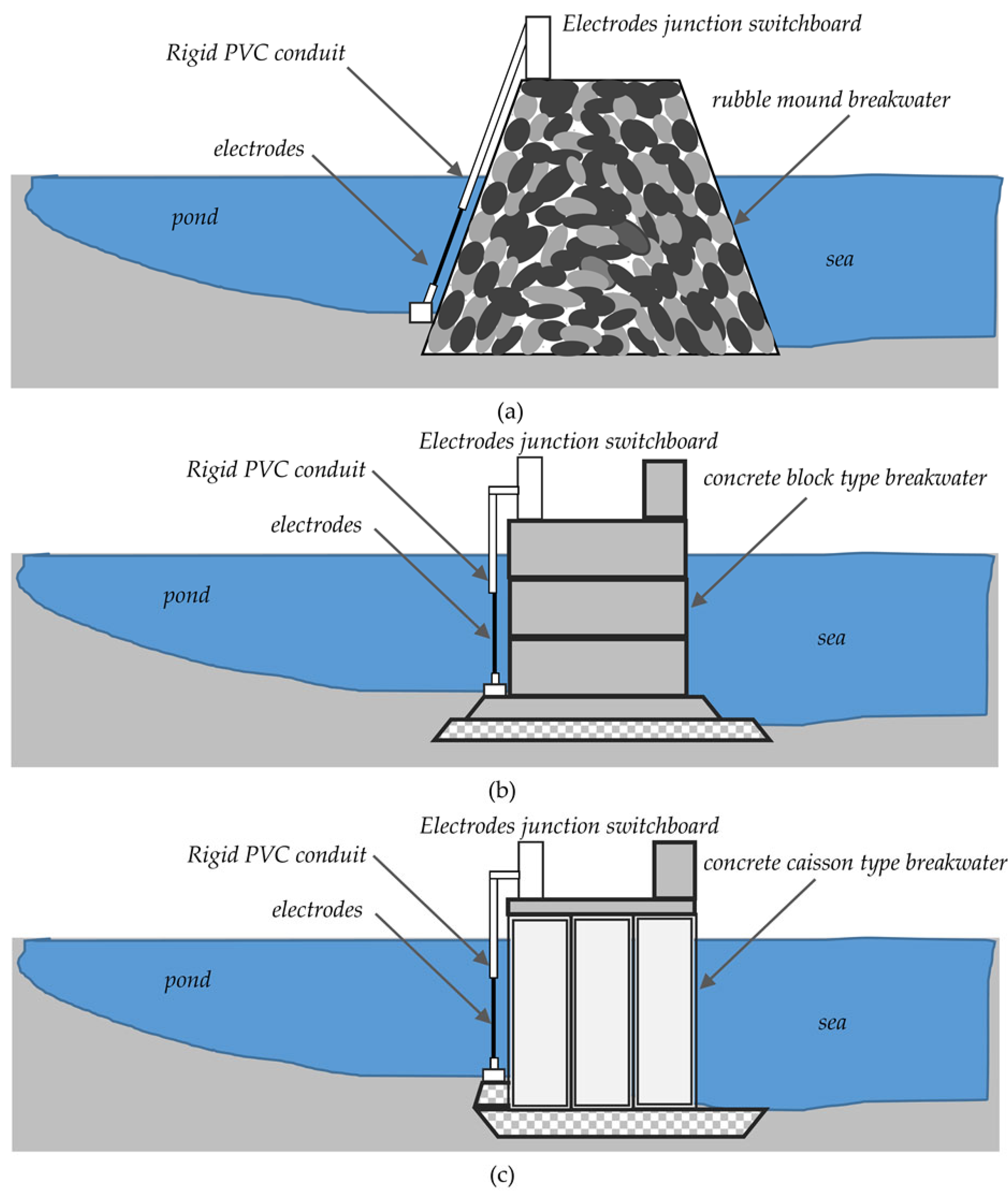
3.1. Breakwater Basic Structure

Based on [78], the relevant literature [1] and the Lower Churchill project [72,73,74] (which in terms of interconnection structure is quite similar to the structure of Crete—Attica), the configuration of coastal electrode stations in Stachtoroi and Korakia was initially proposed, with the formation of a pond and either a rubble mound breakwater (see Figure 10a), a concrete-block one (see Figure 10b) or with concrete caissons (see Figure 10c). The rubble mound breakwater, due to the openings between the rubble, acts as a filter and allows the renewal of water within the pond, while for the other two cases, this is achieved through appropriate openings.

3.2. Basic Breakwater Layout at Stachtoroi, Attica

The corresponding layout of the electrode station for the area of Stachtoroi islet in the Argosaronic gulf, Attica, Greece, is shown in the plan view of Figure 11.

3.3. Basic Breakwater Layout at Korakia, Crete

The corresponding layout of the electrode station for the area of Korakia beach in Crete is shown in the plan view of Figure 12.

3.4. Technical Features of the Electrode Installation

The technical features of the electrode installation are set by IPTO as follows:
  • Operation mode: Bipolar operation, where the currents between the two poles are theoretically equal and opposite. In emergency situations, the unipolar operation occurs due to a failure of the main pole, where the shoreline pond electrodes are used as a return conductor in cooperation with the corresponding DC medium-voltage protection conductor. In case of failure/maintenance of the converter of either pole, the corresponding pole conductor can be used without utilizing the shoreline pond electrodes;
  • Nominal current intensity at monopolar operation: 1,000 A, as each pole has a nominal power of 500 MW under a nominal voltage of 500 kV;
  • Imbalance current intensity at bipolar operation: 11–25 A, since it is not possible to achieve absolute synchronization between the AC/DC converters located at each conversion station, and there is a very small (asymmetrical) current, which flows through the electrodes in their normal operation and does not exceed 1–2% of the nominal current intensity of the converters;
  • Maximum short-time current intensity, under overload conditions: 1,100 A, (i.e., +10% of nominal). Sizing of the electrodes for continuous operating conditions, as well as respective operation effects, were performed with this value;
  • Maximum transient fault current intensity: peak value of 12,800 A at a maximum duration of 0.5 s, as required to clear the fault, due to the use of a voltage source converter;
  • Lifetime of the technical project: 50 years;
  • Economic lifetime: 25 years for electromechanical projects and 50 for civil engineering projects;
  • Load factor at monopolar operation: No data are given, while in itself, it is a very complex problem because the load demand from the Attica–Crete interconnection depends, to a significant extent, not only on the load demand estimates but also on the penetration of R.E.S. in Crete, from the moment this interconnection is made. In the present case, the worst possible factor is assumed (i.e., 1);
  • Transmission line reliability and availability–forced pole outage rate: According to CIGRE guideline 379 [80] (Table 11, p. 11 and Table 30, p. 66), the expected number of failures is 22 in 50 years or 0.433 failures per year;
  • Time interval of forced pole outages and time interval of scheduled pole outages for maintenance reasons: In [78], an aggregate estimation is given that the duration of restoration and maintenance of one of the two poles amounts to 3 months every 5 years, without any additional data;
  • Annual electrode operational duty in Ah: Assuming that the electrode station operates 3 months per 5 years at a maximum short-time current intensity of 1,100 A at monopolar operation and the rest time period at an imbalance current intensity of 25 A at bipolar operation, the average annual electrode operational duty is equal to 646,050 Ah;
  • Electrode station operation, during installation and commission acceptance: During these phases, it is not expected to operate under the IPTO guidelines;
  • Reliability: The configuration of the electrode station is performed in such a way that the necessary electrodes are divided into ν sections, with a reserve of ν + 1. In the present case, the IPTO requirement is ν = 5 so as to achieve a reserve of 20%;
  • Polarity: The polarity of each earth electrode is fully reversible due to the possibility of power flow from Attica to Crete and vice versa, as well as due to the structure of the high voltage DC transmission system, where the flow of asymmetry current and monopolar operation current can reverse the operating polarity of the electrodes;
  • Electrode Materials: IPTO recommends the use of high-silicon iron electrodes of the tubular form (indicatively by ANOTEC, Centertec Z series), conforming to ASTM A518 G3. Silicon content 14.20% ÷ 14.75%, chromium 3.25 ÷ 5.00%, carbon 0.70÷1.10%, manganese up to 1.50%, copper up to 0.50%, molybdenum up to 0.20% and the rest iron. The electrode is cast in a cooled die, with zinc connection in the center of the tube, with mechanical stress resistance equivalent to 1,000 kg, connection resistance of 1 mΩ, type 4884 SZ, weight 143 kg, diameter 122 mm (=2∙rel) and length 2130 mm (=Lel) [77]. In order to achieve reversible operation of the electrode, according to the manufacturer, the electric current density must be limited to 20 A/mm2.
In addition, to determine the interactions and environmental impacts in each area, the following information is required:
  • Seawater electrical resistivity: It generally depends on several factors, such as its salt content–salinity, the depth of the sea, the season, climatic conditions (e.g., prevailing temperatures) and so forth. From measurements carried out by the Hellenic Marine Research Centre, the following data were obtained regarding the seawater at Stachtoroi (Attica) and Korakia (Crete) areas:
    Salinity: The water salinity value varies:
    For the area of Stachtoroi, 38 ÷ 39 psu (practical salinity units or ‰ content), in water temperatures of 24 ÷ 29 °C, to a depth of approximately 90 m;
    For the area of Korakia, 38.9 ÷ 39.6 psu (practical salinity units or ‰ content), in water temperatures of 24 ÷ 26 °C, to a depth of approximately 90 m.
    Electrical resistivity: It takes the value of 0.167 ÷ 0.212 Ω∙m, which means seawater is a medium of very good conductivity.
Therefore, in the present study, the seawater’s electrical resistivity took a value of 0.25 Ω∙m. In the case of breaking water (water foaming on the shore, jetties, etc., due to the air contained within and at a completely local level of a few meters from the shore or jetty), the respective value can be taken as equal to 2.0 Ω∙m:
  • Soil electrical resistivity: It is roughly determined through the types of soil, since at Korakia, there is slate, with an electrical resistivity of 20 and 1,000 Ω∙m, and at Stachtoroi limestone, with a value of 1,000 to 10,000 Ω∙m, as long as it does not have sediments. The seabed consists, in the best-case scenario, of sandy saline materials with an electrical resistivity that is estimated to be two orders of magnitude greater than that of seawater, i.e., about 10 Ω∙m [81], and in the worst-case scenario, of rocks, with an electrical resistivity that is estimated at least at three to four orders of magnitude greater than that of seawater, i.e., >1,000 Ω∙m [81]. In other words, the seabed is a path with a much higher electrical resistivity than seawater, so for the sake of saving time and financial resources, it is suggested, at the level of a preliminary study, not to measure electrical resistivity at minor and great depths;
  • Soil thermal characteristics of soil: No measurements are needed concerning these characteristics since the electrodes are immersed in the sea;
  • Marinelife around the electrodes: There is no special type of marine fauna and flora in the electrode area other than protected birds at Stachtoroi and Posidonia Oceanica meadows (marine plants) near Korakia;
  • Salinity reduction due to freshwater inflow to seawater: In the area of Stachtoroi, due to the small area of the islet, there is no question of changing the seawater salinity from the overflow of rainwater on the islet after rainfall. In the area of Korakia, two small dry rivers end in the small bay (as shown in Figure 12), which are not expected to cause a substantial change in seawater salinity from the runoff of rainwater as they are not rivers or underground sources of constant or significant flow. Moreover, the “rounding-up” of the seawater electrical resistivity to 0.25 instead of the maximum 0.212 Ω∙m leaves a significant reserve margin, in case of changes in the electrical resistivity.

4. Application of Electric Field Distribution Methods Using an Equivalent Electrode

4.1. General Remarks

Any method based on an equivalent electrode through which all electric current flows is suitable for the determination of the electric field in the case of the far field. The method based on a linear current source is suitable for the calculation of the near electric field, but it is not suitable for the far field. This method is presented only for comparison purposes. In order to study the far-field distribution at each electrode station, nearby areas with houses or industries were studied. In the case of Stachtoroi, four characteristic areas were studied: Aegina, whose nearest coast with houses is at 7.8 km, as shown in Figure 2; Salamina at 9.5 km; Pachi-Megara at 17.5 km; and the natural gas unit at Revythousa at 16.4 km. The corresponding maximum depths and angles are given in Table 1. The exposed side to the sea near the coast is limited to 150°, while if one moves away from the island, it widens well beyond 180°. The corresponding correction factor for the electric field distribution method according to CIGRE B4.61 675:2017 and IEC TS62344:2013, as well as for the modified one with the addition of a dam, is 180°/150° = 1.20, very close to shore and less than 1 if one goes beyond 50 m from an electrode placement point. Therefore, in this case, no correction factor was necessary. In the case of Korakia, the nearest opposite coast is over 110 km on the island of Santorini. However, on the island of Crete, at a distance of about 1.5 km from the coast, there are seaside buildings, while at 0.8 km on land, there are farms. The exposed side towards the sea near the shore is limited to 112°, while, further away, it widens over 180°, according to Figure 3. Very close to shore, the corresponding correction factor is 180°/112° = 1.60, while 100 m away from an electrode, it is about 1. In this study, a correction factor of 1.30 was set. Table 1 lists the respective depth and angle values θw at near distances (50 m) and long distances (20 km). In addition, in both areas under study, it is considered that the ground has a small elevation in relation to the variations in the sea depth. Consequently, it can be considered as horizontal, i.e., θs = π-θw, approximating better the IEC standard TS62344:2013.

4.2. Application of Method “A”—Combination of Electric Field Distribution Methods by CIGRE B4.61 675:2017 and IEC TS 62344:2013

Applying the combination method of electric field distribution according to CIGRE B4.61 675:2017 and IEC TS 62344:2013 in the area of Stachtoroi, the results for the worst-case scenario, i.e., with infinite soil resistivity, and for the scenarios with the smallest and the highest possible electrical resistivities (ρs = 1,000 Ω·m and ρs = 10,000 Ω·m) are presented in Table 2. It is found that the worst-case scenario and the scenario with the highest possible electrical resistivity give very similar results. In addition, for the worst-case scenario, the voltage is smaller than 4 V before reaching any residential shore, comparing the limit rlimit1 to the corresponding distances in Table 1. Moreover, the electric field strength is limited to 1.25 V/m in a radius of 153 m from the position of the point electrode. In the case of the transient phenomenon, the distances are slightly shorter.
Similarly, by applying the corresponding method in the area of Korakia, the results for the worst-case scenario, i.e., with infinite soil resistivity, and for the scenarios with the smallest and the highest possible electrical resistivities (ρs = 100 Ω·m and ρs = 1,000 Ω·m) are presented in Table 3. The initial values of Equations (8) and (9), (74), (76) and (77) were recorded, as well as after the implementation of the correction factor 1.30, where the respective values are increased. It was found that the scenario with the highest possible electrical resistivity gives slightly improved results compared to the worst-case scenario due to the fact that the resistivity is set at 1,000 Ω·m. However, even for the worst-case scenario, the voltage is smaller than 4 V at a distance of 1,200 m (shorter distance than the distance to existing structures, roads, etc.). Only in the south–southeast is there an arable area without buildings at a distance of 850–1,200 m. In this area, no effects are expected because the voltage is smaller than 1.18 V at a distance of 350 m. The electric field strength is limited to 1.25 V/m for a radius of 70 m from the position of the point electrode (due to the effect of a near field, the exact position of the electrode must be taken into account). In the case of the transient phenomenon, the distances are slightly shorter.
The indicative value of the resistance of the electrode station in relation to remote earth for the worst-case scenario is extremely high in both cases (432 Ω for Stachtoroi and 67 Ω for Korakia, i.e., a total of 542 Ω). This value does not represent reality, as it was assumed that the whole electric current passes through an electrode with a radius of 0.061 m and with extremely high potential (475 kV for Stachtoroi and 73.3 kV for Korakia). The use of non-infinite values of resistivity improves the corresponding quantities by up to 21%, which, however, remain at high levels. The above data show that the method proposed by CIGRE B4.61 675:2017 and IEC TS 62344:2013 gives results of quite higher values, rendering the design more difficult.

4.3. Application of Method “B”—Combination of Electric Field Distribution Methods by CIGRE B4.61 675:2017 and IEC TS 62344:2013 (Modification Taking the Dam into Consideration)

By applying the modified method of electric field distribution according to CIGRE B4.61 675:2017 and IEC TS 62344:2013 with the addition of a dam in the area of Stachtoroi, it was assumed that the thickness of the dam is 16.0 m at a distance of 1.0 m from the electrode (r1 = 1.0 m, r2 = 17.0 m). Six scenarios were considered involving all possible combinations using infinite soil resistivity, the smallest and highest possible resistivities (ρs = 1,000 Ω·m and ρs = 10,000 Ω·m) and using the smallest and highest possible electrical resistance of a rubble mound or concrete dam with gaps filled with seawater (ρd = 100 Ω·m and ρd = 120 Ω·m).
The safety distances rlimit1 for voltage Vlimit_S, rlimit2 for a steady-state mean value of electric field strength Elimit_S, rlimit3 for a transient mean value of electric field strength Elimit_Τ, rlimit4 for the steady-state point value of electric field strength Elimit_S, and rlimit5 for the transient point value of electric field strength Elimit_Τ present no variations compared to the values in Table 2, because the corresponding distances are located outside the dam, and are therefore not affected by the dam resistivity. On the contrary, the values of the electrode station resistance and the corresponding high absolute potential are significantly increased due to the addition of the dam, as shown in Table 4. When the effect of the soil is ignored, the values are 23.9 times higher than the corresponding values of method “A” for dam resistivity ρd = 100 Ω·m, while, if the soil is taken into account, the variations are between 1.35 and 5.85 times higher achieving the smallest differences for the smallest possible soil resistivity and the widest angles θw. If the dam resistivity is increased by 20% (ρd = 120 Ω·m), then in the worst-case scenario (ignoring the soil effect), there is an increment of 19.2%, while when the soil effect is taken into account, then it is limited from 0.1% to 3% for resistivities ρs from 1,000 to 10,000 Ω·m.
With the addition of a rubble mound dam in the area of Korakia, the assumption that the thickness of the dam is 18.0 m at a distance of 1.0 m from the electrode, i.e., r1 = 1.0 m, r2 = 19.0 m, is made. Six scenarios were considered, including all possible combinations using infinite soil resistivity, the lowest and highest possible soil resistivity (ρs = 100 Ω·m and ρs = 1,000 Ω·m) and using the lowest and highest possible resistivity of a rubble mound dam with seawater-filled gaps (ρd = 100 Ω·m and ρd = 120 Ω·m). The values of the respective safety distances rlimit1, rlimit2, rlimit3, rlimit4 and rlimit5 are the same compared to the values in Table 3. On the contrary, the values of the electrode station resistance with respect to remote earth and the corresponding high absolute potential increase significantly due to the addition of the dam, as shown in Table 5. Ιgnoring the soil effect, the values are 24.1 times higher than the corresponding values of method “A” for the case of dam resistivity ρd = 100 Ω·m, while, if the soil is taken into account, the variation is limited between 1.29 and 4.75 times higher achieving the smallest differences for the smallest possible soil resistivity. If the dam resistivity is increased by 20% (ρd = 120 Ω·m), then in the worst-case scenario, by ignoring the soil effect, there is an increment of 19.2%, while when the soil effect is taken into account, then it is limited from 0.1% to 2.2% for the electrical resistivities ρs from 100 to 1,000 Ω·m.
Of course, in both cases examined (Stachtoroi and Korakia), the values of the resistance of the electrode station with respect to remote earth for the worst-case scenario are extremely high, much higher than those of method “A”. This is not the actual case, as it was assumed that all the current intensity passes through an electrode of a radius of 0.061 m and that this electrode is also surrounded by a high resistivity dam of thickness d (16 m for Stachtoroi and 18 m for Korakia) and by the soil of infinite resistivity. The use of non-infinite resistivity values regarding the soil improves the respective values by up to 95%, which, however, remain at high levels. The modified point source method by CIGRE B4.61 675:2017 and IEC TS 62344:2013 with the addition of a dam eventually gives quite unfavorable results, especially regarding the resistance of the electrode station with respect to remote earth and the corresponding developed absolute potential.

4.4. Application of Method “C”—Near Electric Field Distribution Method with Linear Current Source

By applying the near electric field distribution method, with a linear current source and with the addition of a rubble mound breakwater, the inclination of the seabed and of ground is not used, but the water zone of height/active electrode length L. In the case of a rubble mound breakwater with an inclination λ (base:height), as in Figure 10a, the water zone L is determined through the geometric length of the electrode Lel equal to:
L = L e l × c o s a t a n λ
If the electrode is placed vertically, as in Figure 10b,c, then L = Lel.
In the case of Stachtoroi, based on Figure 11, the angle θ of the top view of Figure 6 is 210°, and the thickness of the dam at the point where the electrode is placed is 16.0 m, so the radius r2 is equal to 17.0 m, while the radius r3 (for which it is ensured the same depth as the lower end of the electrode, along the entire length of the dam) is equal to 10.0 m. The sea distance between the two electrode stations is equally divided, thus setting r equal to 150 km. The rubble mound breakwater inclination λ amounts to 3:2, so the respective electrode inclination is the same; thus, the active length L of the ANOTEC electrode (see Section 3.4) is equal to 1.1815 m. In the case of a special composition concrete breakwater, the electrode is placed vertically with a respective active length of 2.13 m. Similar to the application of method “B”, the six scenarios are examined, which include all possible combinations, using three soil electrical resistivity and two breakwater electrical resistivity values for the two different active electrode lengths (3:2 inclination and vertical). Table 6 lists the respective results. In the case of the 3:2 electrode inclination, it is found that the voltage drops below 4 V, with respect to “infinity”, at 143.5 km, which fully displays the inability to describe the far field since it studies only a narrow water zone, equal to the active length L (=1.1815 m). However, the electric field strength below 1.25 V/m is limited to a radius of 71 m from the position of this linear electrode. In the case of the transient phenomenon, slightly shorter distances result. Effect of the electrical resistivity of the breakwater material does not exist at the distance limits because they lie beyond the breakwater area and is limited to large soil electrical resistivities, increasing the maximum electrode resistance to remote earth from 16.0 Ω to 21.5 Ω, and the absolute potential on the electrode from 17.6 kV to 23.7 kV. Here, the effect of the linear electrode on the calculation of the electrode resistance to remote earth and on the voltage on the electrode is additionally observed, as there is a significant reduction compared to the results of Table 2 and Table 4. Therefore it seems that beyond the distance of the far-field effects (where the model’s failure was expected from the start), in the remaining quantities, it gives values that represent the near field much better. Additionally, if the electrode is placed vertically and not with a 3:2 inclination, with a suitable suspension device, then a significant reduction in the electric field strength is observed, below 1.25 V/m, as it is limited to a radius of 40 m from the position of the linear electrode, for an active length of 2.13 m, which basically states—in relation to the 16 m breakwater thickness—that at an external distance from the breakwater, of the order of 23 m, there will be no problem for swimmers and sea creatures/mammals, dropping at 26% of the value of methods “A” or “B”. Moreover, significant reductions occur regarding the maximum electrode resistance to the remote earth (dropping to 12.0 Ω) and absolute potential across on electrode (to 13.1 kV), even for infinite soil electrical resistivity.
Respectively, in the case of Korakia, based on Figure 12, the angle θ of the plan view of Figure 6 is 245°, and the thickness of the breakwater at the electrode position is 18.0 m, so the radius r2 is equal to 19.0 m, while the radius r3 is equal with 25.0 m. The rest of the geometric features are the same as those at Stachtoroi. Similar to the application of method “B”, the six scenarios are examined, which include all possible combinations, using three soil electrical resistivity and two breakwater electrical resistivity values for the two different active electrode lengths (3:2 inclination and vertical). Table 7 lists the respective results. In the case of the 3:2 electrode inclination, it was found that the voltage drops below 4 V, with respect “infinity”, at 145 km, which fully displays the inability to describe the far-field since it studies only a narrow water zone, equal to the active length L (=1.1815 m). However, the electric field strength, below 1.25 V/m, is limited to a radius of 93 m from the position of this linear electrode. In the case of the transient phenomenon, slightly shorter distances result. Effect of the electrical resistivity of the breakwater material does not exist at the distance limits because they lie beyond the breakwater area and is limited to large soil electrical resistivities, increasing the maximum electrode resistance to remote earth from 1.161 Ω to 1.166 Ω, and the absolute potential on the electrode from 1.277 kV to 1.283 kV. Here, the effect of the linear electrode on the calculation of the electrode resistance to the remote earth and on the voltage on the electrode is additionally observed, as there is a significant reduction compared to the results in Table 3 and Table 5. Therefore it seems that beyond the distance the far field affects, in the remaining quantities, it gives values that represent the near field much better. Additionally, if the electrode is placed vertically with a suitable suspension device, then a significant reduction in the electric field strength is observed, below 1.25 V/m, as it is limited to a radius of 51.5 m from the position of the linear electrode for an active length of 2.13 m, which basically states—in relation to the 18 m breakwater thickness—that at an external distance from the breakwater, of the order of 32 m, there will be no problem for swimmers and sea creatures/mammals, dropping at 76% of the value of methods “A” or “B”. Respectively, significant reductions occur regarding the maximum electrode resistance to remote earth (dropping to 0.65 Ω) and absolute potential across on electrode (to 0.71 kV), even for infinite soil electrical resistivity.
From the study of the two cases (Stachtoroi and Korakia), in terms of the effect of the values of the electrical resistivities of soil and breakwater, there are no large differences despite their range of values. This is due to the low seawater electrical resistivity and the water zones formed. On the contrary, the active length of the electrode has a significant effect, leading to significantly improved results.
The data above demonstrate that the proposed model is suitable for the near field since the electrode is considered a linear rather than a point source. On the contrary, due to the assumption of a constant conduction zone of constant depth, much smaller than that in which the electric current is diffused over long distances, it is unsuitable for the far field.

4.5. Comparison of Methods and Combined Utilization

In order to compare the proposed methods, the corresponding results of the electric field strength, with respect to the distance from the one concentrated electrode, for the case of Stachtoroi, Attica, are presented in detail. The geometric dimensions of the layout of Figure 4 and Figure 6 are the following: θw = 0.2718° = 0.004743554 rad (the worst-case scenario concerning Aegina in Table 1), θ = 210°, r1 = 1.0 m, r2 = 17.0 m, r3=10.0 m, r = 150 km. The electrical resistivity of the soil amounts to ρs = 1,000 Ω·m and of the rubble-mound or concrete with seawater-filled gaps breakwater to ρd = 100 Ω·m. Figure 13 shows the change in the electric field strength on a semi-logarithmic scale in relation to the distance of up to 150 km since, on a linear scale, the respective changes would not be easy to read. It can be seen that, for long distances, the “C” method of the linear current source gives much higher electric field strength values, as it disregards the seabed slope and the increasing depth of the seawater, which reaches up to 37 m, remaining at a layer of water of constant thickness of 1.1815 m. Additionally, the results of methods “A” and “B” are identical.
Figure 14 shows the respective distribution of the electric field strength within the area of the breakwater (i.e., for distances between rel and r1), resulting in the values of methods “A” and “B”, by using a point current source, being identical and giving much higher values than method “C” and much less approximate the near field behavior. This is reinforced by the results of Figure 15 for the electric field strength in the breakwater area, where the values are extremely high due to the breakwater electrical resistivity. This demonstrates the weakness of the original “A” method, of electric field distribution, according to CIGRE B4.61 675:2017 and IEC TS 62344:2013, which does not take the breakwater into account. However, method “B”, also leads to very high values, at close distances, due to the use of a point source. On the contrary, it is at this point that method “C” of electric field strength distribution is advantageous by using a linear current source, which better approximates reality, giving smoother changes in electric field strength. In particular, the area between the distances r3 = 10.0 m and r2 = 17.0 m gives high values due to the existence of only soil and breakwater. From Figure 16, which concerns a water area outside the breakwater, it is clearly seen that method “C” of the linear current source gives smaller electric field strength values at close distances, utilizing, in essence, the larger water zone, with respect to methods “A” and “B”, whose results are identical, but use a small seawater wedge of angle θw. This is attenuated at longer distances since Figure 17 demonstrates that at about 240 m and beyond, the results are identical. Of course, for very long distances, the values of methods “A” and “B” provide more favorable results (as was seen in Figure 13), as the seawater wedge, of angle θw, grows larger than the horizontal layer of water, defined by method “C” of the linear power source.
Therefore, method “C” of the linear current source is recommended within the breakwater area, inside the breakwater, and on the outer area, for up to the distance rC→A, beyond which method “A” (or “B”, since in that region they are identical) of the point current source, gives smaller values of electric field strength, as the wedge of seawater of angle θw better approximates the seawater mass than does the limited horizontal water layer, defined by the method “C” (of the linear current source) at long distances. The smooth transition between the two methods takes place at a distance where the respective electric field strengths of methods “A” and “C” (for the external area of the breakwater) are equal. Therefore, by equalizing Equations (7) or (23) and (44), the distance rC→A results as equal to:
r C A = L 2 × 2 × π θ ρ w + θ ρ s θ w ρ w + θ s ρ s × c f
where cf is the correction factor of the electric field strength, due to limited exposure of a point electrode to the sea, at an angle φ, smaller than 180° by methods “A” and “B”, equal to π/φ, where φ expressed in rad. In the case of Stachtoroi, the correction factor is 1.0, while in the case of Korakia, it is 1.3. In both cases, the angle of the soil layer θs is equal to 2 × π-θw in Figure 4 or Figure 5.
Therefore, to calculate the safety distances rlimit2, for an average value of electric field strength Elimit_S (continuous operating conditions); rlimit3, for an average value of electric field strength Elimit_T (transient operating conditions); rlimit4, for a point value of electric field strength Elimit_S (continuous operating conditions); and rlimit5, for a point value of electric field strength Elimit_T (transient operating conditions), it is suggested to use the method “C”, of the linear current source, due to its suitability for short distances (of the order of tens of meters). On the contrary, for the calculation of the safety distance rlimit1 for voltage Vlimit_S, with respect to infinity, it is recommended to use method “A” (or “B”, since in that area they are identical) due to its suitability for long distances (of the order of a few km).
For the calculation of electric field strength, the absolute potential on the surface of an electrode, with respect to infinity (remote earth), and the equivalent electrode station resistance, the combined application of the methods was proposed. More specifically, method “C” of electric field strength distribution, through a linear current source and a water zone of constant thickness, was applied from the surface of the electrode up to the distance where the electric field strengths of methods “A” and “C” are equalized (i.e., rel < r < rC→A), whereas the unified method “A”, of electric field strength distribution through a point current source, according to CIGRE B4.61 675:2017 and IEC TS 62344:2013, was applied from the distance where the electric field strengths of methods “A” and “C” are equalized, towards infinity (i.e., rC→A < r < ∞). From the calculation of the electric field strength, the absolute potential, with respect to infinity (remote earth), can be calculated and, subsequently, the respective equivalent electrode resistance. Hence, for the case of Stachtoroi, Attica (since r1 < r3 < r2 < rC→A), according to Equation (83), the absolute potential is calculated as follows:
V r = r r E × d = r r 1 E × d Equation   46 + r 1 r 3 E × d Equation   49 + r 3 r 2 E × d Equation   52 + r 2 r C A E × d Equation   44 + r C A E × d Equation   8
V ( r ) = ρ w × I t o t 2 × π × L × l n r 1 r + I t o t L × 2 × π θ ρ d + θ ρ w × l n r 3 r 1 + I t o t L × 2 × π θ ρ d + θ ρ s × l n r 2 r 3 + I t o t L × 2 × π θ ρ w + θ ρ s × l n r C A r 2 + I t o t × c f 2 × r C A × θ w ρ w + θ s ρ s : r < r 1 I t o t L × 2 × π θ ρ d + θ ρ w × l n r 3 r + I t o t L × 2 × π θ ρ d + θ ρ s × l n r 2 r 3 + I t o t L × 2 × π θ ρ w + θ ρ s × l n r C A r 2 + I t o t × c f 2 × r C A × θ w ρ w + θ s ρ s : r 1 < r < r 3 I t o t L × 2 × π θ ρ d + θ ρ s × l n r 2 r + I t o t L × 2 × π θ ρ w + θ ρ s × l n r C A r 2 + I t o t × c f 2 × r C A × θ w ρ w + θ s ρ s : r 3 < r < r 2 I t o t L × 2 × π θ ρ w + θ ρ s × l n r C A r + I t o t × c f 2 × r C A × θ w ρ w + θ s ρ s :   r 2 < r < r C A I t o t × c f 2 × r × θ w ρ w + θ s ρ s :   r > r C A
Accordingly, the electrode station resistance of remote earth results from Equation (85) (for r = rel < r1) as follows:
R e l = V r e l I t o t = 1 L × l n r 1 r e l 2 × π ρ w + l n r 3 r 1 2 × π θ ρ d + θ ρ w + l n r 2 r 3 2 × π θ ρ d + θ ρ s + l n r C A r 2 2 × π θ ρ w + θ ρ s + L × c f 2 × r C A × θ w ρ w + θ s ρ s
If the inequality r1 < r3 < r2 < rC→A does not apply, then it is examined whether the inequality r1 < r3 < rC→A < r2 is valid, determining the equalization distance of the electric field strengths of methods “B” and “C”, through Equations (26) and (52), hence it follows that:
r C A = L 2 × 2 × π θ ρ d + θ ρ s θ w ρ d + θ s ρ s × c f
Here, method “B” is necessarily used instead of method “A”, since the respective distance lies on the breakwater. Consequently, the absolute potential is calculated, similarly to Equation (85), and from this, the electrode station resistance of remote earth results as equal to:
R e l = 1 L × l n r 1 r e l 2 × π ρ w + l n r 3 r 1 2 × π θ ρ d + θ ρ w + l n r C A r 3 2 × π θ ρ d + θ ρ s + L × c f 2 × θ w ρ w + θ s ρ s × 1 r C A 1 r 2 + L × c f 2 × r 2 × θ w ρ w + θ s ρ s
It is noted that the equalization distance of the electric field strengths of methods “A” and “C” by applying Equation (83) is greater than that resulting from applying Equation (86) under the practical condition that the electrical resistivity of the soil ρs is much greater than the respective seawater ρw. In particular, the corresponding condition for θs = 2×π-θw is (2 × π-θ)/θ < ρw/ρs, which is practically the case.
Likewise, for the case of Korakia, Crete, if it is true that r1 < r2 < r3 < rC→A, where the equalization distance of the electric field strengths of methods “A” and “C” (for the external area of the breakwater) results from Equation (83), then the absolute potential is calculated in a similar way and from this electrode station resistance of remote earth results as equal to:
R e l = 1 L × l n r 2 r 1 2 × π θ ρ d + θ ρ w + l n r 3 r 2 × r 1 r e l 2 × π ρ w + l n r C A r 3 2 × π θ ρ w + θ ρ s + L × c f 2 × r C A × θ w ρ w + θ s ρ s
If the inequality r1 < r2 < r3 < rC→A does not apply, then it is examined whether the inequality r1 < r2 < rC→A < r3 is valid, determining the equalization distance of the electric field strengths of methods “A” or “B” and “C”, through Equations (7) or (23) and (46), hence it follows that:
r C A = L × π ρ w θ w ρ w + θ s ρ s × c f
Consequently, the absolute potential is calculated, similarly to Equation (85), and from this, the electrode station resistance of remote earth results as equal to:
R e l = 1 L × l n r 1 r e l × r C A r 2 2 × π ρ w + l n r 2 r 1 2 × π θ ρ d + θ ρ w + L × c f 2 × r C A × θ w ρ w + θ s ρ s
It is noted that, if during the calculation of the equalization distance of the electric field strengths of methods “A” and “C”, by applying Equation (83), the condition r1 < r2 < rC→A < r3 is met, instead of r1 < r2 < r3 < rC→A, and, respectively, by applying Equation (89), the condition r1 < r2 < r3 < rC→A is met, instead of r1 < r2 < rC→A < r3, then distance r3 is considered the corresponding equalization distance of the electric field strengths of methods “A” or “B” and “C”, at which the strength of the electric field presents a discontinuity.
Each case, different from those of Stachtoroi and Korakia, should be examined, particularly in terms of finding analytical relations because due to the numerical values (regarding distances r1, r2, r3 and rC→A), different equations could result in calculating the absolute potential (with respect to infinity) and the electrode station resistance (with respect to remote earth), but corresponding to those resulting from Equations (84) and (85).
In the present case, from the relevant calculations, for the most unfavorable conditions of Stachtoroi and Korakia, the respective results of Table 8 were obtained. From the comparison of the results with the corresponding ones in Table 6 and Table 7, a small improvement between 1.7% and 2.7% was observed for the area of Stachtoroi, and a great one between 60% and 68% for the area of Korakia. This occurs because the equalization distance of the electric field strengths between methods “A” or “B” and “C”, in the case of Korakia, is much shorter compared to that of Stachtoroi, which is mainly attributable to the much greater seabed slope used in methods “A” and “B”. However, the total equivalent electrode station resistance, with respect to remote earth, has been significantly reduced compared to the values determined either by method “A” (smaller by 20 to 100 times) or by method “B” (smaller by 1,000 to 2,000 times). Even under the worst-case scenario, for a 3:2 inclination of the electrode, the total resistance of the two electrodes through remote earth amounts to 21.5 Ω and the potential difference between them to 23.69 kV, while for a vertical electrode, it is further reduced to 12.0 Ω and at 13.21 kV, respectively, demonstrating the superiority of the combined use of methods “A” or “B” and “C” to determine an upper limit in terms of the absolute potential on an electrode surface, as well as in terms of the equivalent electrode station resistance, with a relatively easy analytical mathematical procedure of direct calculation.
Regarding the safety distance from the breakwater, the use of method “C” was proposed, with the relevant results as analyzed in Section 4.4, where the most unfavorable results in the present cases result from the activation of the limits of the electric field strength at steady state (see Table 6 and Table 7). On the contrary, the minimum distance, regarding absolute potential with respect to remote earth at a steady state, was achieved through methods “A” or “B”, where for Stachtoroi, it was located outside all inhabited areas, whilst for Korakia, it was limited to a distance of 1.12 km from the electrode station, even for the most unfavorable combination of geometric dimensions and electrical resistivities.

5. Application of Electric Field Distribution Methods Using Superposition for Near Field Analysis

5.1. General Remarks

As already mentioned in Section 2.4, in this study, an ANOTEC electrode [77] was chosen, and it was suggested by IPTO that the electric current density limit value Jst be equal to 20 A/m2, while for reliability reasons, the number of linear frames vframe be 5 with an additional reserve of 1. Thus, for a total electric current intensity Ιtot_steady, at a steady state (under overload conditions) equal to 1,100 A from the application of Equation (59), it follows that the number of necessary electrodes Nmin_el is equal to 67. Therefore, by applying Equation (60), it follows that in each frame, the number of necessary electrodes Nel_frame is 13, while in total (including the reserve frame), 78 electrodes were used.
By taking into account the increment factor β equal to 6.1%, the final values of current densities, under full load conditions Jfull_load_steady and under periodic maintenance conditions Jmaintenance_steady were calculated as equal to 18.33 A/m2 and 22.00 A/m2, through Equations (61) and (62), respectively. Similarly, for the transient state, for a respective current intensity Itot-transient equal to 12.8 kA, the final values of current densities, under full load conditions Jfull_load_transient and under periodic maintenance conditions Jmaintenance_transient are calculated as equal to 213.28 A/m2 and 255.93 A/m2, respectively.
Based on Section 4.4 and Section 4.5, for the study of the electric field distribution at short distances (near the breakwater), the most suitable method is “C” using the linear current source. For the sake of simplifying the calculation process, the effect of the soil (considering its electrical resistivity to be infinite), the water zone of a respective arc of angle θ on the plan view of Figure 6, as well as of the breakwater, were all ignored, therefore from Equations (44), (46), (49) and (52), the electric field strength results as follows:
E r w _ r = ρ w × I t o t 2 × π θ × r × L  
The first two simplifying admissions led to much more unfavorable results, whilst not considering the breakwater only has an effect on the calculation of the electric field strength when one is on the breakwater, as well as on the calculation of the absolute potential for radii within or up to the breakwater (i.e., for r < r2). In the present case, of interest is the electric field strength mainly beyond the breakwater, while regarding the electric field strength on it Εrd_r by simplifying, its value can be approximated by multiplying the respective seawater electric field strength Εrw_r by the ratio of the electrical resistivities ρdw, that is:
E r d _ r = ρ d ρ w × E r w _ r  
Equation (91) was practically applied; for each electrode located at position (x, y) of Figure 9 and through Equations (63) to (68), the superposition theorem was applied to determine the electric field strength resultant, in the case of the frame of Figure 7 and in the case of the array of linear frames placed parallel to the axis of the protective breakwater of Figure 8. Consequently, the relative analysis was made in a step-by-step process, emphasizing the area of Korakia, Crete, considering the arc of the “right” water–breakwater zone (2 × π-θ) of Figure 6 as equal to 112°, which is smaller than the respective arc of 150° at Stachtoroi, in seawater of electrical resistivity of 0.25 Ω∙m. In addition, emphasis is placed on the study of current intensity densities under conditions of periodic maintenance at a steady state because they generally give the most unfavorable results, in terms of safety distance, with respect to the point electric field strength criterion of 1.25 V/m.

5.2. Case of an Electrode at Maximum Electric Current Density, under Periodic Maintenance Conditions

Initially, the study was made of an electrode at a steady state, electrified with a current density of 22 A/m2 (under conditions of periodic maintenance), on a canvas of dimensions 5 m (Ox semi-axis) by 10 m (yOy’ axis), with a step of 0.05 m, in the area of Korakia (with a computational mesh of 101 × 201 = 20,301 points). Due to the 3:2 inclination of the electrode, the effective length L was taken equal to 1.1835 m. Through this simulation, the electric field strength on the Oxy plane (Figure 18), as well as the area of the electric field strength, with values greater than 1.25 V/m (Figure 19), were obtained.
The maximum electric field strength was calculated as equal to 31.87 V/m, which is fully consistent with the respective electric field strength of Equation (91), while the distance where it stays below the limit of 1.25 V/m was determined at 1.555 m. These quantities are significantly improved in relation to those that would be obtained by method “A” (15,091.5 V/m and 6.703 m, respectively). Essentially, this means that there is no electric field strength greater than 1.25 V/m beyond the dam, as the latter has a crest width of at least 4.0 m. Additionally, at a distance of 1.0 m from the electrode, the dam begins, so in this case, the corresponding electric field strength in seawater is equal to 1.9441 V/m, which is equivalent to ρd = 100 ÷ 120 Ω∙m, according to Equation (92), with an electric field strength Εrd_r, on the dam, ranging between 777.64 and 933.168 V/m. Therefore, protection measures need to be taken for step voltage, etc. If the same process is repeated with the electrode vertically suspended, with an effective length L equal to 2.13 m, then the maximum electric field strength is calculated to equal to 17.69 V/m, and the distance where it stays below the limit of 1.25 V/m equal to 0.863 m (i.e., within the area of the dam), while the electric field strength Εrd_r on the dam (1.0 m from the electrode) is between 107.84 and 113.232 V/m (need for protection measures for step voltage, etc.).

5.3. Case of a Frame of 13 Electrodes, at Maximum Current Density, under Periodic Maintenance Conditions

Initially, a straight frame was formed consisting of 13 electrodes, which are at a steady state, electrified with a current density (under periodic maintenance conditions) of 22 A/m2, at a distance Del of 1.0 m from each other. This frame is placed on a canvas of 30 m (Ox semi-axis) by 60 m (yOy’ axis—parallel to the axis of the frame), with a step of 0.05 m, with the 7th electrode placed at point O in the area of Korakia (with a computational mesh of 601 × 1,201 = 721,801 points). Due to the 3:2 inclination of the electrode, the effective length L is taken equal to 1.1835 m. From this simulation, the electric field strength on the Oxy plane (Figure 20), and the area of electric field strength, with values greater than 1.25 V/m (Figure 21), were obtained. The maximum electric field strength Emax was calculated as equal to 37.76 (against the 31.87 V/m that was the case with one electrode) due to the superposition of the electric fields of the 13 electrodes. The distance d1, where it stays below the limit of 1.25 V/m along the Ox axis, was determined at 19.53 m, and the distance d1/ along the Oy axis at 20.91 m, with respect to the beginning of the axes. Given that the frame is placed along the perceived axis yOy’ (i.e., parallel to the dam) with its center at point O (from −6.00 m to 6.00 m), it follows that from the end of the frame, the respective required distance dframes is 20.91 − 6.00 = 14.91 m along the Oy axis, so the required frame length k amounts to 12.0 + 2 × 14.91 = 41.82 m. These sizes are significantly improved compared to the values of the corresponding sizes that would be obtained with method “A” (dframes-A = 50.15 m and Emax-A = 15,152 V/m, respectively). It was also found that, compared to the single electrode (where the required distance would be 1.555 m), here it increases significantly due to the superposition effect of the electric field strengths of the neighboring fields, by approximately ten times, while, as expected, the symmetry around the center of the frame is no longer circular but elliptical.
Then the respective distance between the electrodes and rods Del changes, from 0.20 m to 1.50 m, and the critical electric field strength areas, with values greater than 1.25 V/m, were calculated (in addition to the total frame length Dframe and the maximum electric field strength of the array Emax), via the following:
  • The width of the critical frame zone d1 perpendicular to the dam consisted of 13 electrodes on the semi-axis Ox;
  • The total length of the critical frame zone k on the dam consisted of 13 electrodes (on the yOy’ axis);
  • The area of rectangular zone arrangement that ensures the critical frame zone Sk (taking the width d1 for both sides);
  • The estimated distance between successive frames on the dam that ensures the critical zone for diver dropping for repairs dframes (on yOy’);
  • The estimated total length includes the critical zone of 6 frames t on the dam (on yOy’);
  • The area of the rectangular zone arrangement ensures the critical zone of 6 frames St (taking the width d1 for both sides).
Table 9 lists the results for an effective length of 1.1815 m, with an inclination according to that of the dam, while Table 10 lists the results for an effective length of 2.13 m, with vertical suspension.
From the respective study of the results, the following conclusions emerge:
  • As the electrode spacing increases, so do the necessary length on the dam along the yOy’ axis, k, and the area of the rectangular zone arrangement, which ensures the critical zone of six frames, St, (but not monotonously, since for L = 2.13 m and Del > 1.3 m the area St begins to decrease slowly). On the other hand, the maximum electric field strength Emax decreases slightly, as well as the width of the critical zone (in front of the location of the dam d1) and the estimated distance between successive frames dframes, as can be seen from the results of Table 9 and Table 10;
  • By taking into account that, in order to be able to repair each electrode, a distance of 0.50 m between them is practically required, then the required length of the dam is 96 m for L = 2.13 m, which is greater than the available (about 70 m) according to Figure 12. Of course, if from the beginning the array is allowed to move marginally closer to the coast, with the appropriate deepening and by reducing the distance between the frames to 6.5 m, then the required length reaches 68.5 (=6 × 6 + 5 × 6.5), which is feasible. Additionally, the critical zone of the dam marginally extends outside by 5 m (with a crest width of 5 m and a suspension distance of at least 1 m). With the appropriate vertical suspension arrangement, at 6 m from the inner side of the dam, the electric field strength can be less than 1.25 V/m on the outside;
  • In relation to the results of Table 3, it was found that the equivalent point source of method “A” would require a circular zone of about 52.5 m without the correction factor and 68.2 m with the correction factor, whilst, according to Table 7, the equivalent linear source requires 51.5 m, in contrast to the present case of the frame which requires a zone of 10.9 m along the Ox axis and 23.1 m along the Oy axis (for an electrode spacing of 0.50 m and L = 2.13 m). Respectively, the reserved area for the point source amounts to 8,659 m2 (without a correction factor) and 14,612 m2 (with a correction factor), while for the linear source amounts to 8,832 m2, against 1,895 to 2,370 m2 of the linear frames on the dam.;
  • Based on this consideration, the vertical suspension of the electrodes is more suitable; however, due to the phenomenon of the diffusion of the electric current in the seawater, at a short distance from the frame, the behavior of the inclined electrodes tends to approximate that of the vertical ones.
For the sake of completeness, the same procedure was carried out for the area of Stachtoroi, with θ = 210°, L = 2.13 m and ρw = 0.25 Ω∙m. From the respective change in the electrodes—rod spacing Del, from 0.20 m up to 1.50 m—the values of the respective geometric and field parameters were calculated (which determine the critical areas of electric field strength higher than 1.25 V/m) and listed in Table 11.
From the respective study of the results, the following conclusions emerge:
  • As before, as the electrodes spacing increases, so do the necessary length on the dam, along the yOy’ axis k (monotonously) and the area of the rectangular zone arrangement that ensures the critical zone of six frames St (but not monotonously, as for Del > 1.1 m it begins to decrease slowly). Accordingly, the maximum electric field strength Emax is slightly reduced, along with the width of the critical zone, in front of the location of the dam d1 and the estimated distance between successive frames dframes, as can also be seen from the results of Table 11;
  • The required length of the dam (at least 76.5m) is greater than the available (about 55 m), according to Figure 12. Of course, if from the beginning the array is allowed to move marginally closer to the coast, with the appropriate deepening and by reducing the distance between the frames to 4.5 m, then the required length reaches 58.5 (=6 × 6 + 5 × 4.5), which is feasible. Additionally, the critical zone of the dam marginally extends outside by 2 m (with a crest width of 5 m and a suspension distance of at least 1 m). With the appropriate vertical suspension arrangement, at 3 m from the inner side of the dam, the electric field strength can be less than 1.25 V/m on the outside;
  • In relation to the results of Table 2, it was found that the equivalent point source requires a zone of around 152.3 m without the correction factor; according to Table 6, the equivalent linear source would require 39.5 m, in contrast to the present case of the frame, which requires a zone of 8.0 m, on the Ox axis and 17.6 m, on the Oy axis, for an electrode spacing of 0.50 m and L = 2.13 m. Respectively, the reserved area for the point source amounts to 72,870 m2, and for the linear source, it amounts to 4,901 m2, against 1,070 to 1,325 m2 of the linear frames on the dam.

5.4. Case of an Arrangement of 6 Linear Frames of 13 Electrodes Placed in a Row, Parallel to the Protective Dam, at Maximum Current Density under Normal Operation or Periodic Maintenance Conditions

Initially, an arrangement of six linear frames is formed, each consisting of 13 electrode rods with a distance between rods Del equal to 0.50 m and a total length Dframe equal to 6.00 m. The distance between frames dframes is 6.5 m (against 8.52 m in Table 10), which suggests that the total estimated required length of the protective dam, behind which the array of frames is placed, is 81.5 m (=6 × 6.00 + 7 × 6.5), of which 6.5 m, on either outer side, can be considered onshore to be covered by the plan view of the preliminary study dam of Figure 12. The case of loading the electrode station with the maximum nominal load Itotal-steady equal to 1,100 A is considered, for six-frame or five-frame operation, with respective current densities under full load conditions Jfull_load_steady and under periodic maintenance conditions Jmaintenance_steady, respectively. The entire arrangement is placed on a canvas of 60 m (Ox semi-axis) by 160 m (yOy’ axis—parallel to the axis of the frame) and with a simulation step of 0.10 m by 0.10 m (with a computational mesh of 601 × 1,601 = 962,201 points), as seen in Figure 8. From the corresponding simulation, the result of the data of Table 12, with uniform loading of the six-frame or five-frame electrode station, with the sixth, fifth or fourth frame off, as well as the electric field strength graphs, on the Oxy plane in Figure 22, Figure 23, Figure 24 and Figure 25 and the area of electric field strength, with values greater than Elimit_S = 1.25 V/m in Figure 26, Figure 27, Figure 28 and Figure 29, respectively. The results include the following, depending on the mode of operation:
  • The electric current density Jsteady with respect to the peripheral surface;
  • The width d2 of the electrode station critical zone, perpendicular to the dam (on the xOx’ axis);
  • The length of the electrode station critical zone d3 on the dam above the center of the dam (on the yOy’ axis);
  • The length of the electrode station critical zone d4 on the dam below the center of the dam (on the yOy’ axis);
  • The distance of the lowermost rod of the electrode station b-c, on the dam from the center of the dam that is connected to the power supply (on yOy’);
  • The distance of the uppermost rod of the electrode station u-c, on the dam from the center of the dam, connected to the power supply (by yOy’);
  • The distance between the lowermost rod of the electrode station sb-c on the dam that is connected to the power supply and the nearest point of protection (dam end, electrode not connected to power supply for maintenance purposes);
  • The distance between the uppermost rod of the electrode station su-c on the dam, which is connected to the power supply, and the nearest point of protection (dam end, electrode not connected to power supply for maintenance purposes);
  • The distance yp between the nearest point of protection (dam edge, electrode not connected to power supply for maintenance purposes) from the center of the dam that is connected to the power supply (on yOy’);
  • The safety margin Dyp in relation to an initial preliminary study of a frame under the same conditions (where negative values indicate a requirement for a greater safety distance);
  • The maximum electric field strength of the arrangement Emax.
From the study of the relevant results in Table 12, the following conclusions emerge:
  • The deviation at the ends of the arrangement reaches up to 27.0 m depending on the electrifying method (especially when electrifying five consecutive panels). However, in the area of the frame that does not operate, the respective electric field strength is marginally above 2.5 V/m, so there is no safety issue during maintenance as long as the diver takes the appropriate measures;
  • The deviation of the maximum developing electric field strength of the electrode station against that of a single frame (26.09 V/m against 24.06 V/m) is of the order of 8.4%, which is quite large, but expected, given the fact that, instead of 8.5 m, the distance between of frames decreased to 6.5 m;
  • The critical zone of the dam extends outside the dam by 44 m (with a crest width of 5 m and a suspension distance of at least 1 m) on the xOx’ axis (vertical to the dam), where the initial estimation of Table 10 has failed;
  • The critical zone of the dam extends beyond the dam by 66 m (33 m on either side) on the yOy’ axis (parallel to the axis of the dam) in the shore area. The reason is that the distance between the frames was significantly reduced.
If the previous procedure is repeated, setting the intermediate distance between the frames at 8.5 m, according to Table 10, the total estimated required length of the protective dam behind which the array is placed must be 95.5 m (=6 × 6.00 + 7 × 8.5), of which 8.5 m on either outer side can be considered on the coast. From the corresponding simulation, the results of Table 13 are obtained, from the study of which the following conclusions are drawn:
  • The deviation at the ends of the electrode station reaches up to 23.0 m depending on the electrifying method (especially when electrifying five consecutive panels). However, in the area of the frame that does not operate, the respective electric field strength is marginally above 2.5 V/m, so there is no safety issue during maintenance;
  • The deviation of the maximum developing electric field strength of the electrode station against that of a single frame (25.84 V/m against 24.06 V/m) is of the order of 7.4%, which is quite large, despite the fact that the distance between frames is 8.5 m, as set from the beginning. This happens because, in method “C”, the constant effective length causes the field effect to decrease more slowly;
  • The critical zone of the dam extends outside the dam by 42 m (with a crest width of 5 m and a suspension distance of at least 1 m) on the xOx’ axis (vertical to the dam), where the initial assessment of Table 10 has failed. However, it is limited to 83% of the most favorable value, resulting from concentrated source methods;
  • The critical zone of the dam extends beyond the estimated dam (according to Section 5.3) by 46 m (23 m on either side) on the yOy’ axis (parallel to the dam axis) on the shore area. Due to the large size, the respective area (13,622 m2) approaches the respective area of method “A”, using a correction factor;
  • From the comparison of Table 12 and Table 13, it emerged that there is no substantial benefit, in the present case, from increasing the distance between the frames from 6.5 to 8.5 m, so the spacing of 6.5 m can be applied. It is estimated that the electric field strength drops below the value of 2.5 V/m (with respect to 3.1 V/m) because, in the present case, an active zone as long as the height of the electrode was assumed by simplification, and another 2.0 m of seawater depth in the nearby area was ignored, as well as the mass of water “behind” the dam in Figure 6.
For the sake of completeness, by applying the respective procedure for the case of Stachtoroi, an arrangement of six linear frames was formed, each consisting of 13 electrodes with a distance between bars Del equal to 0.50 m and a total length Dframe equal to 6.00 m. Considering that the arc of the “right” water–dam zone of Figure 6 is equal to 150° and that the distance between the frames dframes is equal to 4.5 m (with respect to 5.78 m of Table 11), consequently, the total required length of protective dam (behind which the array is placed) is estimated to be 67.5 m (=6 × 6.0 + 7 × 4.5), of which 9.0 m, on either outer side, can be considered on the shore, so as to be covered by the plan view of the preliminary study dam of Figure 11. Same as before, the case of loading the electrode station with the maximum nominal load Itotal-steady, equal to 1,100 A, was examined, for six-frame or five-frame operation, with the respective electric current densities under full load conditions Jfull_load_steady and under periodic maintenance conditions Jmaintenance_steady, respectively. The arrangement was placed on a canvas of 50 m (Ox semi-axis) by 120 m (yOy’ axis—parallel to the axis of the frame) and with a simulation step of 0.10 m by 0.10 m (with a computational mesh of 501 × 1,201 = 601,701 points), as seen in Figure 8. From the respective simulation, the results of Table 14 are obtained, from the study of which the following emerge:
  • The deviation at the ends of the electrode station reaches up to 18.6 m depending on the electrifying method (especially when electrifying five consecutive panels). However, in the area of the frame that does not operate, the respective electric field strength is marginally above 2.5 V/m, so there is no safety issue during maintenance;
  • The deviation of the maximum developing electric field strength of the electrode station against that of a single frame (19.73 V/m against 17.96 V/m) is of the order of 10%, which is quite large but expected because the distance between frames dropped to 4.5 m, instead of 5.8 m;
  • The critical zone of the dam extends outside the dam by 30 m (with a crest width of 5 m and a suspension distance of at least 1 m) on the xOx’ axis (vertical to the dam), where the initial assessment of Table 11 failed. However, it is limited to 92% of the most favorable value, resulting from concentrated source methods;
  • The critical zone of the dam extends beyond the estimated dam (according to Section 5.3) by 37.1 m (18.6 m on either side) on the yOy’ axis (parallel to the dam axis) on the shore area, attributable to the significant reduction in the distances between frames. Due to the large size, the respective area (7,602 m2) is larger by 55% than that of method “C”, with a concentrated current source, but larger only by 10% compared to that of method “A”.
If the respective process is repeated with the respective transient behavior currents and the respective electric field limits at transient behavior, the resulting requirements would be slightly smaller, so they were not recorded further.

5.5. Estimation of Maximum Absolute Electric Potential and Equivalent Remote Earth Resistance for an Electrode Station of 6 Linear Frames, in a Row, Each Consisting of 13 Electrodes, Parallel to the Protective Dam, at Maximum Current Density, under Conditions of Normal Operation or Periodic Maintenance

Based on the conclusions of Section 4.5, for the determination of the absolute electric potential and the equivalent resistance of each electrode station, both method “A” and method “C” must be used. The former is that of a point current source (based on the guidelines of CIGRE B4.61 675:2017 and IEC TS 62344:2013), which is suitable for calculating the electric field strength in the far field (considering a wedge-shaped sea zone, using the slope of the bottom), and the latter is of the linear current source, which is suitable for the near field near the electrodes (because it treats the electrodes as linear rather than point current sources), but at the cost of taking into account a small water zone of constant depth. The limit of switch between methods is the equalization distance of the electric field strengths provided by methods “A” and “C” in the area beyond the dam with the admissions made in Section 5.1 (ignoring the effect of the soil, the water zone in the respective arc of angle θ on the plan view of Figure 6, of the dam itself), using Equations (12) and (91), respectively, to calculate the strength of each electrode, at the points of the canvas under study in Figure 8 and then by superpositioning the total strength results through Equations (63)–(68), by determining the smaller of the two methods. The strength values of the dam area are calculated through method “C” (a nearby area) and are corrected by multiplying by the ratio of dam resistivity to seawater resistivity (ρd/ρw) (i.e., through Equation (92)). Subsequently, from the appropriate integration of the electric field strength, with respect to infinity (i.e., at 150 km, where the absolute potential is considered null), the total absolute potential was determined. In the present case, the integration was performed perpendicular to the dam axis (yOy’ axis), of the row of frames on the semi-axis Ox, according to Equation (69).
In the area of Korakia, the arrangement of six linear frames was formed with a distance between them dframes = 6.5 m. Each frame consists of 13 electrodes with a distance between them, Del = 0.50 m and a total length Dframe = 6.00 m, vertically placed with an effective length L = 2.13 m. The geometrical features are θ = 248° in relation to Figure 6, θw = 2.29° = 0.039978687 rad (most unfavourable seabed inclination from Table 1), with respect to Figure 5. Similar to before, the case of loading the electrode station with the maximum nominal load Itotal-steady of 1,100 A was considered, for a six-frame or five-frame operation (sixth, fifth or fourth frame out of operation), with respective current densities under full load conditions, Jfull_load_steady, and under periodic maintenance conditions, Jmaintenance_steady, respectively. The array of frames was placed on a canvas of 150 km (Ox axis) by 160 m (yOy’ axis—parallel to the frame axis) and with a simulation step of 0.10 m up to 100 m, 1.0 m from 100 to 200 m, 5.0 m from 200 to 1,000 m, 10 m from 1,000 to 10,000 m, 100 m from 10 km to 150 km on the Ox axis and by 0.10 m, on the yOy’ (with a computational mesh of 3,561 × 1,601 = 5,701,161 points), as seen in Figure 8. From the respective simulation, the data of Table 15 were obtained, additionally listing the current density Jsteady in terms of the peripheral surface, the maximum value of the absolute potential Vrel_max, and the resistance between the electrode station and remote earth Rel. The graphs of the absolute potential Vmax(y) (on the perceived axis of the electrode station (x = 0)), of the electric field strength (perpendicular to the axis yOy’, for that y at which the maximum value of all Vmax(y) occurs), and the respective value of absolute potential on this axis, are indicatively shown in Figure 30, Figure 31 and Figure 32, respectively, for the case of non-operation of frame no. 6, which is the most unfavorable of all.
The same procedure is repeated for the area of Stachtoroi, with the difference that the six linear frames are arranged in a row at a distance between them dframes = 4.5 m, while the geometrical features are θ = 210° with respect to Figure 6, θw = 0.272°= 0.004743554 rad (less favorable seabed inclination from Table 1), with respect to Figure 5.
The following conclusions emerge from the respective study:
  • For the case of Korakia: The developed absolute potentials and the respective values of the resistance of the electrode station, with respect to remote earth (22.77 kV, 19.512 Ω) are much lower compared to those of method “A” (73.3 kV, 66.63 Ω, according to Table 3) and of method “B” (1,763 kV, 1,603 Ω, according to Table 5, considering the same dam material), and bigger compared to those of method “C” (0.712 kV, 0.6468 Ω, according to Table 7, considering the same dam material), under the conditions infinite soil resistivity. The latter is due to the fact that during the application of method “C” of Table 7, the effect of the water of the formed pond was also taken into account, whilst here, its part from the electrode station to the shore was practically ignored, giving much more unfavorable results. In any case, much smaller values than those in Table 15 are expected, while the effect of the dam on the development of the absolute potential is extremely important (as can be seen in Figure 31) due to the significant increase in the electric field strength, according to Figure 32. If the effect of the dam was ignored, an absolute potential of the order of 200 V (instead of 22 kV) would have resulted;
  • For the case of Stachtoroi: The developed absolute potentials and the respective values of the resistance of the electrode station, with respect to remote earth (17.30 kV, 14.824 Ω) are much lower compared to those of method “A” (475.2 kV, 431.99Ω, according to Table 2), and of method “B” (11,361 kV, 10,328 Ω, according to Table 4, considering the same dam material) and bigger compared to those of method “C” (11.054 kV, 10.049 Ω, according to Table 6, considering the same dam material), under the conditions of infinite soil resistivity by disregarding the effect of the water of the pond formed;
  • General remarks: The presence of the dam, the thickness of the dam, and resistivity all play an important role in the final value of the developed absolute potential. Taking the average thickness of the dam at the average immersion height of the electrodes and ignoring the upper and lower water zones from the effective length of the electrode in method “C” leads to quite unfavorable results and in favor of safety. Analytical simulations with 3D field models would lead to significantly lower values of electric field strength, maximum absolute potential and electrode station resistance with respect to remote earth. Finally, it was clarified that the respective values are calculated at the average height of the electrodes; thus, towards the surface, reduced values are obtained due to non-ideal dam materials and water in terms of electrical conductivity.

6. Conclusions

The purpose of this paper was to study the distribution of the electric field strength at a shoreline pond electrode station with the aid of analytical methods. In particular, based on the analytical methods of CIGRE B4.61 675:2007 [17] (pp. 118–119) and IEC TS 6234:2003 [34] (pp. 30–32) standards, the following were developed:
  • Method “A”: It was based on an equivalent point current source, with the formation of a sphere, where the homogeneous soil of electrical resistivity ρs occupies an angle θs, the water of electrical resistivity ρw occupies an angle θw and the rest of the space is occupied by non-conductive air, according to Figure 4c, thus unifying the two pre-existing analytical methods of the aforementioned standards [17,34];
  • Method “B”: It was an extension of method “A”, as a dam of thickness d and of electrical resistivity ρd (which extends from radius r1 to radius r2 = r1 + d, occupying an angle θw, such as the seawater), is added inside the water, according to Figure 5;
  • Method “C”: It was based on an equivalent linear current source, which approximates the structure of a rod-shaped electrode much better, corresponding to a water zone of thickness/effective length L (in the vertical sense), extending around the electrode in the form of a cylinder, according to Figure 6. The soil of electrical resistivity ρs and thickness L extends from a radius r3 to infinity, occupying an arc of angle θ, and the dam of resistivity ρd, of the same thickness L, extends from radius r1 to r2, occupying an arc of angle 2 × π-θ, whilst the remaining space of the same thickness L contains water of resistivity ρw. Above and below this zone of thickness L lies electrically non-conductive material.
For all methods, the necessary mathematical background was developed, and the theoretical assumptions and weaknesses of each method were commented on. The final purpose was to ensure that no high potential differences between two points develop (which can lead to electrochemical corrosion of metal structures, etc.), as well as no hazardous electric field strengths (near the electrode station), with regard to humans and other living beings, at steady and transient states. The above are expressed as safety distances rlimit1 against voltage Vlimit_S with respect to infinity, rlimit2 against average steady-state electric field strength Elimit_S, rlimit3 against average transient-state electric field strength Elimit_Τ, rlimit4 against steady-state point value of electric field strength Elimit_S, and rlimit5 against transient-state point value of electric field strength Elimit_Τ. Limits Vlimit_S, Elimit_S and Elimit_Τ are 4 V, according to [79] (although considering specific points and not infinity); 1.25 V/m to 2 V/m, according to IEC TS 6234:2003, [34] (p. 32) or 2.5 V/m, according to CIGRE B4.61 675:2007 [17]; and 15 V/m according to CIGRE B.4.61 675:2007 [17], respectively, applying, in the present case, the most unfavorable values. In addition, the determination of the absolute electric potential, with respect to infinity (remote earth) and the equivalent ohmic resistance of the electrode station, with respect to remote earth, is of interest because they constitute basic criteria for dimensioning the insulation material of the switching devices and the return conductor of the HVDC interconnection. From the relative development of the mathematical background and also from the application of the above methods for the electrode stations at Stachtoroi, Attica and Korakia, Crete, for the new ±500 kV, 1 GW bi-polar HVDC transmission system with ground return between Attica and Crete, resulted in the following main conclusions regarding said methods:
  • Regarding the safety distances, against average and point electric field strengths at steady and transient states, method “C” is more suitable, as these distances are located in the near field; the model of this method, with a water zone of constant thickness L, better approximates the real conditions near the dam. In addition, from the existing numerical simulations of the two regions, the most critical distance is that of the point electric field strength at a steady state, with an allowable limit value of 1.25 V/m (rlimit4);
  • Concerning the safety distance, with regards to potential difference, with respect to infinity, methods “A” or “B” are more suitable, as these methods are characterized by a more realistic representation of space in the far field by forming a water wedge of angle θ; that is, a larger space with respect to the cylindrical water zone of constant thickness L for long distances from the electrode station. Moreover, at distances of some km, the electrode station of a size of some tens of m would appear as a “point”. Furthermore, because this safety distance lies outside the dam, the results of methods “A” and “B” are identical;
  • Regarding the absolute electric potential and the equivalent ohmic resistance of the electrode station, with respect to remote earth, the combined use of methods “A” and “C” is recommended. In particular, initially, the equalization distance of the electric field strengths of methods “A” and “C” for the external area of the dam is determined. Then (through the appropriate integration of the electric field strength), the corresponding values of the “C” method are used, from the surface of the electrode to the distance equalizing the strengths of the two methods (near field), and the values of the “A” method, from a distance, equalizing the strengths of the two methods towards infinity (far field). In this way, the advantages of these two methods are utilized, and the disadvantages curtailed;
  • The calculation of the corresponding quantities (safety distances, absolute electric potential and equivalent ohmic resistance of the electrode station with respect to remote earth) is performed through analytical relations directly, even with a scientific calculator, providing the respective limits. Furthermore, should some parameters be unknown (such as soil electrical resistivity), they can be omitted through appropriate admissions (e.g., assumed infinite), leading to more unfavorable results, providing, nonetheless, an upper limit on the sizes, which is extremely critical for the designer of the electrode station at the preliminary study, in a cost-effective and swift way.
However, in order to better study the electric field distribution in the near field, so as to limit the respective safety distances, this paper also proposed the use of superpositioning to simulate the individual electrodes that constitute the electrode station instead of a concentrated one, as initially described by methods “A”, “B” and “C”. In particular, the total intensity of the electric current was distributed to the individual electrodes, including a corrective incrementation factor, due to the uneven distribution of the electric current among the electrodes. A dense, two-dimensional, orthogonal canvas was formed, where the electrodes of the station are appropriately placed, and the electric field strength is calculated separately for each electrode with the appropriate method at the respective points of the canvas and analyzed in the two components of the axes xOx’ and yOy’. Consequently, the respective components of the two axes were then added/superimposed separately for all the electrodes, and then the total integrated electric field strength was formed, at each point of the canvas, allowing for the calculation of the safety distances concerning the limits of the point electric field strength. Through numerical integration, with respect to the xOx’ and yOy’ directions, of the individual electric field strength components, the absolute electric potential, with respect to remote earth, was approximated, and subsequently, both the ohmic resistance of the electrode station and the average electric field strength. For the calculation of the safety distances, in terms of electric field strengths, the application of method “C” was proposed, where, in the present study, for reasons of simplification and easy numerical simulation, the effects of the ground, the water zone (in the arc of angle θ, of Figure 6) and the dam were ignored. The first two admissions lead to more unfavorable results, while the third does not affect them since the safety distances are outside the area defined by the dam. The values on the dam are approximated by the initial values of the electric field strength, multiplied by the ratio of the dam resistivity over the water resistivity. Regarding the absolute electric potential and the equivalent ohmic resistance of the electrode station, with respect to remote earth, the combined application of methods “A” and “C” was proposed through the appropriate equalization of the electric field strengths and following numerical integration of the electric field strength (in the present case on the Ox semi-axis) through the method “C”, from the perceived axis where the electrodes are placed (in the present case yOy’ axis) to the point of equalization of the strengths and method “A” from the point of equalization of the strengths to infinity (in the present case 150 km).
The following main conclusions emerged, from the development of the relevant software in the MATLAB programming environment and from its application for the electrode stations at Stachtoroi, Attica and Korakia, Crete:
  • Regarding the safety distances, with respect to average and point electric field strengths, at steady and transient states, the respective values are reduced by at least 10% compared to the respective values of the methods of concentrated sources despite the unfavorable admissions. However, the corresponding area occupied is comparable to or even greater than the one of concentrated sources since now the electrode station occupies a significant area instead of a single point on the plane;
  • Regarding the safety distance, with respect to potential differences to infinity, no examination is conducted due to the long distances and the suitability of the methods of concentrated current sources;
  • Regarding the absolute electric potential and the equivalent ohmic resistance of the electrode station with respect to remote earth, the respective values are much smaller compared to the respective methods “A” and “B” and larger compared to method “C”. The latter is due to the fact that, during the application of method “C”, the effect of the water of the formed pond was also taken into account (which, in this analysis, its part from the electrode station to the coast was ignored);
  • The results are in favor of safety, as the upper and lower water zones and the rest of the lower ground/seaned are ignored, with respect to the active length of the electrode, in method “C”;
  • The calculation of the corresponding quantities (safety distances, absolute electric potential and equivalent ohmic resistance of the electrode station with respect to remote earth) was performed through simple software that can be developed in any computer programming platform (such as MATLAB, etc.), through a few dozen lines of code. Thus, it can be relatively easily implemented without the requirement of purchasing specialized software packages and training in them at the cost of numerical accuracy. In addition, this computational method does not require detailed data of the area under study through expensive and time-consuming geophysical methods. Therefore, at the preliminary study stage, it is considered suitable for implementation;
  • In the case of analytical simulation with three-dimensional field models, significantly smaller values are expected in the quantities of the electric field strength, the maximum absolute potential and the resistance of the electrode station with respect to remote earth, given that the total mass of water, the soil, the seabed and the dam (with its possible openings) was included with greater precision.

Author Contributions

Conceptualization, G.J.T., J.M.P., C.D.T., K.L. and J.C.A.; methodology, G.J.T., V.T.K., F.D.K., J.M.P. and A.X.M.; software, G.J.T., V.T.K., F.D.K. and P.M.D.; validation, G.J.T., V.T.K., F.D.K. and P.M.D.; formal analysis, G.J.T., V.T.K., F.D.K. and P.A.K.; investigation, G.J.T. and V.T.K.; resources, G.J.T., V.T.K., K.L. and J.C.A.; data curation, C.D.T., K.L. and J.C.A.; writing—original draft preparation, G.J.T., V.T.K., F.D.K. and P.A.K.; writing—review and editing, G.J.T., V.T.K., F.D.K. and P.A.K.; visualization, G.J.T., V.T.K. and P.M.D.; supervision, G.J.T.; project administration, G.J.T.; funding acquisition, C.D.T., K.L. and J.C.A. All authors have read and agreed to the published version of the manuscript.

Funding

This research was funded by IPTO, grant number 191102.

Acknowledgments

The authors would like to thank the IPTO for the data availability of the initial shoreline electrode station design. The authors are grateful to Spyridon Gialampidis for his work on the original text version.

Conflicts of Interest

The authors declare no conflict of interest. The funders (IPTO) had no role in the design of the study; in the collection, analyses, or interpretation of data; in the writing of the manuscript, or in the decision to publish the results.

References

  1. Sutton, S.J.; Lewin, P.L.; Swingler, S.G. Review of global HVDC subsea cable projects and the application of sea electrodes. Electr. Power Energy Syst. 2017, 87, 121–135. [Google Scholar] [CrossRef]
  2. Longatt, F.G. High Voltage Direct Current (HVDC). Seminar in Norway, 25 April 2019. Available online: https://www.researchgate.net/publication/332642386_Serminar_High_Voltage_Direct_Current_HVDC (accessed on 19 December 2019). [CrossRef]
  3. Sutton, S.J.; Swingler, S.J.; Lewin, P.L. HVDC Subsea Cable Electrical Return Path Schemes: Use of Sea Electrodes and Analysis of Environmental Impact, 1.1st ed.; HubNet: Manchester, UK, 2016; pp. 1–51. [Google Scholar]
  4. Grid Systems HVDC. The Early HVDC Development, the Key Challenge in the HVDC Technique. Available online: www.abb.com/hvdc (accessed on 19 December 2019).
  5. Rahman, S.; Khan, I.; Alkhammash, H.I.; Nadeem, M.F. A comparison review on transmission mode for onshore integration of offshore wind farms: HVDC or HVAC. Electronics 2021, 10, 1489. [Google Scholar] [CrossRef]
  6. Holtsmark, N.; Bahirat, H.J.; Molinas, M.; Mork, B.A.; Hoidalen, H.K. An all-DC offshore wind farm with series-connected turbines: An alternative to the classical parallel AC model? IEEE Trans. Ind. Electron. 2013, 60, 2420–2428. [Google Scholar] [CrossRef]
  7. Liljestrand, L.; Sannino, A.; Breder, H.; Thorburn, S. Transients in collection grids of large offshore wind parks. Wind Energy 2008, 11, 45–61. [Google Scholar] [CrossRef]
  8. Xu, L.; Andersen, B.R. Grid connection of large offshore wind farms using HVDC. Wind Energy 2006, 9, 371–382. [Google Scholar] [CrossRef]
  9. Akhmatov, V.; Callavik, M.; Franck, C.M.; Rye, S.E.; Ahndorf, T.; Bucher, M.K.; Müller, H.; Schettler, F.; Wiget, R. Technical guidelines and prestandardization work for first HVDC grids. IEEE Trans. Power Deliv. 2014, 29, 327–335. [Google Scholar] [CrossRef]
  10. CIGRE Working Group B4.33. HVDC and FACTS for Distribution Systems, 1st ed.; CIGRE: Paris, France, 2005; Volume 280, pp. 1–63. [Google Scholar]
  11. CIGRE Working Group A2/B4.28. HVDC Converter Transformers—Design Review, test procedures, ageing evaluation and reliability in service, 1st ed.; CIGRE: Paris, France, 2010; Volume 406, pp. 1–38. [Google Scholar]
  12. CIGRE Working Group A2/B4.28. HVDC Converter Transformers—Guidelines for Conducting Design Reviews for HVDC Converter Transformers, 1st ed.; CIGRE: Paris, France, 2010; Volume 407, pp. 1–22. [Google Scholar]
  13. CIGRE Working Group B4.44. HVDC Environmental Planning Guidelines, 1st ed.; CIGRE: Paris, France, 2012; Volume 508, pp. 1–59. [Google Scholar]
  14. CIGRE Working Group B4.52. HVDC Grid Feasibility Study, 1st ed.; CIGRE: Paris, France, 2013; Volume 533, pp. 1–189. [Google Scholar]
  15. CIGRE Working Group B4.04. HVDC LCC Converter Transformers—Converter Transformer Failure Survey from 2003 to 2012, 1st ed.; CIGRE: Paris, France, 2015; Volume 617, pp. 1–54. [Google Scholar]
  16. CIGRE Working Group B4.55. HVDC Connection of Offshore Wind Power Plants, 1st ed.; CIGRE: Paris, France, 2021; Volume 619, pp. 1–100. [Google Scholar]
  17. CIGRE Working Group B4.61. General Guidelines for HVDC Electrode Design, 1st ed.; CIGRE: Paris, France, 2017; Volume 675, pp. 1–150. [Google Scholar]
  18. CIGRE Working Group A3/B4.34. Technical Requirements and Specifications of State-of-the-Art HVDC Switching Equipment, 1st ed.; CIGRE: Paris, France, 2017; Volume 683, pp. 1–240. [Google Scholar]
  19. CIGRE Working Group B4/C1.65. Recommended Voltages for HVDC Grids, 1st ed.; CIGRE: Paris, France, 2017; Volume 684, pp. 1–67. [Google Scholar]
  20. CIGRE Working Group B4.58. Control Methodologies for Direct Voltage and Power Flow in a Meshed HVDC Grid, 1st ed.; CIGRE: Paris, France, 2017; Volume 699, pp. 1–61. [Google Scholar]
  21. CIGRE Working Group B4.60. Designing HVDC Grids for Optimal Reliability and Availability Performance, 1st ed.; CIGRE: Paris, France, 2017; Volume 713, pp. 1–128. [Google Scholar]
  22. CIGRE Working Group B4.59. Protection and Local Control of HVDC-Grids, 1st ed.; CIGRE: Paris, France, 2018; Volume 39, pp. 1–96. [Google Scholar]
  23. IEEE Working Group WGI10. Guide for Commissioning High-Voltage Direct-Current (HVDC) Converter Stations and Associated Transmission Systems, 2nd ed.; IEEE: New York, NY, USA, 2008; Volume 1378–1997, pp. 1–31. [Google Scholar]
  24. IEEE Working Group WGI10. IEEE Guide for the Evaluation of the Reliability of HVDC Converter Stations, 2nd ed.; IEEE: New York, NY, USA, 2012; Volume 1240–2000, pp. 1–67. [Google Scholar]
  25. IEEE Working Group WGI10. IEEE Guide for Analysis and Definition of DC Side Harmonic Performance of HVDC Transmision Systems, 2nd ed.; IEEE: New York, NY, USA, 2010; Volume 1240–2003, pp. 1–104. [Google Scholar]
  26. IEEE Working Group WG-HVDC-CPI—Working Group for Establishing Standard Specifications of HVDC Composite Post Insulators. IEEE Standard for High-Voltage Direct-Current (HVDC) Composite Post Insulators, 1st ed.; IEEE: New York, NY, USA, 2017; Volume 1898–2016, pp. 1–35. [Google Scholar]
  27. IEEE Working Group HVDC WG—Working Group for HVDC Cable Systems (Cables, Joints and Teminations) (DEI/SC/HVDC Cable Systems). IEEE Recommended Practice for Space Charge Measurements on High-Voltage Direct-Current Extruded Cables for Rated Voltages up to 550 kV, 1st ed.; IEEE: New York, NY, USA, 2017; Volume 1732–2017, pp. 1–36. [Google Scholar]
  28. IEEE Working Group WG-UHVDC-TCP—Working Group for Establishing Basic Requirements for Ultra High-Voltage Direct-Current (UHVDC) Transmission Control and Protection. IEEE Guide for Establishing Basic Requirements for High-Voltage Direct-Current Transmission Protection and Control Equipment, 1st ed.; IEEE: New York, NY, USA, 2017; Volume 1899–2017, pp. 1–47. [Google Scholar]
  29. IEEE Working Group HVConv-WG1277—HV Converter TR & Reactors—Req. & Test Code for HVDC Smoothing Reactors Working Group. IEEE Standard General Requirements and Test Code for Dry-Type and Oil-Immersed Smoothing Reactors and for Dry-Type Converter Reactors for DC Power Transmission, 1st ed.; IEEE: New York, NY, USA, 2020; Volume 1277–2020, pp. 1–90. [Google Scholar]
  30. IEEE/IEC. IEC/IEEE International Standard—Power transformers—Part 57–129: Transformers for HVDC Applications, 1st ed.; IEEE: New York, NY, USA, 2017; Volume 60076-57-129-2017, pp. 1–58. [Google Scholar]
  31. IEC Technical Commitee TC115—High Voltage Direct Current (HVDC) Transmission for DC Voltages above 100 kV. High Voltage Direct Current (HVDC) Substation Audible Noise, 1st ed.; IEC: Geneva, Switzerland, 2012; Volume IEC TR 61973:2012, pp. 1–82. [Google Scholar]
  32. IEC Technical Commitee TC115—High Voltage Direct Current (HVDC) Transmission for DC Voltages above 100 kV. Amendment 1: High Voltage Direct Current (HVDC) Substation Audible Noise, 1st ed.; IEC: Geneva, Switzerland, 2019; Volume IEC TR 61973:2012/AMD1:2019, pp. 1–5. [Google Scholar]
  33. IEC Technical Commitee SC22F—Power Electronics for Electrical Transmission and Distribution Systems. High-Voltage Direct Current (HVDC) Installations—System Tests, 1st ed.; IEC: Geneva, Switzerland, 2010; Volume IEC 61975:2010, pp. 1–165. [Google Scholar]
  34. IEC Technical Commitee TC115—High Voltage Direct Current (HVDC) Transmission for DC Voltages above 100 kV. Design of Earth Electrode Stations for High-Voltage Direct Current (HVDC) Links—General Guidelines, 1st ed.; IEC: Geneva, Switzerland, 2013; Volume IEC 62344:2013, pp. 1–89. [Google Scholar]
  35. IEC Technical Commitee TC115—High Voltage Direct Current (HVDC) Transmission for DC Voltages above 100 kV. Reliability and Availability Evaluation of HVDC Systems, 1st ed.; IEC: Geneva, Switzerland, 2018; Volume IEC TR 62672:2018, pp. 1–45. [Google Scholar]
  36. IEC Technical Commitee TC115—High Voltage Direct Current (HVDC) Transmission for DC Voltages above 100 kV. Electromagnetic Performance of High Voltage Direct Current (HVDC) Overhead Transmission Lines, 1st ed.; IEC: Geneva, Switzerland, 2014; Volume IEC TR 62681:2014, pp. 1–92. [Google Scholar]
  37. IEC Technical Commitee TC 20—Electric Cables. High Voltage Direct Current (HVDC) Power Transmission—Cables with Extruded Insulation and Their Accessories for Rated Voltages up to 320 kV for Land Applications—Test Methods and Requirements, 1st ed.; IEC: Geneva, Switzerland, 2017; Volume IEC TR 62895:2017, pp. 1–136. [Google Scholar]
  38. IEC Technical Commitee TC115—High Voltage Direct Current (HVDC) Transmission for DC Voltages above 100 kV. HVDC installations—Guidelines on asset management, 1st ed.; IEC: Geneva, Switzerland, 2017; Volume IEC TR 62978-1:2017, pp. 1–60. [Google Scholar]
  39. IEC Technical Commitee TC115—High Voltage Direct Current (HVDC) Transmission for DC Voltages above 100 kV. High Voltage Direct Current (HVDC) Power Transmission—System Requirements for DC-Side Equipment—Part 1: Using Line-Commutated Converters, 1st ed.; IEC: Geneva, Switzerland, 2018; Volume IEC TR 63014-1:2018, pp. 1–87. [Google Scholar]
  40. IEC Technical Commitee TC115—High Voltage Direct Current (HVDC) Transmission for DC Voltages above 100 kV. Guidelines for Operation and Maintenance of Line Commutated Converter (LCC) HVDC Converter Station, 1st ed.; IEC: Geneva, Switzerland, 2017; Volume IEC TR 63065-1:2017, pp. 1–50. [Google Scholar]
  41. IEC Technical Commitee TC115—High Voltage Direct Current (HVDC) Transmission for DC Voltages above 100 kV. Guideline for the System Design of HVDC Converter Stations with Line-Commutated Converters, 1st ed.; IEC: Geneva, Switzerland, 2020; Volume IEC TR 63127-1:2020, pp. 1–64. [Google Scholar]
  42. IEC Technical Commitee TC115—High Voltage Direct Current (HVDC) transmission for DC voltages above 100 kV. Guideline for Planning of HVDC Systems—Part 1: HVDC Systems with Line-Commutated Converters, 1.0st ed.; IEC: Geneva, Switzerland, 2020; Volume IEC TR 63179-1:2020, pp. 1–28. [Google Scholar]
  43. EPRI. Life Extension Guidelines for HVDC Systems, 1st ed.; EPRI: California, CA, USA, 2006; Volume ID 1012516, p. 26. [Google Scholar]
  44. EPRI. Electrical Effects of HVDC Transmission Lines, 1st ed.; EPRI: California, CA, USA, 2010; Volume ID 1020118, p. 322. [Google Scholar]
  45. EPRI. HVDC Ground Electrode Overview, 1st ed.; EPRI: California, CA, USA, 2010; Volume ID 1020116, p. 66. [Google Scholar]
  46. EPRI. HVDC Ground Electrode Design, 1st ed.; EPRI: California, CA, USA, 1981; Volume EL-2020, Research Project 1467-1. [Google Scholar]
  47. Halt, R.J.; Debkowski, J.; Hauth, R.L. HVDC Power Transmission Electrode Siting and Design, 1.0st ed.; Oak Ridge National Laboratory: Oak Ridge, TN, USA, 1997; Volume ORL/Sub/95-SR893/3, pp. 1–138.
  48. Bailey, W.H.; Weil, D.E.; Stewart, J.R. HVDC Power Transmission Environmental Issues Review, 1st ed.; Oak Ridge National Laboratory: Oak Ridge, TN, USA, 1997; Volume ORL/Sub/95-SR893/2, pp. 1–128.
  49. DVN-GL. Recommended Practice: Qualification Procedure for Offshore High-Voltage Direct Current (HVDC) Technologies, 1st ed.; EPRI: Oslo, Norway, 2014; Volume DNVGL-RP-0046:2014-08, p. 47. [Google Scholar]
  50. Antoine, O.; Papangelis, L.; Michels Alfaro, S.; Guittonneau, A.; Bertinato, A. Technical requirements for connection to offshore HVDC grids in the North Sea. Eur. Comm. Dir. Gen. Energy Intern. Energy Mark. 2020, 1–89. [Google Scholar]
  51. Available online: https://www.admie.gr/erga/erga-diasyndeseis/diasyndesi-tis-kritis-me-tin-attiki (accessed on 10 December 2018).
  52. Manglik, A.; Verma, S.K.; Muralidharan, D.; Sasmal, R.P. Electrical and electromagnetic investigations for HVDC ground electrode site in India. Phys. Chem. Earth 2011, 36, 1405–1411. [Google Scholar] [CrossRef]
  53. Da Fonseca Freire, P.E.; Pereira, S.Y.; Padilha, A.L. Adjustment of the geoelectric model for a ground electrode design—The case of the Rio Madeira HVDC transmission system, Brazil. Sci. Eng. 2021, 20, 137–151. [Google Scholar]
  54. Rusck, S. HVDC power transmission: Problems relating to earth return. Direct Curr. 1962, 290–300. [Google Scholar]
  55. Kimbark, E.W. Direct Current Transmission, 1st ed.; Wiley Interscience: New York, NY, USA, 1971; pp. 1–496. [Google Scholar]
  56. Kovarsky, D.; Pinto, L.J.; Caroli, C.E.; Santos, N. Soil surface potentials induced by Itaipu HVDC ground return current. I. Theoretical evaluation. IEEE Trans. Power Deliv. 1988, 3, 1204–1210. [Google Scholar] [CrossRef]
  57. Girdinio, P.; Molfino, P.; Nervi, M.; Rossi, M.; Bertani, A.; Malgarotti, S. Technical and compatibility issues in the design of HVDC sea electrodes. In Proceedings of the International Symposium on Electromagnetic Compatibility—EMC EUROPE, Rome, Italy, 17–21 September 2012; IEEE Press: New York, NY, USA; pp. 1–5. [Google Scholar]
  58. Marzinotto, M.; Mazzanti, G.; Nervi, M. Ground/sea return with electrode systems for HVDC transmission. Int. J. Electr. Power Energy Syst. 2018, 100, 222–230. [Google Scholar] [CrossRef]
  59. Uhlmann, E. Power Transmission by Direct Current, 1st ed.; Springer-Verlag: New York, NY, USA, 1975; pp. 1–389. [Google Scholar]
  60. Pirelli Cavi & Sistemi SpA. Italy-Greece Interconnection Anode—Evaluation of the Corrosion Effects, 1st ed.; Pirelli Cavi & Sistemi SpA: Zona Asi, Italy, 1999; p. 6. [Google Scholar]
  61. Hao, J.; Teng, W.; Zhang, Y.; Liu, W. Research on distribution characteristics of DC potential near the UHVDC grounding electrode. IEEE Access 2020, 8, 122360–122365. [Google Scholar] [CrossRef]
  62. Hajiaboli, A.; Fortin, S.; Dawalibi, F.P. Numerical techniques for the analysis of HVDC sea electrodes. IEEE Trans. Ind. Appl. 2015, 51, 5175–5181. [Google Scholar] [CrossRef]
  63. Molfino, P.; Nervi, M.; Rossi, M.; Malgarotti, S.; Odasso, A. Concept design and development of a module for the construction of reversible HVDC submarine deep-water sea electrodes. IEEE Trans. Power Deliv. 2017, 32, 1682–1687. [Google Scholar] [CrossRef]
  64. Ma, J.; Dawalibi, F.P. Analysis of grounding systems in soils with finite volumes of different resistivities. IEEE Trans. Power Deliv. 2002, 17, 596–602. [Google Scholar] [CrossRef]
  65. Hajiaboli, A.; Fortin, S.; Dawalibi, F.P.; Zhao, P.; Ngoly, A. Analysis of grounding systems in the vicinity of hemi-spheroidal heterogeneities. IEEE Trans. Ind. Appl. 2015, 51, 5070–5077. [Google Scholar] [CrossRef]
  66. Pompili, Μ.; Cauzillo, B.A.; Calcara, L.; Codino, A.; Sangiovanni, S. Steel reinforced concrete electrodes for HVDC submarine cables. Electr. Power Syst. Res. 2018, 163, 524–531. [Google Scholar] [CrossRef]
  67. Brignone, M.; Karimi Qombovani, A.; Molfino, P.; Nervi, M. An algorithm for the semianalytical computation of fields emitted in layered ground by HVDC electrodes. In Proceedings of the 19th Edition of the Power Systems Computation Conference-PSCC 2016, Genova, Italy, 20–24 June 2016; IEEE Press: New York, NY, USA; pp. 1–5. [Google Scholar]
  68. Freschi, F.; Mitolo, M.; Tartaglia, M. An effective semianalytical method for simulating grounding grids. IEEE Trans. Ind. Appl. 2013, 49, 256–263. [Google Scholar] [CrossRef]
  69. Charalambous, C.A. Interference activity on pipeline systems from VSC-based HVDC cable networks with earth/sea return: An Insightful review. IEEE Trans. Power Deliv. 2021, 36, 1531–1541. [Google Scholar] [CrossRef]
  70. Charalambous, C.A.; Dimitriou, A.; Gonos, I.F.; Papadopoulos, T.A. Modeling and assessment of short-term electromagnetic interference on a railway system from pole-to-ground faults on VSC-HVDC cable networks with sea electrodes. IEEE Trans. Ind. Appl. 2021, 57, 121–129. [Google Scholar] [CrossRef]
  71. Bouzid, M.A.; Flazi, S.; Stambouli, A.B. A cost comparison of metallic and earth return path for HVDC transmission system case study: Connection Algeria-Europe. Electr. Power Syst. Res. 2019, 171, 15–25. [Google Scholar] [CrossRef]
  72. Hatch-Statnett. Newfoundland and Labrador Hydro—Lower Churchill Project—DC1110 Electrode Review—Gull Island & Soldiers Pond, 1.1st ed.; Muskrat Falls Project—CE-09 Rev.1; Hatch: Mississauga, NL, Canada, 2008; p. 73. [Google Scholar]
  73. Hatch. Nalcor Energy—Lower Churchill Project—DC1250 Electrode Review Types and Locations, 1st ed.; Muskrat Falls Project—CE-11; Hatch: Mississauga, NL, Canada, 2010; p. 277. [Google Scholar]
  74. Hatch. Nalcor Energy—Lower Churchill Project—DC1500 Electrode Review Confirmation of Types and Site Locations, 1.1st ed.; Muskrat Falls Project—CE-12 Rev.1; Hatch: Mississauga, NL, Canada, 2010; p. 319. [Google Scholar]
  75. Thunehed, H.; GeoVista, A.B. Compilation and Evaluation Earth current measurements in the Forsmark area, 1.1st ed.; AB, R-14–34; Svensk Karnbranslehantering: Stockholm, Sweden, 2017; p. 46. [Google Scholar]
  76. Molfino, P.; Nervi, M.; Malgarotti, S. On the choice of the right HVDC Electrode type. In Proceedings of the 2019 AEIT HVDC International Conference, Florence, Italy, 9–10 May 2019; IEEE Press: New York, NY, USA; pp. 1–6. [Google Scholar]
  77. Datasheet ANOTEC. High Silicon Iron Tubular Anodes Centertec Z-Series; bulletin 04-14/06.02.28; ANOTEC: Langley, BC, Canada, 2018. [Google Scholar]
  78. Independent Power Transmission Operator, S.A. Technical Description for Shoreline Electrodes for HVDC Link Attica-Creta, 3rd ed.; Independent Power Transmission Operator S.A.: Athens, Greece, 2018; pp. 1–5. [Google Scholar]
  79. Freire, P.E.; Fihlo, J.N.; Nicola, G.L.; Borin, P.O.; Perfeito, M.D.; Bartelotti, M.; Estrella, M.; Pereira, S.Y. Electrical interference of the Bipole I Ground Electrode from Rio Madeira HVDC Transmission System on the Bolivia-Brazil gas pipeline—Preliminary calculations and field measurements. In Proceedings of the 19th Edition of the Power Systems Computation Conference—PSCC 2016, Rio de Janeiro, Brazil, 22–24 September 2015; pp. 1–8. [Google Scholar]
  80. CIGRE Working Group B1.10. Update of Service Experience of HV Underground and Submarine Cable Systems, 1st ed.; CIGRE: Paris, France, 2009; Volume 379, pp. 1–86. [Google Scholar]
  81. Dorf, C. The Electrical Engineering Handbook, 2nd ed.; CRC Press LLC: Boca Raton, FL, USA, 2000; pp. 1–2976. [Google Scholar]
Figure 1. Geographical map of the interconnection between Crete (electrode station in Korakia beach, converter station in Damasta) and continental Greece power systems in Attica (electrode station in Stachtoroi island, converter station in Koumoundourou) [51].
Energies 15 06493 g001
Figure 2. Location of the electrode station for an HVDC transmission system in the region of Attica–Stachtoroi (with italics are the nearby residential areas under study).
Energies 15 06493 g002
Figure 3. Location of the electrode station for an HVDC transmission system in the region of Crete.
Energies 15 06493 g003
Figure 4. Simplified model for electrode placement on shore or in near-shore sea based on (a) Figure 5.35 by CIGRE B4.61 675:2017 [17], (b) Figure 5 by IEC TS 62344:2013 [34], (c) the proposed generalization.
Energies 15 06493 g004
Figure 5. Simplified generalized model for placement of an electrode on the shore or in near-shore sea considering a point electrode, in spherical coordinates and using a dam–soil surface.
Energies 15 06493 g005
Figure 6. Simplified model for placement of an electrode on the shore or in near-shore sea considering a linear electrode, in cylindrical coordinates and using a dam–soil surface.
Energies 15 06493 g006
Figure 7. Typical frame view with 13 electrodes placed in series, vertically positioned, parallel to the yOy’ axis.
Energies 15 06493 g007
Figure 8. Indicative floor plan of six frames in a row, each frame parallel to the axis of the protective dam.
Energies 15 06493 g008
Figure 9. Basic principle of electric field strength analysis of an electrode in xOx’ and yOy’ axes.
Energies 15 06493 g009
Figure 10. Shoreline electrode station with (a) rubble mound breakwater, (b) concrete block breakwater, (c) concrete caisson breakwater.
Energies 15 06493 g010
Figure 11. Shoreline electrode station on the islet of Stachtoroi, in the Argosaronic gulf, in the region of Attica [78].
Energies 15 06493 g011
Figure 12. Shoreline electrode station at Korakia beach, Crete [78].
Energies 15 06493 g012
Figure 13. Semi-logarithmic diagram of electric field strength, with respect to distance (for up to 150 km) with three methods, “A”, “B” and “C”, for the case of Stachtoroi (θw = 0.2718°, θ = 210°, r1 = 1.0 m, r2 = 17.0 m, r3 = 10.0 m, r = 150 km, ρs = 1,000 Ω·m, ρd = 100 Ω·m).
Energies 15 06493 g013
Figure 14. Electric field strength diagram, with respect to distance within the breakwater (r < 1.0 m), with three methods, “A”, “B” and “C”, for the case of Stachtoroi (θw = 0.2718°, θ = 210°, r1 = 1.0 m, r2 = 17.0 m, r3 = 10.0 m, r = 150 km, ρs = 1,000 Ω·m, ρd = 100 Ω·m).
Energies 15 06493 g014
Figure 15. Electric field strength diagram, with respect to distance in the breakwater area (r1 = 1 m < r < r2 = 17 m), with three methods, “A”, “B”and “C”, for the case of Stachtoroi (θw = 0.2718°, θ = 210°, r1 = 1.0 m, r2 = 17.0 m, r3 = 10.0 m, r = 150 km, ρs = 1,000 Ω·m, ρd = 100 Ω·m).
Energies 15 06493 g015
Figure 16. Electric field strength diagram, with respect to distance in the area very closely to the exterior of the breakwater (r2 = 17 m < r < 100 m), with three methods, “A”, “B”and “C”, for the case of Stachtoroi (θw = 0.2718°, θ = 210°, r1 = 1.0 m, r2 = 17.0 m, r3 = 10.0 m, r = 150 km, ρs = 1,000 Ω·m, ρd = 100 Ω·m).
Energies 15 06493 g016
Figure 17. Electric field strength diagram, with respect to distance in the near outer area of the breakwater (80 m < r < 400 m), with three methods, “A”, “B” and “C”, for the case of Stachtoroi (θw = 0.2718°, θ = 210°, r1 = 1.0 m, r2 = 17.0 m, r3 = 10.0 m, r = 150 km, ρs = 1,000 Ω·m, ρd = 100 Ω·m).
Energies 15 06493 g017
Figure 18. Electric field strength for method “C”, of linear current source, for the area of Korakia (ρS = ∞, without dam, L = 1.1815 m, ρw = 0.25 Ω∙m, θ = 248°, Jmaintenance_steady = 22 A/m2).
Energies 15 06493 g018
Figure 19. Area of electric field strength, with values higher (yellow) and lower (blue) than the limit of 1.25 V/m for method “C”, of linear current source, for the area of Korakia (ρS = ∞, without dam, L = 1.1815 m, ρw = 0.25 Ω∙m, θ = 248°, Jmaintenance_steady = 22 A/m2).
Energies 15 06493 g019
Figure 20. Electric field strength for method “C”, of linear current source, for a linear frame of 13 electrodes, with Del = 1.0m for the area of Korakia (ρS = ∞, without dam, L = 1.1815 m, ρw = 0.25 Ω∙m, θ = 248°, Jmaintenance_steady = 22 A/m2).
Energies 15 06493 g020
Figure 21. Area of electric field strength with values higher (yellow) and lower (blue) than the limit of 1.25 V/m for method “C” of linear current source for a linear frame of 13 electrodes with Del = 1.0 m for the area of Korakia (ρS = ∞, without dam, L = 1.1815 m, ρw = 0.25 Ω∙m, θ = 248°, Jmaintenance_steady = 22 A/m2).
Energies 15 06493 g021
Figure 22. Electric field strength for method “C”, of linear current source, for an electrode station of 6 linear frames in a row with dframes = 6.50 m; each frame consists of 13 electrodes of active length L = 2.13 m, Del = 0.50 m, ρw = 0.25 Ω∙m, θ = 248° (area of Korakia), Jfull_load_steady = 18.33 A/m2 (steady state and operation of all 6 frames).
Energies 15 06493 g022
Figure 23. Electric field strength for method “C”, of linear current source, for an electrode station of 6 linear frames in a row with dframes = 6.50 m; each frame consists of 13 electrodes of active length L = 2.13 m, Del = 0.50 m, ρw = 0.25 Ω∙m, θ = 248° (area of Korakia), Jfull_load_steady = 22 A/m2 (steady state and operation of 5 frames, except no. 6).
Energies 15 06493 g023
Figure 24. Electric field strength for method “C”, of linear current source, for an electrode station of 6 linear frames in a row with dframes = 6.50 m; each frame consists of 13 electrodes of active length L = 2.13 m, Del = 0.50 m, ρw = 0.25 Ω∙m, θ = 248° (area of Korakia), Jfull_load_steady = 22 A/m2 (steady state and operation of 5 frames, except no. 5).
Energies 15 06493 g024
Figure 25. Electric field strength for method “C”, of linear current source, for an electrode station of 6 linear frames in a row with dframes = 6.50 m; each frame consists of 13 electrodes of active length L = 2.13 m, Del = 0.50 m, ρw = 0.25 Ω∙m, θ = 248° (area of Korakia), Jfull_load_steady = 22 A/m2 (steady state and operation of 5 frames, except no. 4).
Energies 15 06493 g025
Figure 26. Area of electric field strength, with values higher (yellow) and lower (blue), than the limit of 1.25 V/m, for method “C”, of linear current source, for an electrode station of 6 linear frames in a row with dframes = 6.50 m; each frame consists of 13 electrodes of active length L = 2.13 m, Del = 0.50 m, ρw = 0.25 Ω∙m, θ = 248° (area of Korakia), Jfull_load_steady = 18.33 A/m2 (steady state and operation of all 6 frames).
Energies 15 06493 g026
Figure 27. Area of electric field strength, with values higher (yellow) and lower (blue) than the limit of 1.25 V/m for method “C” of linear current source, for an electrode station of 6 linear frames in a row with dframes = 6.50 m; each frame consists of 13 electrodes of active length L = 2.13 m, Del = 0.50 m, ρw = 0.25 Ω∙m, θ = 248° (area of Korakia), Jfull_load_steady = 22 A/m2 (steady state and operation of 5 frames, except no. 6).
Energies 15 06493 g027
Figure 28. Area of electric field strength, with values higher (yellow) and lower (blue) than the limit of 1.25 V/m for method “C” of linear current source, for an electrode station of 6 linear frames in a row with dframes = 6.50 m; each frame consists of 13 electrodes of active length L = 2.13 m, Del = 0.50 m, ρw = 0.25 Ω∙m, θ = 248° (area of Korakia), Jfull_load_steady = 22 A/m2 (steady state and operation of 5 frames, except no. 5).
Energies 15 06493 g028
Figure 29. Area of electric field strength, with values higher (yellow) and lower (blue), than the limit of 1.25 V/m, for method “C”, of linear current source, for an electrode station of 6 linear frames in a row, with dframes = 6.50 m, each frame consisting of 13 electrodes of active length L = 2.13 m, Del = 0.50 m, ρw = 0.25 Ω∙m, θ = 248° (area of Korakia), Jfull_load_steady = 22 A/m2 (steady state and operation of 5 frames, except no. 4).
Energies 15 06493 g029
Figure 30. Absolute electric potential on the perceived axis of the electrode station (for x = 0 on the yOy’ axis, applying method “A” for the far field (ρS = ∞) and method “C” for the near field, with simplifying admissions (ρS = ∞), with compensation for the presence of a dam), for an electrode station of 6 linear frames in a row, with dframes = 6.50 m, each frame consisted of 13 electrodes of active length L = 2.13 m, Del = 0.50 m, ρd = 100 Ω∙m, ρw = 0.25 Ω∙m, θw = 2.29°, θ = 248° (area of Korakia), Jmaitenance_steady = 22 A/m2 (steady state and operation of 5 panels, except no. 6).
Energies 15 06493 g030
Figure 31. Electric field strength on the Ox semi-axis, perpendicular to the perceived axis of the electrode station, at the point of the maximum value of all absolute potentials, applying method “A” for the far field (ρS = ∞) and method “C” for the near field, with simplifying admissions (ρS = ∞), with compensation for the presence of a dam; for an electrode station of 6 linear frames in a row, with dframes = 6.50 m, each frame consisted of 13 electrodes of active length L = 2.13 m, Del = 0.50 m, ρd = 100 Ω∙m, ρw = 0.25 Ω∙m, θw = 2.29°, θ = 248° (area of Korakia), Jmaitenance_steady = 22 A/m2 (steady state and operation of 5 panels, except no. 6).
Energies 15 06493 g031
Figure 32. Absolute electric potential on the Ox semi-axis, perpendicular to the perceived axis of the electrode station, at the point of the maximum value of all absolute potentials, applying method “A” for the far field (ρS = ∞) and method “C” for the near field, with simplifying admissions (ρS = ∞), with compensation for the presence of a dam; for an electrode station of 6 linear frames in a row, with dframes = 6.50 m, each frame consisted of 13 electrodes of active length L = 2.13 m, Del = 0.50 m, ρd = 100 Ω∙m, ρw = 0.25 Ω∙m, θw = 2.29°, θ = 248° (area of Korakia), Jmaitenance_steady = 22 A/m2 (steady state and operation of 5 panels, except no. 6).
Energies 15 06493 g032
Table 1. Geometric characteristics (distances, depths and angles of seabed) of electrode station.
Electrode Station at Stachtoroi, AtticaElectrode Station at Korakia, Crete
AreaDistance [m]Depth [m]θw [rad]AreaDistance [m]Depth [m]θw [rad]
Aegina7,800370.004743554Far20,0008000.039978687
Salamina9,500800.008420854Near5030.059928155
Revithousa16,400900.005487750
Megara Pachi17,5001000.005714224
Table 2. Minimum values of distances for absolute potential in relation to remote earth, for potential gradient/electric field strength in steady and transient state, absolute potential at electrode surface and equivalent electrode resistance in the area of Stachtoroi (Attica) in relation to neighboring coasts based on method “A” according to Equations (8) and (9), (74), (76) and (77).
Worst-Case: ρs = ∞ Ω·mLower Expected: ρs = 1,000 Ω·mHigher Expected: ρs = 10,000 Ω·m
Arearlimit1
[m]
rlimit2
[m]
rlimit3
[m]
rlimit4 [m]rlimit5 [m]V(rel) [kV]Rel
[Ω]
rlimit1
[m]
rlimit2
[m]
rlimit3
[m]
rlimit4 [m]rlimit5 [m]V(rel) [kV]Rel
[Ω]
rlimit1
[m]
rlimit2
[m]
rlimit3
[m]
rlimit4 [m]rlimit5 [m]V(rel) [kV]Rel
[Ω]
Aegina7,246.7151.78149.46152.28149.96475.2431.996,218.6140.57138.41141.07138.91407.8370.717,128.8150.54148.23151.04148.73467.5424.97
Salamina4,082.1113.79112.05114.29112.55267.7243.353,734.7108.82107.15109.32107.65244.9222.644,044.5113.27111.53113.76112.03265.2241.10
Revithousa6,264.0141.08138.92141.58139.42410.8373.415,480.9131.94129.91132.43130.41359.4326.736,175.7140.08137.93140.58138.43405.0368.15
Megara Pachi6,015.7138.25136.13138.75136.63394.5358.615,289.9129.61127.62130.11128.12346.9315.355,934.3137.30135.20137.80135.70389.1353.76
Note: Numbers in italics are the worst results.
Table 3. Minimum values of distances for absolute potential in relation to remote earth, for potential gradient/electric field strength in steady and transient state, absolute potential at electrode surface and equivalent electrode resistance in the area of Korakia (Crete) in relation to neighboring coasts based on method “A” according to Equations (8) and (9), (74), (76) and (77).
Worst-Case: ρs = ∞ Ω·mLower Expected: ρs = 100 Ω·mHigher Expected: ρs = 1,000 Ω·m
Arearlimit1
[m]
rlimit2
[m]
rlimit3
[m]
rlimit4 [m]rlimit5 [m]V(rel) [kV]Rel
[Ω]
rlimit1
[m]
rlimit2
[m]
rlimit3
[m]
rlimit4 [m]rlimit5 [m]V(rel) [kV]Rel
[Ω]
rlimit1
[m]
rlimit2
[m]
rlimit3
[m]
rlimit4 [m]rlimit5 [m]V(rel) [kV]Rel
[Ω]
Far859.851.9651.1652.4551.6556.3851.26720.247.5146.7748.0147.2747.2242.93843.551.4650.6651.9551.1655.3150.28
Near573.642.3541.6942.8442.1937.6134.19508.339.8339.2240.3339.7133.3330.30566.342.0741.4242.5741.9237.1433.76
Far *1,117.867.5466.5068.1967.1573.3066.63936.261.7660.8162.4161.4561.3955.811,096.566.8965.8667.5466.5171.9065.37
Near *745.755.0554.2055.7054.8548.9044.45660.751.7850.9852.4351.6343.3339.39736.254.7053.8555.3454.5048.2843.89
Note: Numbers in italics are the worst results. (*)—After the implementation of the correction factor (=1.30).
Table 4. Absolute potential at electrode surface V(rel) and equivalent electrode resistance Rel in the area of Stachtoroi, Attica, in relation to the neighboring coasts based on method “B” according to Equations (27) and (28) and variation in corresponding values in relation to method “A”.
Worst-Case:
ρs = ∞ Ω·m
Lower Expected:
ρs = 1,000 Ω·m
Higher Expected:
ρs = 10,000 Ω·m
ρd = 100 Ω·m
/Area
V(rel)
[kV]
Rel
[Ω]
Variation
[-]
V(rel)
[kV]
Rel
[Ω]
Variation
[-]
V(rel) [kV]Rel
[Ω]
Variation
[-]
Aegina11,36110,327.823.91546.9497.211.3411,8741,703.74.009
Salamina6,4005,817.723.91391.7356.121.6001,5521,411.15.853
Revithousa9,8208,927.223.91501.0455.451.3941,7871,624.14.411
Megara Pachi9,4318,573.423.91489.1444.621.4101,7631,602.84.531
ρd = 120 Ω·m
/Area
V(rel)
[kV]
Rel
[Ω]
Variation
[-]
V(rel)
[kV]
Rel
[Ω]
Variation
[-]
V(rel)
[kV]
Rel
[Ω]
Variation
[-]
Aegina13,54312,311.928.50547.3497.581.3421,9061,732.94.078
Salamina7,6296,935.428.50392.4356.761.6021,6001,454.46.032
Revithousa11,70610,642.328.50501.5455.871.3951,8221,656.64.500
Megara Pachi11,24310,220.528.50489.6445.061.4111,8001,636.34.625
Note: Numbers in italics are the worst results.
Table 5. Absolute potential at electrode surface V(rel) and equivalent electrode resistance Rel in the area of Korakia (Crete), in relation to the neighboring coasts based on method “B” according to Equations (27) and (28) and variation in corresponding values in relation to method “A”.
Worst-Case:
ρs = ∞ Ω·m
Lower Expected:
ρs = 100 Ω·m
Higher Expected:
ρs = 1,000 Ω·m
ρd = 100 Ω·m /AreaV(rel)
[kV]
Rel
[Ω]
Variation
[-]
V(rel)
[kV]
Rel
[Ω]
Variation
[-]
V(rel)
[kV]
Rel
[Ω]
Variation
[-]
Far1,3571,233.124.0661.0855.5271.293200.9182.663.633
Near904.9822.6424.0647.9943.6261.440176.5160.494.754
Far *1,7631,603.024.0679.4072.1851.293261.2237.463.633
Near *1,1761,069.424.0662.3956.7131.440229.5208.644.754
ρd = 120 Ω·m /AreaV(rel)
[kV]
Rel
[Ω]
Variation
[-]
V(rel)
[kV]
Rel
[Ω]
Variation
[-]
V(rel)
[kV]
Rel
[Ω]
Variation
[-]
Far1,6171,470.128.6861.1255.5591.294203.8185.283.685
Near1,079980.7228.6848.0443.6741.441180.5164.084.860
Far *21021,911.128.6879.4572.2271.294265.0240.873.685
Near *1,4021,274.928.6862.4556.7761.441234.6213.314.860
Note: Numbers in italics are the worst results. (*)—After the implementation of the correction factor (=1.30).
Table 6. Minimum values of distances for absolute potential in relation to remote earth, for potential gradient/electric field strength in steady and transient state, absolute potential at electrode surface and equivalent electrode resistance in the area of Stachtoroi (Attica) in relation to neighboring coasts based on the method “C” according to Equations (55) and (56), (79)–(81).
L [m]ρd [Ω·m]ρs [Ω·m]rlimit1 [m]rlimit2 [m]rlimit3 [m]rlimit4 [m]rlimit5 [m]V(rel) [kV]Rel [Ω]
1.1815 (slope 3:2)100143,40170.62568.47071.12468.96919.92718.116
1,000143,39970.60068.44671.09968.94517.61016.009
10,000143,40170.62368.46871.12268.96619.66717.879
120143,40170.62568.47071.12468.96923.70221.547
1,000143,39970.60068.44671.09968.94520.44418.586
10,000143,40170.62368.46871.12268.96623.32721.207
2.1300 (vertical)100138,31438.95537.75939.45238.25711.05410.049
1,000138,31038.94137.74639.43938.2449.7688.880
10,000138,31338.95337.75839.45138.25610.9099.917
120138,31438.95537.75939.45238.25713.14711.952
1,000138,31038.94137.74639.43938.24411.34010.309
10,000138,31338.95337.75839.45138.25612.94011.763
Note: Numbers in italics are the worst results.
Table 7. Minimum values of distances for absolute potential in relation to remote earth, for potential gradient/electric field strength in steady and transient state, absolute potential at electrode surface and equivalent electrode resistance in the area of Korakia (Crete) in relation to neighboring coasts based on the method “A” according to Equations (53) and (54), (79)–(81).
L [m]ρd [Ω·m]ρs [Ω·m]rlimit1 [m]rlimit2 [m]rlimit3 [m]rlimit4 [m]rlimit5 [m]V(rel) [kV]Rel [Ω]
1.1815 (slope 3:2)100144,91492.27189.46092.77089.9591.28271.1661
100144,88891.78088.98492.27989.4831.27731.1612
1,000144,91192.22289.41292.72189.9111.28211.1656
120144,91492.27189.46092.77089.9591.28271.1661
100144,88891.78088.98492.27989.4831.27741.1612
1,000144,91192.22289.41292.72189.9111.28221.1656
2.1300 (vertical)100140,95650.96149.40251.46049.9000.71150.6468
100140,91050.68949.13851.18749.6360.70850.6441
1,000140,95250.93449.37551.43249.8740.71120.6465
120140,95650.96149.40251.46049.9000.71150.6468
100140,91050.68949.13851.18749.6360.70860.6441
1,000140,95250.93449.37551.43249.8740.71120.6466
Note: Numbers in italics are the worst results.
Table 8. Equalization distance of the electric field strengths between methods “A” or “B” and “C”; absolute potential on the electrode surface and equivalent electrode station resistance, in the areas of Stachtoroi, Attica and Korakia, Crete, with combined utilization of the methods under the worst-case scenario, in terms of geometric dimensions.
Stachtoroi (Aegina: θw = 0.00474355 rad)Korakia (Far *: θw = 0.03997869 rad)
L [m]ρd [Ω·m]ρs [Ω·m]rCA [m]V(rel) [kV]Rel [Ω]ρs [Ω·m]rCA [m]V(rel) [kV]Rel [Ω]
1.1815 (slope 3:2)100326.019.47117.70138.560.44010.4001
1,000245.117.12815.57110027.880.40180.3652
10,000315.619.20817.4621,00037.130.43560.3960
120326.023.24521.13238.560.44010.4001
1,000245.119.96318.14810027.880.40180.3653
10,000315.622.86820.7891,00037.130.43560.3960
2.1300
(vertical)
100587.810.8309.84569.510.28200.2564
1,000441.89.5308.66410050.260.26060.2369
10,000569.010.6849.7121,00066.930.27950.2541
120587.812.92311.74869.510.28200.2564
1,000441.811.10210.09310050.260.26060.2369
10,000569.012.71411.5581,00066.930.27950.2541
Note: (*)—After the implementation of the correction factor (=1.30).
Table 9. Simulation results with method “C”, of linear current source for a linear frame of 13 electrodes for the area of Korakia (ρS = ∞, without dam, L = 1.1815 m, ρw = 0.25 Ω∙m, θ = 248°, Jmaintenance_steady = 22 A/m2, Elimit_S = 1.25 V/m).
Del [m]Dframe [m]Emax [V/m]d1 [m]k [m]Sk [m2]dframes [m]t [m]St [m2]
point414.3220.21940.4391635.2920.219141.5355,723.51
0.22.458.8320.19040.5001635.4019.050147.7485,966.17
0.33.650.4820.15640.5611635.1418.481150.9656,085.82
0.44.846.0820.10840.6581635.1117.929154.3036,205.48
0.56.043.3720.04540.7841635.0417.392157.7446,323.99
0.67.241.5319.96840.9351634.8316.868161.2746,440.75
0.78.440.1919.87841.1131634.5116.356164.8956,555.68
0.89.639.1819.77341.3191634.0415.860168.6186,668.27
0.910.838.3919.65541.5531633.4515.377172.4366,778.46
1.012.037.7619.52741.8131632.9214.906176.3446,886.81
1.113.237.2319.37342.0971631.1214.448180.3396,987.55
1.214.436.8019.21042.4091629.4014.005184.4337,086.03
1.315.636.4219.03442.7481627.3913.574188.6207,180.56
1.416.836.1018.84143.1121624.5813.156192.8927,268.72
1.518.035.8318.63443.5031621.3112.752197.2617,351.70
Table 10. Simulation results with method “C”, of linear current source for a linear frame of 13 electrodes for the area of Korakia (ρS = ∞, without dam, L = 2.13 m, ρw = 0.25 Ω∙m, θ = 248°, Jmaintenance_steady = 22 A/m2, Elimit_S = 1.25 V/m).
Del [m]Dframe [m]Emax [V/m]d1 [m]k [m]Sk [m2]dframes [m]t [m]St [m2]
point229.8211.21522.430503.1211.21578.5061,760.92
0.22.432.6311.16522.530503.1210.06584.8561,894.92
0.33.628.0011.10322.655503.079.52888.2941,960.60
0.44.825.5611.01522.829502.909.01491.9002,024.52
0.56.024.0610.90123.051502.558.52595.6782,085.96
0.67.223.0410.76223.322501.998.06199.6282,144.41
0.78.422.3010.59623.634500.877.617103.7202,198.08
0.89.621.7410.40424.005499.497.203108.0182,247.59
0.910.821.3010.18424.415497.306.807112.4522,290.49
1.012.020.949.93624.869494.206.435117.0432,325.87
1.113.220.659.66025.367490.106.084121.7852,352.94
1.214.420.419.35325.906484.615.753126.6722,369.57
1.315.620.209.01626.487477.635.443131.7042,374.96
1.416.820.038.64827.106468.815.153136.8712,367.25
1.518.019.878.24527.763457.844.882142.1722,344.54
Table 11. Simulation results with method “C”, of linear current source, for a linear frame of 13 electrodes, for the area of Stachtoroi, Attica (ρS = ∞, without dam, L = 2.13 m, ρw = 0.25 Ω∙m, θ = 210°, Jmaintenance_steady = 22 A/m2, Elimit_S = 1.25 V/m).
Del [m]Dframe [m]Emax [V/m]d1 [m]k [m]Sk [m2]dframes [m]t [m]St [m2]
point171.608.37416.748280.508.37458.618981.73
0.22.424.378.30716.882280.497.24165.0861,081.39
0.33.620.918.22317.049280.396.72468.6701,129.39
0.44.819.098.15517.279281.826.24072.4781,182.10
0.56.017.967.95117.576279.505.78876.5151,216.80
0.67.217.207.76317.934278.445.36780.7681,254.01
0.78.416.657.53818.353276.674.97785.2361,284.93
0.89.616.237.27418.831273.954.61589.9081,307.96
0.910.815.906.97119.367270.014.28394.7831,321.49
1.012.015.646.62719.956264.493.97899.8441,323.35
1.113.215.426.24020.596257.023.698105.0851,311.39
1.214.415.245.80721.286247.223.443110.5001,283.38
1.315.615.095.32522.021234.543.210116.0721,236.28
1.416.814.954.79322.799218.553.000121.7971,167.51
1.518.014.844.20423.617198.582.808127.6591,073.43
Table 12. Simulation results with method “C”, of a linear current source, for the case of an arrangement of 6 linear frames, each consisting of 13 electrodes, for the area of Korakia, Crete (ρS = ∞, without dam, L = 2.13 m, Del = 0.50 m, dframes = 6.50 m, ρw = 0.25 Ω∙m, θ = 248°, Elimit_S = 1.25 V/m).
Supply MethodJsteady [A/m2]d2
[m]
d3
[m]
d4
[m]
b-c
[m]
u–c
[m]
sb-c
[m]
su–c
[m]
yp
[m]
Δyp
[m]
Εmax [V/m]
Operation of 6 frames18.3347.6763.97−63.97−34.2534.2529.7229.7240.75−23.2221.91
Operation of 5 frames (except no. 6)22.0050.2955.31−67.81−34.2521.7533.5633.5628.25−27.06 *126.09
Operation of 5 frames (except no. 5)22.0048.0118.62−66.98−34.259.2532.739.3715.75−2.87 *226.04
−40.75−26.23
61.5925.9828.2534.252.2727.3421.754.23
40.75−20.84
Operation of 5 frames (except no. 4)22.0045.662.97−65.86−34.25−3.2531.616.223.250.2825.95
−40.75−25.11
64.2411.6015.7534.254.1529.999.252.35
40.75−23.49
Note: (*1)—Maximum electric field strength at the area of a nonoperating frame 3.13 V/m; (*2)—Maximum electric field strength at the area of a nonoperating frame 1.98 V/m.
Table 13. Simulation results with method “C”, of a linear current source, for the case of an arrangement of 6 linear frames, in a row, each consisting of 13 electrodes, for the area of Korakia, Crete (ρS = ∞, without dam, L = 2.13 m, Del = 0.50 m, dframes = 8.50 m, ρw = 0.25 Ω∙m, θ = 248°, Elimit_S = 1.25 V/m).
Supply MethodJsteady [A/m2]d2
[m]
d3
[m]
d4
[m]
b-c
[m]
u–c
[m]
sb-c
[m]
su–c
[m]
yp
[m]
Δyp
[m]
Εmax [V/m]
Operation of 6 frames18.3344.5066.64−66.64−39.2539.2527.3927.3947.75−18.8921.68
Operation of 5 frames (except no. 6)22.0048.2356.11−70.61−39.2524.7531.3631.3633.25−22.86 *325.84
Operation of 5 frames (except no. 5)22.0045.4620.58−69.80−39.2510.2530.5510.3318.75−1.83 *425.79
−47.75−22.05
64.1830.4233.2539.252.8324.9324.755.67
47.75−16.43
Operation of 5 frames (except no. 4)22.0042.142.65−68.68−39.25−4.2529.436.904.251.6025.72
−47.75−20.93
67.0314.0718.7539.254.6827.7810.253.82
47.75−19.28
Note: (*3)—Maximum electric field strength at the area of a nonoperating frame 2.61 V/m, (*4)—Maximum electric field strength at the area of a nonoperating frame 1.60 V/m.
Table 14. Simulation results with method “C”, of a linear current source, for the case of an arrangement of 6 linear frames, in a row, consisting of 13 electrodes, for the area of Stachtoroi, Attica (ρS = ∞, without dam, L = 2.13 m, Del = 0.50 m, dframes = 4.50 m, ρw = 0.25 Ω∙m, θ = 210°, Elimit_S = 1.25 V/m).
Supply MethodJsteady [A/m2]d2
[m]
d3
[m]
d4
[m]
b-c
[m]
u–c
[m]
sb-c
[m]
su–c
[m]
yp
[m]
Δyp
[m]
Εmax [V/m]
Operation of 6 frames18.3333.7449.29−49.29−29.2529.2520.0420.0433.75−15.5416.59
Operation of 5 frames (except no. 6)22.0036.3441.80−52.30−29.2518.7523.0523.0523.25−18.55 *519.73
Operation of 5 frames (except no. 5)22.0034.3515.10−51.69−29.258.2522.446.8512.75−2.35 *619.68
−33.75−17.94
47.3321.6123.2529.251.6418.2818.752.86
33.75−13.78
Operation of 5 frames (except no. 4)22.0032.022.17−50.85−29.25−2.2521.604.422.250.0819.61
−33.75−17.10
49.629.8812.7529.252.8720.378.251.63
33.75−15.87
Note: (*5)—Maximum electric field strength at the area of a nonoperating frame 2.95 V/m, (*6)—Maximum electric field strength at the area of a nonoperating frame 1.95 V/m.
Table 15. Results of determination of absolute electric potential and resistance between electrode station and remote earth by applying method “A” for the far field (ρS = ∞) and method “C” for the near field, with simplifying admissions (ρS = ∞) and compensation for the presence of a dam; for an electrode station of 6 linear frames in a row, dframes = 6.50 m (area of Korakia) and 4.50 m (area of Stachtoroi), each frame consisted of 13 electrodes of active length L = 2.13 m, Del = 0.50 m, ρd = 100 Ω∙m, ρw = 0.25 Ω∙m, θw = 2.29°, θ = 248° (area of Korakia) and θw = 0.272°, θ = 210° (area of Stachtoroi).
KorakiaStachtoroi
Supply MethodJsteady [A/m2]Vrel_max [V]Rel [Ω]Vrel_max [V]Rel [Ω]
Operation of 6 frames18.3319,52716.71314,89912.766
Operation of 5 frames (except no. 6)22.0022,77219.51217,30014.824
Operation of 5 frames (except no. 5)22.0022,12418.95716,77214.371
Operation of 5 frames (except no. 4)22.0021,19918.16416,01513.722
Publisher’s Note: MDPI stays neutral with regard to jurisdictional claims in published maps and institutional affiliations.

