Article

Hybrid Performance Modeling of an Agrophotovoltaic System in South Korea

1
Department of Industrial and Systems Engineering, Dongguk University-Seoul, Seoul 04620, Korea
2
Fruit Research Institute of JARES, Haenam 59021, Korea
3
Department of Environmental Horticulture & Landscape Architecture, College of Life Science & Biotechnology, Dankook University, Cheonan-si 31116, Korea
*
Author to whom correspondence should be addressed.
Energies 2022, 15(18), 6512; https://doi.org/10.3390/en15186512
Submission received: 22 August 2022 / Revised: 2 September 2022 / Accepted: 5 September 2022 / Published: 6 September 2022
(This article belongs to the Special Issue Simulation Modelling and Analysis of a Renewable Energy System)

Abstract

:
APV systems producing both crops and electricity are becoming popular as an alternative way of producing renewable energy in many countries with land shortage issues (e.g., South Korea). This study aims at developing a hybrid performance model of an Agrophotovoltaic (APV) system that produces crops underneath the PV modules. In this study, the physical model used to estimate solar radiation is integrated with a polynomial regression approach to forecast the amount of electricity generation and crop production in the APV system. The model takes into account not only the environmental factors (i.e., daily temperature, precipitation, humidity, and wind speed) but also physical factors (i.e., shading ratio of the APV system) related to the performance of the APV system. For more accurate modelling, the proposed approach is validated based on field experiment data collected from the APV system at Jeollanam-do Agricultural Research and Extension Services in South Korea. As a result, the proposed approach can predict the electricity generation quantity in the APV system with an R2 of 80.4%. This will contribute to the distribution of the APV system, which will increase farmers’ income as well as the sustainability of our society.

1. Introduction

For decades, the land shortage problem in South Korea has been considered as a major obstacle to the construction of solar power plants (or solar farms). As approximately 70% of South Korea’s territory (i.e., 220,848 km2) is mountainous, it is difficult to find vast area of flatland with sufficient solar irradiation to generate electricity via photovoltaic (PV) panels. Because of the mountainous eastern region, the western region was considered the most preferred area for the construction of solar power plants [1,2,3]. The problem is that most of the land in the northwestern region is cities, and the other land in the southwestern region is farmland. More specifically, 4834.57 km2 (30.58%) of the total farmland in South Korea (i.e., 15,809.57 km2) is located in the southwestern region, and this is the only option for building solar power plants [4]. Otherwise, deforestation must be carried out in the eastern region, which causes serious adverse impacts on the environment. Thus, a reduction in food production is inevitable if solar power plants are built on farmland, which is contrary to generating renewable energy for human survival at the expense of food security.
In fact, the Korean government has a target of producing 32.2 GW of solar energy by 2030. This requires approximately 425.04 km2 of the land, which is 70% of the land in Seoul, South Korea [5]. About 5.16% of rice paddy fields need to be converted into solar power plants to produce renewable energy. Given that South Korea’s grain self-sufficiency rate is 21% in 2019 [6], the solar plant construction on existing farmland could result in a serious reduction in the food supply.
Nevertheless, renewable energy production is essential for the sustainable development of the country. Contrary to coal that produces 109 kg CO2-e/MWh, solar energy generates only 6 kg CO2-e/MWh, so it is one of the effective energy sources for reducing greenhouse gas (GHG) emissions [7]. To solve environmental problems, the U.S. is considering imposing USD0.025 per kg CO2-e as a GHG emission tax [8], and the Korean government pays a Renewable Energy Certificate (REC) with the System Marginal Price (SMP) to purchase solar energy [9]. This additional monetary support is contributing to the spread of solar power plants in South Korea. In 2020, renewable energy was 20,545 MW out of 129,191 MW, and 71% of renewable energy came from solar power plants [10].
To overcome the energy production problem without adversely affecting existing food production, this study adopts the agrophotovoltaic (APV) system as an alternative [11]. As the system enables the production of crops while solar energy is generated by photovoltaic (PV) panels, it is a promising solution for countries with land scarcity (see Section 2.1 for more details) [7]. To build an efficient APV system, this study aims to introduce a hybrid performance model of an agrophotovoltaic (APV) system in South Korea as an extension of the previous study [7]. The performance estimation modeling for renewable energy power plants such as PV power plants, wind farms, and biorefineries is a critical task because it provides a reliable and practical way to efficiently operate the facilities in advance [12]. By accurately estimating the capacity of a power plant, not only the investment costs but also the environmental destruction can be minimized [13]. Thus, there are many studies on the performance modeling of renewable energy power plants. For example, Zafeiropoulou [14] and Sijakovic et al. [15] proposed a forecasting model integrated with artificial intelligence (AI) for estimation of a renewable distribution system involving wind and solar energy sources. Business use cases were considered for reliable energy-resource management under extreme weather conditions. Moreda et al. [16] used the SISIFO PV simulator [17] to estimate the electricity quantity generated by PV modules of an APV system in Brenes in Spain.
Unlike the previous studies [12,13,14,15,16,17], this study develops a performance estimation model considering the production quantities of solar energy as well as crops simultaneously with analytical capability. To this end, the physical model for estimating extraterrestrial global solar radiation is integrated with polynomial regression (PR) which is one of the most popular techniques in the field of machine learning (ML) [18]. Contrary to the existing artificial intelligence approaches [7,19,20,21], the proposed approach enables an explanation of the impact of environmental factors (i.e., daily temperature, precipitation, humidity, and wind speed) and physical factors (i.e., shading ratio of the APV system) on the performance of the APV system through the values of its coefficient. It has been validated against field experiment data collected from the APV system at Jeollanam-do Agricultural Research and Extension Services in South Korea. The novelty of this study is that it is the first study using both ML and physical models for the estimation of the performance of an APV system under field study data.
This paper is organized as follows: Section 2 will provide background on the APV system and its performance models; Section 3 will introduce the hybrid performance model in detail; Section 4 will address the experiment scenario and results; Section 5 will discuss the conclusion and future work associated with this study.

2. Background

2.1. Photovoltaic and Agrophotovoltaic Systems

Similar to the existing PV system, the APV system generates electricity via the PV modules but cultivates crops underneath the PV modules. For this purpose, the APV system requires a ground clearance height of 2 m (or more) to be able to use a small tractor [11]. Moreover, the distance between the PV arrays is approximately from 6 m to 12 m to reduce shading in farmland [22]. These constraints increase the total installation cost of an APV system and reduce the amount of electricity produced per unit area of the system.
Nevertheless, the APV system has been studied in many countries, including in Germany, Japan, China, the U.S., France, Chile, and South Korea [4,23,24,25]. Because the PV modules create shade on farmland, the soil underneath the PV modules maintains moisture, preserving the organic matter and no additional irrigation is required [26]. Figure 1a shows the APV system at the Jeollanam-do Agricultural Research and Extension Services in Naju-si (35.0161° N, 126.7108° E), Jeollanam-do, South Korea. To understand the shading impact on crop growth under PV modules, the system consists of three different shading ratios (i.e., 21.3, 25.6, and 32.0%). Daily electricity generation per unit area (kWh/m2/day) from June 2020 to October 2020 is shown in Figure 1b.
The subject system has an area of 4410 m2 (63 m × 70 m), and its height is 5.42 m. The costs of building the subject system are described in Table 1 [4]. LG405N2W-V5 is used as a PV module in the subject system. In Table 1, the unit construction costs increase as the shading ratio increases because the high sharing-ratio APV system has a high density per square meter.
Table 2 describes the climatic data of the studied area in the summer period (June–August) [7]. Note that the monsoon season in South Korea runs from late June to mid-July, so solar radiation in July is lower than in other months. The average daily electricity generation in June, July, August, September, and October is, respectively, (99.83, 74.95, 97.81, 81.73, and 88.37) kWh/m2/day.
For the given climate described in Table 2, five different crops were harvested, such as sesame, mung bean, red bean, soybean, and corn. Notice that the selected season (i.e., June–August) is the main farming season for these five crops. The field experiment adopted a randomized completed block design with three replicates to arrange the plots, and the size of the subplot was 8 × 10 m (80 m2). The plant density was nine plants per square meter. The harvested yields are illustrated in Table 3 [4]. Of the five plants, only the corn yield slightly increased under the 21.3% shading conditions. A slight decrease in the production of sesame (Sesamum indicum) and soybean (Glycine max) yields occurred under the 21.3% shading conditions. However, the beans (i.e., mung bean and red bean) have a low shade tolerance.

2.2. Estimation Models for Electricity Generation by a Photovoltaic Module

The most popular model for estimating the solar energy (E, kWh) generated by a PV module is shown in Equation (1). The model consists of three factors, such as daily solar radiation per unit area (S, kWh/m2/day), capacity of a PV module per unit area (Pout, kW/m2), and electricity generation efficiency (k) [27,28].
E = S × P o u t × k
Another model, which is shown in Equation (2), considers the size of the PV module (A, m2) and the operating hours (h).
E = A × P o u t × h
Due to their simplicity, both of the models are widely used to estimate electricity generation in a large-scale solar power plant [7]. However, both models did not precisely incorporate multiple climate factors, such as temperature, wind speed, humidity, and precipitation in the estimation of electricity generation so they are likely to have low prediction accuracy. To overcome this issue, Cha et al. [28] introduced a climate-based model including two climatic factors such as air temperature (x, °C) and wind speed (y, m/s) in Equation (1). Equations (3) and (4) show the climate-based model.
E = S × h ( x , y ) × P o u t × k
h ( x , y ) = 742.9   +   176.5 x   +   3.562 y 13.14 x 2 0.7466 x y 0.151 y 2
To capture the nonlinear relationship between the two climatic factors and electricity generation, a quadratic formula (see Equation (4)) was developed. However, since it is calibrated with the dataset collected by Cha et al. [28], all of the parameters should be adjusted if an engineer has to use a new dataset.
Nevertheless, in the modeling effort mentioned, it is difficult to accurately consider the impact of various factors on the electricity generation of a PV module. Therefore, novel modeling approaches have been developed using artificial intelligence techniques, such as polynomial regression (PR) and deep learning (DL). Since PR, which is one of the most popular techniques in the field of machine learning (ML), enables an indication of the significance of a predictor via its coefficient value, Mellit et al. [29] proposed a PR model for estimating the amount of electricity generation of PV modules. Kim et al. developed a PR model for the estimating energy consumption of a PV-green roof building [30]. According to [4], the PR model can be developed with seven variables, such as (1) X 1 : daily solar radiation (MJ/m2); (2) X 2 : maximum daily temperature (°C); (3) X 3 : minimum daily temperature (°C); (4) X 4 : daily precipitation (mm); (5) X 5 : daily humidity (%); (6) X 6 : daily wind speed (m/s); and (7) X 7 : shading ratio (%). The seven variables in Equation (5) have been identified from the existing literature [4,31,32].
E = 147.38 +   27.16 X 1 9.61 × 10 2 X 2   +   1.03 × 10 2 X 2 2 1.67 × 10 4 X 2 3 +   2.79 × 10 3 X 3   +   7.39 × 10 3 X 3 2 2.93 × 10 4 X 3 3 +   1.59 × 10 3 X 4 3.02 × 10 4 X 4 2   +   1.11 × 10 6 X 4 3 +   5.15 × 10 1 X 5 8.23 × 10 3 X 5 2 +   4.04 × 10 5 X 5 3   4.23 × 10 2 X 6   +   507.82 X 7
As shown in Equation (5), most of the climate variables have a non-linear relationship with the electricity generation of the PV modules, which means that the traditional simple models (i.e., Equations (1) and (2)) are not suitable for estimating the amount of electricity.
Deep learning (DL) is, next to PR, another popular modeling algorithm for estimating the amount of electricity generation [33]. For example, an artificial neural network (ANN) is used to model solar power generated by a PV module [34]. Since the DL model has multiple layers of artificial neurons or nodes for the estimation, it can accurately estimate electricity generation quantity under various independent variables used for the PR model. To efficiently develop the complex structure of the DL model (i.e., multi-layer neural network) through four stages consisting of data preprocessing (or labeling), parameter setting, deep learning modeling and model evaluation, an open-source library such as DeepLearning4J [7] is widely used. Note that DeepLearning4J is one of the JAVA-based DL libraries for constructing a multi-layer neural network [35]. Although the prediction performance of the DL is higher than that of the PR model, it is difficult to address the impact of each independent variable on electricity generation, since the DL model is a black-box approach [36].

3. Physical-Based Performance Modeling for an Agrophotovoltaic System

The goal of this study is to introduce a hybrid performance agrophotovoltaic system (APV) model in South Korea. In particular, to overcome the limitations of the existing AI-based models considered to be black-box approaches (see Section 2.2), the physical-based model for estimating the extraterrestrial global solar radiation is integrated with polynomial regression (PR). Once the physical-based model estimates the extraterrestrial global solar radiation, the PR model transforms the extraterrestrial global solar radiation into solar radiation for a site with the subject APV system in relation to climatic conditions such as air temperature and precipitation. This actual solar radiation is used to compute the amount of electricity production as well as crop yields. Section 3.1 and Section 3.2 explain the proposed hybrid model in detail.

3.1. Electricity Generation from a Photovoltaic Module

The physical-based model consists of many equations to compute extraterrestrial global solar radiation ( I 0 ). According to Equation (6), extraterrestrial radiation (MJ/m2) can be computed based on the solar constant ( G S C , 1367 Wh/m2), Julian date (n), latitude of the subject area ( ϕ , degree), declination ( δ , degree), and solar hour angles ( w 1 , w 2 ) [37,38].
I 0 = 12 × 3600 π G S C [ 1   +   0.033 cos ( 360 n 365 ) ] × ( cos ϕ cos δ ( sin w 2 sin w 1 ) + π ( w 2 w 1 ) 180 sin ϕ sin δ )
Equations (7) and (8) represent the solar declination ( δ ) and the transparency of the atmosphere ( K T ), respectively [39,40].
δ = 23.45 ° sin ( 360 ° × 284   +   n 365 )
K T = I I 0
Particularly, in Equation (8), the transparency of the atmosphere is the ratio of solar radiation (I) in the subject area to extraterrestrial radiation [41]. In other words, radiation (I) is influenced by atmospheric conditions so its value is always lower than that of extraterrestrial radiation ( I 0 ). However, the existing model shown in Equation (8) is too simple to incorporate the impact of atmospheric conditions on solar radiation in the subject area. Thus, this study utilizes the polynomial regression approach proposed by Kim et al. [42]. Unlike simple linear regression, polynomial regression enables the capture of a nonlinear relationship between the variables using a polynomial formula [4]. It is applied to multiple studies to predict the amount of electricity and crop production [4,43,44,45]. Equations (9) and (10) represent a generic polynomial regression model [42].
y = f 1 ( x 1 )   +     +   f j ( x j )   +   ε ,   ε ~ N ( 0 , j J σ j 2 )
f j ( x j ) = β j 0   +   β j 1 ( x j )   +   β j 2 ( x j 2 )   +     +   β j L ( x j L )   f o r   j J
where J is the set of independent variables used to predict the values of the dependent variable y . The basic assumption of the model is that the error term ( ε ) follows a normal distribution with the mean equal to zero and the variance of j J σ j 2 . Suppose that x is a matrix of independent variables shown in Equation (13); and y is a vector of observed values of y . Estimated parameter set β ^ can be computed by Equation (11) with Moore–Penrose inverse ( + ) [43].
β ^ = ( x T x )   +   x T y
where
x = [ 1 x 11 x 11 2 x 11 L x 21 x n 1 1 x n 1 L 1 x 1 m x 1 m 2 x 1 m L x 2 m x n m 1 x n m L ]
y = [ y 1 y m ]
To identify the best fit polynomial regression model without causing an overfitting issue, a ten-fold cross-validation (CV) with a minimum value of Leave-Out Cross Validation (LOOCV) error is used [42], and Equation (12) describes the LOOCV error.
E C V = 1 N ( y y ^ ) T ( y y ^ )
As with mean squared error (MSE), the squared error between the predicted value ( y ) and the observed value ( y ) is computed in Equation (14). Algorithm 1 illustrates the pseudocode of the developed polynomial regression algorithm. The proposed polynomial regression algorithm is used to compute the transparency of the atmosphere ( K T ) which is influenced by three independent variables, such as the maximum daily temperature ( X 1 , °C), the minimum daily temperature ( X 2 , °C), and the daily precipitation ( X 3 , mm).
Algorithm 1. Pseudocode for the polynomial regression algorithm with gradient descent
1: LOAD dataset from the database
 2: SPLIT dataset into ten equal-sized blocks
 3: REPEAT
 4: SET L which is a set of degrees of independent variables
 5:  REPEAT
 6:   COMPUTE parameter set β ^ under L
 7:   COMPUTE the LOOCV error ( E C V ( L ) )
 8: COMPUTE gradients G = E C V ( L ) / L
 9: UNTIL the LOOCV error ( E C V ( L ) ) is less than threshold θ
The dataset collected from June to October 2020 at Jeollanam-do Agricultural Research and Extension Services in South Korea is used (see Section 2.1 for more detail), and Equation (15) shows the result of the polynomial regression algorithm with the LOOCV error of 0.5186.
I = K T I 0 = ( 0.1731   +   0.0203 X 1 0.0096 X 2 0.0014 X 3   +   3.51 × 10 6 X 3 2 ) I 0
As shown in Equation (15), the transparency of the atmosphere ( K T ) is influenced by three independent variables and it has a polynomial structure. This implies that Equation (3) may result in an inaccurate prediction result to estimate the value of solar radiation (I) in the subject area from the value of extraterrestrial radiation ( I 0 ). Equation (16) represents the solar energy estimation model based on solar radiation (I) computed by Equation (15) [40].
E = I × A p v × μ s y s
where A p v is the size of the PV module (A, m2) and μ s y s is the APV system’s electricity conversion rate. The conversion rate is a constant including the PV module efficiency and conversion loss.

3.2. Crop Yield Estimation

The crop growth can also be estimated from extraterrestrial global solar radiation ( I 0 ) and solar radiation (I) in the subject area (see Equations (6) and (15)) addressed in Section 3.1. According to [41], crop growth can be estimated based on solar radiation as it is mainly influenced by the photosynthesis process of each crop. Thus, Equation (17) can be utilized to estimate the yield (Mg/ha) of five crops (i.e., sesame, mung bean, red bean, soybean, and corn).
Y y i e l d , k = 0.3356   +   1.0304 [ λ k I ( 1 R s h a d e ) ]   +   0.0139 [ λ k I ( 1 R s h a d e ) ] 2
where R s h a d e is the shading ratio given by the APV system; I ( 1 R s h a d e ) represents the amount of solar radiation reaching the k-type crop; and λ k is the impact of solar radiation on the yield of k.-type plants In fact, each crop requires different lighting conditions for its growth so that λ k is used to represent a characteristic [41].

4. Experiments

4.1. Model Validation

Table 4 shows the difference between the observed values and the values estimated in terms of declination ( δ ) and solar radiation (I) in the subject area where the transparency of the atmosphere ( K T ) is 0.22. The R2 value between the observed declination and the estimated declination is 99.73% so the declination values estimated by Equation (7) have a high prediction accuracy. On the other hand, the R2 value between the observed solar radiation and estimated solar radiation by Equation (8) is only 2.25%.
Based on the climatic data (see Table 2), the transparency of the atmosphere ( K T ) is recomputed, and Equation (15) considering climatic conditions such as maximum daily temperature ( X 1 , °C), the minimum daily temperature ( X 2 , °C), and daily precipitation ( X 3 , mm) is used to estimate the solar radiation (I) in the subject area. The estimated solar radiation values in June, July, August, September, and October are 3.70 MJ/m2, 2.80 MJ/m2, 4.08 MJ/m2, 3.00 MJ/m2, and 2.83 MJ/m2, respectively. The R2 value between observed solar radiation and estimated solar radiation is 74.37%.
As illustrated in Table 5, the amounts of electricity produced follow a fairly similar pattern compared to the solar radiation data in Table 4. July has the minimum amount of electricity and August has the maximum amount of electricity. The R2 value between the measured amount of electricity and the estimated amount of electricity is 80.17%. The electricity conversion rates ( μ s y s ) of the 21.3% shading ratio, 25.6% shading ratio, and 32.0% shading ratio are 0.018, 0.013, 0.012, respectively. As the APV system with a high shading ratio (32%) has more PV modules per unit (i.e., m2), it has the highest conversion rate. On the other hand, the APV system with a low shading ratio (21.3%) devotes its electricity generation to crop production.
Table 6 describes the crop yields estimated by Equation (17). According to the crop yield data illustrated in Table 3, the λ k values for sesame, mung bean, red bean, soybean, and corn are 0.1824, 0.4388, 0.5000, 2.0998, and 0.9863, respectively. The R2 value between the measured yields and the observed yields of the five crops is 96.36%.

4.2. Model Application

The developed and calibrated hybrid model is applied to estimate electricity generation at Yeongam-gun, Jeollanam-do, South Korea PV power plants [46,47]. Table 7 describes the climate data observed in Yeongam-gun over a five-year period [48]. Unlike Naju-si (see Table 2), Yeongam-gun has stronger solar radiation so it has multiple PV power plants [49].
Based on historical data on electricity generation from 2017 to 2021, the proposed model was applied. Equation (15) is updated based on historical data [46] and the climatic data described in Table 7, and Equation (18) shows the updated formula.
I = K T I 0 = ( 0.9497 0.0551 X 1   +   0.1811 X 2 0.1007 X 3   +   0.0122 X 3 2 ) I 0
Figure 2 shows the estimation result for a 98.8 kW PV power plant with a shading ratio of 42.25% [46]. Notice that the size of the PV module ( A p v ) is 3603 m2. The R2 value between the measured amount of electricity and the estimated amount of electricity is 74.64%. The amount of electricity generated per unit area (kWh/m2/day) ranges from 0.08 to 0.13 for five years and it is approximately 1.53 times higher than that of the APV system described in Section 4.1. This is because the PV power plant only considers electricity production so it tends to have a higher shading ratio. In other words, it is difficult to harvest crops under PV modules.
The proposed model is applied to estimate the performance of the 3MW PV power plant in Yeongam-gun with a shading ratio of 59.69% [47]. Table 8 describes the estimated result from 2018 to 2020, and the R2 value between the measured amount of electricity and the estimated amount of electricity is 74.84%. The amount of electricity generated per unit area (kWh/m2/day) ranges from 0.19 to 0.22 for three years. In the same way as a 98.8 kW PV power plant, it has a higher amount of electricity generated per unit area (m2) than in the APV system mentioned in Section 4.1.
The proposed crop model (see Section 3.2) is used to estimate the crop yield with the assumption that both of the PV power plants can be transformed into APV systems. Table 9 illustrates the estimated performance of both of the power plants. The 98.8 kW PV power plant is characterized by a significant reduction in crop production between −28% and −42% due to the high shading ratio (i.e., 42.25%). Similarly, because of the shading ratio of 59.69%, the crop production reduction ratios for the 3 MW PV power plant range from 39% to 59%.

5. Discussion

In Section 4.1, Table 4 illustrates the performance of Equations (7) and (8). Unlike the declination ( δ ) model in Equation (7), the solar radiation (I) model (see Equation (8)) is not sufficient for the estimation of electricity quantity of APV systems. Particularly, given that the transparency of the atmosphere ( K T ) can be influenced by many climate factors (see Section 2.1), Equation (8) is too simple to capture the influence of the climatic factors on the transparency of the atmosphere ( K T ). This inaccurate estimation issue can be resolved by the devised model illustrated in Equation (15). According to Table 5, the R2 value between the observed solar radiation and estimated solar radiation is 74.37%. It implies that the transparency of the atmosphere ( K T ) should consider the climatic conditions in order to accurately estimate the solar radiation (I). The devised model is also used to estimate the amount of electricity produced by the APV system at the Jeollanam-do Agricultural Research and Extension Services in Naju-si, Jeollanam-do, South Korea. The R2 value between the measured amount of electricity and the estimated amount of electricity is 80.17%. The result illustrates that the shading ratio, which is determined by the number of PV modules per m2, is a significant factor to determine the production quantity of both crops and electricity. Moreover, the proposed crop yields model in Equation (17) is evaluated with field study data of five crops, such as sesame, mung bean, red bean, soybean, and corn. According to Table 6, the R2 value between the measured yields and the observed yields of the five crops is 96.36% so that the model can accurately explain the yield loss due to the shading ratio ( R s h a d e ).
In Section 4.2, the proposed model is applied to the estimation of electricity generation for the 98.8 kW PV power plant and the 3 MW PV power plant in Yeongam-gun, Jeollanam-do, South Korea. In both cases, the R2 value between the measured amount of electricity and the estimated amount of electricity is higher than 74.64%. Since both existing PV power-plant facilities are only used for electricity production with high shading ratios between 42.25% and 59.69%, they are not appropriate for cultivating crops under PV modules. In Table 9, the 98.8 kW PV power plant is characterized by a significant reduction in crop production from 28% to 42%, and the crop production reduction ratios for the 3 MW PV power plant range from 39% to 59%. This result implies why the existing PV power plants cannot be used for crop production. In fact, it is possible that these facilities can create desolated lands. Therefore, for the countries (e.g., South Korea, Japan, Fiji, New Zealand) with the land shortage and food security problems for renewable energy production using large-scale PV power plants, APV systems can be the alternative. Moreover, considering that crop production is closely related to a structure of PV modules, the proposed model which accurately estimates both crop production and electricity generation simultaneously should be utilized for the construction of APV systems.

6. Conclusions

This study proposes a physical-based model used to forecast the amount of electricity generated and the crop production in the APV system. The major advantage of the proposed model is its analytical capability. Once the physical-based model estimates extraterrestrial global solar radiation at a certain location, the proposed polynomial model allows the calculation of solar radiation in the subject area so that the amount of electricity generated as well as the crop production in the APV system can be accurately forecasted. The proposed models are calibrated based on data from real APV field experience at Jeollanam-do Agricultural Research and Extension Services in South Korea. The electricity estimation model has a R2 of 80.17%, and the crop yield estimation model has a R2 of 96.36%. Thus, the proposed models accurately explain the variability in the electricity generation and crop production. Moreover, the models are applied to estimate the performance of existing PV power plants in Yeongam-gun, Jeollanam-do, South Korea. The electricity generation quantities of the 98.8 kW PV power plant and the 3MW PV power plant are estimated with R2 of 74.64% and 74.84%, respectively. Both of the power plants significantly decrease crop production with reduction ratios between 42% and 59%. It implies that the use of existing PV power plants as APV systems is inappropriate. In addition, the experiments illustrate that the proposed models can be used for the productivity of not only the APV system but also a PV power plant. This will contribute to enhancing crop production in both APV and PV systems.
In future research, the proposed models will be applied to design large-scale APV systems at different locations. In addition, by validating with more data collected from multiple APV systems in various countries, the proposed models will be improved and reliable. Other PV systems with different structures (e.g., PV systems with an automatic tilting function of solar panels) can be also considered in validation of the proposed model.

Author Contributions

Conceptualization, S.K. (Sojung Kim), S.K. (Sumin Kim); methodology, S.K. (Sojung Kim), Y.K., Y.O. and J.S.; software, S.K. (Sojung Kim), Y.K. and J.S.; validation, S.K. (Sojung Kim) and Y.K.; resources, C.-Y.Y.; writing—original draft preparation, S.K. (Sojung Kim), Y.K., Y.O., J.S. and S.K. (Sumin Kim); writing—review and editing, S.K. (Sojung Kim) and S.K. (Sumin Kim); visualization, S.K. (Sojung Kim), Y.K., Y.O. and J.S.; project administration, S.K. (Sojung Kim) and S.K. (Sumin Kim); funding acquisition, S.K. (Sojung Kim). All authors have read and agreed to the published version of the manuscript.

Funding

This work was supported by the National Research Foundation of Korea (NRF) grant funded by the Korea government (MSIT) (No. 2021R1F1A1045855).

Institutional Review Board Statement

Not applicable.

Informed Consent Statement

Not applicable.

Data Availability Statement

Not applicable.

Conflicts of Interest

The authors declare that they have no conflict of interest.

References

  1. Nematollahi, O.; Kim, K.C. A feasibility study of solar energy in South Korea. Renew. Sustain. Energy Rev. 2017, 77, 566–579. [Google Scholar] [CrossRef]
  2. Alsharif, M.H.; Kim, J.; Kim, J.H. Opportunities and challenges of solar and wind energy in South Korea: A review. Sustainability 2018, 10, 1822. [Google Scholar] [CrossRef]
  3. Kim, S.; Lee, H.; Kim, H.; Jang, D.H.; Kim, H.J.; Hur, J.; Hur, K. Improvement in policy and proactive interconnection procedure for renewable energy expansion in South Korea. Renew. Sustain. Energy Rev. 2018, 98, 150–162. [Google Scholar] [CrossRef]
  4. Kim, S.; Kim, S.; Yoon, C.Y. An efficient structure of an agrophotovoltaic system in a temperate climate region. Agronomy 2021, 11, 1584. [Google Scholar] [CrossRef]
  5. Yonhap News Agency. 70% of Lands in Seoul Are Needed for Solar Power Plants Construction. Available online: https://www.yna.co.kr/view/AKR20201006172900001 (accessed on 20 June 2022).
  6. Ministry of Agriculture, Food and Rural Affairs. Status of Self-Sufficiency Rates of Grains. Available online: https://www.mafra.go.kr/bbs/mafra/131/322523/artclView.do (accessed on 20 June 2022).
  7. Kim, S.; Kim, S. Performance Estimation Modeling via Machine Learning of an Agrophotovoltaic System in South Korea. Energies 2021, 14, 6724. [Google Scholar] [CrossRef]
  8. Congressional Budget Office. Impose a Tax on Emissions of Greenhous Gases. Available online: https://www.cbo.gov/budget-options/54821 (accessed on 20 June 2022).
  9. Korea Power Exchange. A Price of the Renewable Energy Certificate. Available online: https://onerec.kmos.kr/portal/index.do (accessed on 20 June 2022).
  10. Electric Power Statistics Information System. Status of Power Generating Unit in 2020. Available online: http://epsis.kpx.or.kr/epsisnew/selectEkifBoardList.do?menuId=080402&boardId=040200 (accessed on 20 June 2022).
  11. Goetzberger, A.; Zastrow, A. On the coexistence of solar-energy conversion and plant cultivation. Int. J. Sol. Energy 1982, 1, 55–69. [Google Scholar] [CrossRef]
  12. Kim, S.; Ofekeze, E.; Kiniry, J.R.; Kim, S. Simulation-Based Capacity Planning of a Biofuel Refinery. Agronomy 2020, 10, 1702. [Google Scholar] [CrossRef]
  13. Kim, S.; Kim, S. Hybrid simulation framework for the production management of an ethanol biorefinery. Renew. Sustain. Energy Rev. 2021, 155, 111911. [Google Scholar] [CrossRef]
  14. Zafeiropoulou, M.; Mentis, I.; Sijakovic, N.; Terzic, A.; Fotis, G.; Maris, T.I.; Vita, V.; Zoulias, E.; Ristic, V.; Ekonomou, L. Forecasting Transmission and Distribution System Flexibility Needs for Severe Weather Condition Resilience and Outage Management. Appl. Sci. 2022, 12, 7334. [Google Scholar] [CrossRef]
  15. Sijakovic, N.; Terzic, A.; Fotis, G.; Mentis, I.; Zafeiropoulou, M.; Maris, T.I.; Zoulias, E.; Elias, C.; Ristic, V.; Vita, V. Active Sys-tem Management Approach for Flexibility Services to the Greek Transmission and Distribution System. Energies 2022, 15, 6134. [Google Scholar] [CrossRef]
  16. Moreda, G.P.; Muñoz-García, M.A.; Alonso-García, M.C.; Hernández-Callejo, L. Techno-Economic Viability of Agro-Photovoltaic Irrigated Arable Lands in the EU-Med Region: A Case-Study in Southwestern Spain. Agronomy 2021, 11, 593. [Google Scholar] [CrossRef]
  17. SISIFO. On-Line Simulator of PV Systems. Solar Energy Institute of the Universidad Politécnica de Madrid. Web Service Supported by the European Commission with the H2020 Project MASLOWATEN. Available online: https://www.sisifo.info/en/datainput (accessed on 1 September 2022).
  18. Kim, S.; Jeong, J.; Kahara, S.N.; Kim, S.; Kiniry, J.R. APEX simulation: Water quality of Sacramento Valley wetlands impacted by waterfowl droppings. J. Soil Water Conserv. 2020, 75, 713–726. [Google Scholar] [CrossRef]
  19. Raza, M.Q.; Khosravi, A. A review on artificial intelligence-based load demand forecasting techniques for smart grid and buildings. Renew. Sustain. Energy Rev. 2015, 50, 1352–1372. [Google Scholar] [CrossRef]
  20. Mandal, P.; Madhira, S.T.S.; Meng, J.; Pineda, R.L. Forecasting power output of solar photovoltaic system using wavelet transform and artificial intelligence techniques. Procedia Comput. Sci. 2012, 12, 332–337. [Google Scholar] [CrossRef]
  21. Bizzarri, F.; Bongiorno, M.; Brambilla, A.; Gruosso, G.; Gajani, G.S. Model of photovoltaic power plants for performance analysis and production forecast. IEEE Trans. Sustain. Energy 2012, 4, 278–285. [Google Scholar] [CrossRef]
  22. Santra, P.; Pande, P.C.; Kumar, S.; Mishra, D.; Singh, R.K. Agri-voltaics or solar farming: The concept of integrating solar PV based electricity generation and crop production in a single land use system. Int. J. Renew. Energy Res. 2017, 7, 694–699. [Google Scholar]
  23. Beck, M.; Bopp, G.; Goetzberger, A.; Obergfell, T.; Reise, C.; Schindele, S. Combining PV and food crops to Agrophotovoltaic–optimization of orientation and harvest. In Proceedings of the 27th European Photovoltaic Solar Energy Conference and Exhibition, EU PVSEC, Frankfurt, Germany, 24 September 2012. [Google Scholar]
  24. Elborg, M. Reducing land competition for agriculture and photovoltaic energy generation—A comparison of two agro-photovoltaic plants in japan. In Proceedings of the International Conference on Sustainable and Renewable Energy Development and Design (SREDD2017), Thimphu, Bhutan, 3 April 2017. [Google Scholar]
  25. Schindele, S.; Trommsdorff, M.; Schlaak, A.; Obergfell, T.; Bopp, G.; Reise, C.; Braun, C.; Weselek, A.; Bauerle, A.; Högy, P.; et al. Implementation of agrophotovoltaics: Techno-economic analysis of the price-performance ratio and its policy implications. Appl. Energy 2020, 265, 114737. [Google Scholar] [CrossRef]
  26. Hassanpour Adeh, E.; Selker, J.S.; Higgins, C.W. Remarkable agrivoltaic influence on soil moisture, micrometeorology and water-use efficiency. PLoS ONE 2018, 13, e0203256. [Google Scholar]
  27. Ayvazoğluyüksel, Ö.; Filik, Ü.B. Estimation methods of global solar radiation, cell temperature and solar power forecasting: A review and case study in Eskişehir. Renew. Sustain. Energy Rev. 2018, 91, 639–653. [Google Scholar] [CrossRef]
  28. Cha, W.C.; Park, J.H.; Cho, U.R.; Kim, J.C. A study on solar power generation efficiency empirical analysis according to temperature and wind speed. Trans. Korean Inst. Electr. Eng. 2015, 64, 1–6. [Google Scholar]
  29. Mellit, A.; Sağlam, S.; Kalogirou, S.A. Artificial neural network-based model for estimating the produced power of a photovoltaic module. Renew. Energy 2013, 60, 71–78. [Google Scholar] [CrossRef]
  30. Kim, S.; Aydin, B.; Kim, S. Simulation Modeling of a Photovoltaic-Green Roof System for Energy Cost Reduction of a Building: Texas Case Study. Energies 2021, 14, 5443. [Google Scholar] [CrossRef]
  31. Weselek, A.; Ehmann, A.; Zikeli, S.; Lewandowski, I.; Schindele, S.; Högy, P. Agrophotovoltaic systems: Applications, challenges, and opportunities. A review. Agron. Sustain. Dev. 2019, 39, 35. [Google Scholar] [CrossRef]
  32. Zohdi, T.I. A digital-twin and machine-learning framework for the design of multiobjective agrophotovoltaic solar farms. Comput. Mech. 2021, 68, 357–370. [Google Scholar] [CrossRef]
  33. Chang, C.W.; Lee, H.W.; Liu, C.H. A review of artificial intelligence algorithms used for smart machine tools. Inventions 2018, 3, 41. [Google Scholar] [CrossRef]
  34. Barrera, J.M.; Reina, A.; Maté, A.; Trujillo, J.C. Solar Energy Prediction Model Based on Artificial Neural Networks and Open Data. Sustainability 2020, 12, 6915. [Google Scholar] [CrossRef]
  35. Deeplearning4j. Deeplearning4j Suite Overview. Available online: https://deeplearning4j.konduit.ai/ (accessed on 1 September 2022).
  36. Loyola-Gonzalez, O. Black-box vs. white-box: Understanding their advantages and weaknesses from a practical point of view. IEEE Access 2019, 7, 154096–154113. [Google Scholar] [CrossRef]
  37. Yu, G.J.; Lee, Y.H.; So, J.H.; Seong, S.J.; Yu, B.G. The study on optimum installation angle of photovoltaic arrays using the expert system. J. Korean Sol. Energy Soc. 2007, 27, 107–115. [Google Scholar]
  38. Park, Y.M.; Hong, S.K.; Choi, A.S. A study on the comparison of the PV Module Generation from Daylight Irradiation and Indoor Lighting Savings with Lighting Simulation. J. Korean Inst. Illum. Electr. Install. Eng. 2010, 24, 17–24. [Google Scholar]
  39. Teke, A.; Yıldırım, H.B.; Çelik, Ö. Evaluation and performance comparison of different models for the estimation of solar radiation. Renew. Sustain. Energy Rev. 2015, 50, 1097–1107. [Google Scholar] [CrossRef]
  40. Duffie, J.A.; Beckman, W.A. Solar Engineering of Thermal Processes, 4th ed.; John Wiley & Sons: New York, NY, USA, 2013; pp. 3–42. [Google Scholar]
  41. Jang, S.T.; Chang, S.J. Exploration of a light shelf system for multi-layered vegetable cultivation. KIEAE J. 2013, 13, 61–66. [Google Scholar]
  42. Kim, S.; Meng, C.; Son, Y.J. Simulation-based machine shop operations scheduling system for energy cost reduction. Simul. Model. Pract. Theory 2017, 77, 68–83. [Google Scholar] [CrossRef]
  43. Prasad, K.M.; Bapat, R.B. The generalized moore-penrose inverse. Linear Algebra Its Appl. 1992, 165, 59–69. [Google Scholar] [CrossRef]
  44. Kim, S.; Kim, S.; Cho, J.; Park, S.; Jarrín Perez, F.X.; Kiniry, J.R. Simulated biomass, climate change impacts, and nitrogen management to achieve switchgrass biofuel production at diverse sites in US. Agronomy 2020, 10, 503. [Google Scholar] [CrossRef]
  45. Kim, S.; Meki, M.N.; Kim, S.; Kiniry, J.R. Crop modeling application to improve irrigation efficiency in year-round vegetable production in the Texas winter garden region. Agronomy 2020, 10, 1525. [Google Scholar] [CrossRef]
  46. Mal-eum. Electricity Generation Data. Available online: https://www.mal-eum.com/sample (accessed on 29 June 2022).
  47. Ministry of the Interior and Safety. Yeongam KIC Solar Power Plant Data. Available online: https://www.data.go.kr/data/15089810/fileData.do (accessed on 29 June 2022).
  48. Korea Meteorological Administration. Automated Synoptic Observing System (ASOS) Data. Available online: https://data.kma.go.kr/data/grnd/selectAsosRltmList.do?pgmNo=36 (accessed on 29 June 2022).
  49. Ministry of the Interior and Safety. Status of Solar Power Plants in Yeongam-gun. Available online: https://www.data.go.kr/data/15059660/fileData.do (accessed on 29 June 2022).
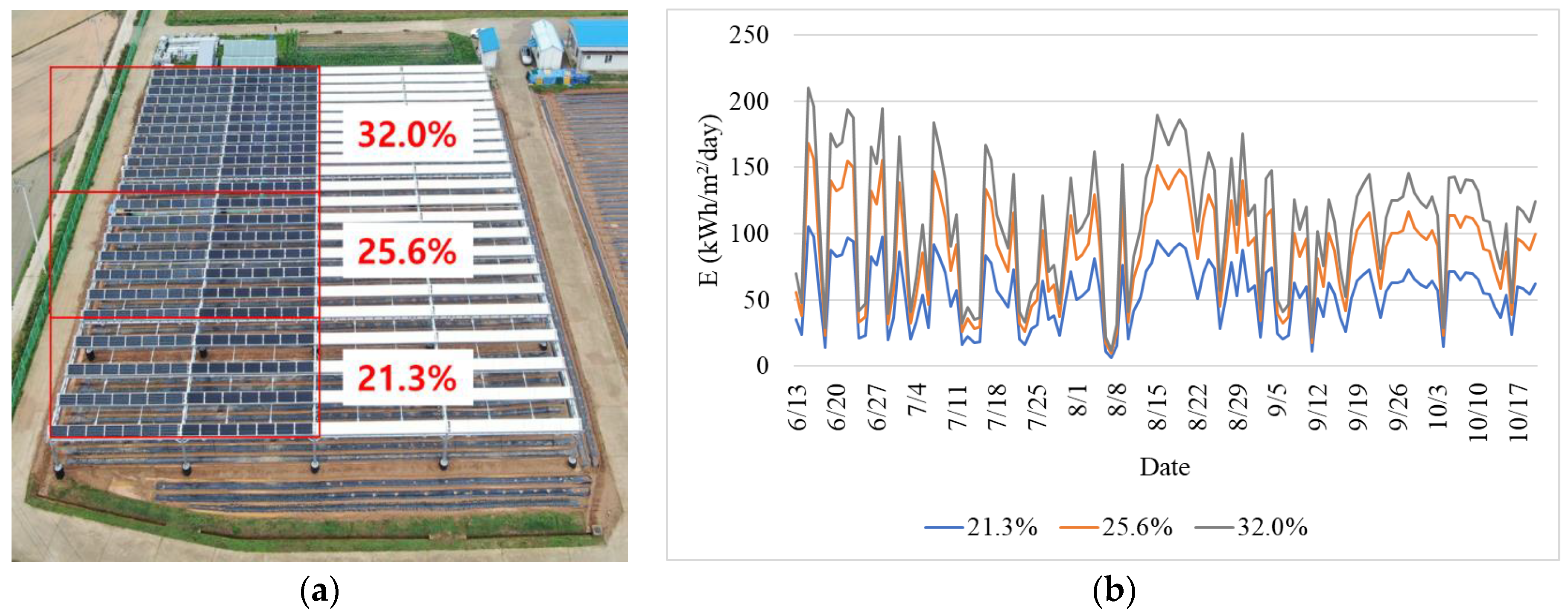
Figure 1. Subject APV system: (a) APV structure; (b) Electricity generation by the APV system. APV: Agrophotovoltaic [7].
Energies 15 06512 g001
Figure 2. The estimated amount of electricity for a 98.8 kW PV power plant.
Energies 15 06512 g002
Table 1. Construction costs of an APV system (edited from Kim et al. [4]).
Data Type21.3%25.6%32%
Total construction cost (USD)17,370.7227,793.1434,741.43
Solar module cost (USD)4961.257938.009922.50
Structure cost (USD)8211.8113,138.9016,423.63
Electric distribution system cost (USD)3911.236257.977822.46
Other costs (USD) 1286.42458.27572.84
Number of PV modules per unit area (units/m2)0.0620.0660.089
Unit construction cost (USD/m2)15.3216.3422.06
1 The costs include the building permit fee and the fee for linkage to the existing electric distribution system.
Table 2. Observed climatic data [7].
MonthSolar Radiation (MJ/m2)Surface Temperature High (°C) 1Surface Temperature Low (°C) 2Precipitation (mm)Humidity (%)Wind Speed (m/s)
June3.7029.4019.4312.7276.932.01
July2.7727.7120.9214.8084.671.94
August3.6234.0524.2517.8373.362.45
September3.0327.7416.747.1774.111.67
October3.2724.688.730.3056.941.67
1 The highest air temperature; 2 the lowest air temperature.
Table 3. Harvested grain yields (Mg/ha) of all five crops grown in four different degrees of shade [4].
Crop TypeShading Ratios (%)
021.325.632
Sesame (Sesamum indicum)0.960.89 (−7%) 10.83 (−14%) 10.45 (−53%) 1
Mung bean (Vigna radiata)1.951.54 (−21%) 11.1 (−44%) 11.09 (−44%) 1
Red bean (Vigna angularis)2.351.75 (−26%) 11.52 (−35%) 11.47 (−37%) 1
Corn (Zea mays)8.098.56 (+6%) 16.4 (−21%) 15.63 (−30%) 1
Soybean (Glycine max)3.643.15 (−13%) 12.88 (−21%) 12.54 (−30%) 1
1 Numbers in parentheses indicate the loss (−) or gain (+) of the yield, compared to the yield without shading.
Table 4. Declination and solar radiation data.
MonthObserved ValuesEstimated Values
δ I δ I
June23.103.7023.353.71
July21.202.7720.933.66
August13.503.6212.973.44
September2.203.031.593.02
October−9.603.27−8.252.57
Table 5. The measured amount of electricity quantity and the estimated amount of electricity.
CategoryShading RatioMonth
JuneJulyAugustSeptemberOctober
Measured Electricity (E, kWh/m2/day)21.3 10.060.040.050.050.05
25.6 20.060.040.060.050.05
32.0 30.080.060.080.070.07
Estimated Electricity (E, kWh/m2/day)21.3 10.050.040.060.050.05
25.6 20.050.040.060.050.06
32.0 30.070.050.080.070.08
1 The size of the PV module ( A p v ) is 1134 m2; 2 The size of PV module ( A p v ) is 1701 m2; 3 The size of the PV module ( A p v ) is 1575 m2.
Table 6. The estimated grain yields (Mg/ha) of all five crops.
Crop TypeShading Ratios (%)
021.325.632
Sesame (Sesamum indicum)0.960.89 (−14%) 10.80 (−17%) 10.76 (−21%) 1
Mung bean (Vigna radiata)1.851.52 (−18%) 11.45 (−21%) 11.36 (−27%) 1
Red bean (Vigna angularis)2.061.69 (−18%) 11.61 (−22%) 11.50 (−27%) 1
Corn (Zea mays)8.096.33 (−22%) 15.98 (−26%) 15.47 (−32%) 1
Soybean (Glycine max)3.813.05 (−20%) 12.90 (−24%) 12.67 (−30%) 1
1 The numbers in parentheses indicate loss (−) or increase (+) in the yield compared to the yield without shading.
Table 7. Observed climate data.
YearSolar Radiation (MJ/m2)Surface Temperature High (°C) 1Surface Temperature Low (°C) 2Precipitation (mm)Humidity (%)Wind Speed (m/s)
201710.0527.6618.404.2779.502.02
20189.5927.8018.467.2376.002.34
201912.2127.1618.507.1277.801.92
202014.9526.7218.248.0578.801.96
202116.7028.1419.066.6979.801.50
1 The highest air temperature; 2 the lowest air temperature.
Table 8. The estimated amount of electricity for a 3 MW PV power plant.
CategoryYear
201820192020
Measured Electricity (E, kWh/day) 112,167.9112,034.9311,519.06
Estimated Electricity (E, kWh/day) 110,323.139733.2211,518.84
1 The size of PV module ( A p v ) is 52,000 m2.
Table 9. Estimated grain yields (Mg/ha) of all five crops.
Plant TypeCrop Type
Sesame (Sesamum indicum)Mung Bean (Vigna radiata)Red Bean (Vigna angularis)Corn (Zea mays)Soybean (Glycine max)
98.8 kW PV Power Plant0.69 (−28%) 11.20 (−35%) 11.32 (−36%) 14.65 (−42%) 12.31 (−39%) 1
3 MW PV Power Plant0.58 (−39%) 10.94 (−49%) 11.02 (−50%) 13.30 (−59%) 11.70 (−55%) 1
1 The numbers in parentheses indicate loss (−) or increase (+) in the yield, compared to the yield without shading in Table 6.
Publisher’s Note: MDPI stays neutral with regard to jurisdictional claims in published maps and institutional affiliations.

