CFD Study of High-Speed Train in Crosswinds for Large Yaw Angles with RANS-Based Turbulence Models including GEKO Tuning Approach

Abstract

Crosswind action on a train poses a risk of vehicle overturning or derailment. To assess if new train designs fulfill the safety requirements, computational fluid dynamics is commonly used. This article presents a comprehensive wind flow analysis on an example of a TGV high-speed train. Large yaw angle range is studied with the application of widely used Reynolds-averaged Navier–Stokes (RANS) turbulence models. The predictive performance of popular RANS-based models in that regime has not been reported extensively before. The context of simulations is a study of crosswind stability using methodology presented in norm EN 14067-6:2018. It is shown that for yaw angles up to 45 degrees, aerodynamic forces predicted by all the studied RANS-based models are consistent with experimental data. At larger yaw angles, flow structure becomes complicated, separation lines are no longer defined by geometry, and significant discrepancies between turbulence models appear, with relative differences between models up to 30%. A detailed study was performed to investigate differences between turbulence models for specific angles of 40, 60, and 80 degrees, which correspond to distinctive ranges of moment characteristics. Finally, a successful attempt was made to tune a GEKO turbulence model to fit the experimental data. This allowed us to reduce the maximum relative error in comparison to the experiment in the full yaw angles range down to 12.7%, which is in line with the norm requirements.

1. Introduction

Crosswind action on a train poses a risk of vehicle overturning or derailment. The risk is elevated not only when wind speed is high, but also in such scenarios as a sudden gust of wind while exiting a tunnel, or when running on a bridge or around curves. Recent trends of increasing train speeds and reducing their weight to lower the energy consumption and track wear are also adverse to safety. In recent years, there have been several accidents caused by strong wind, such as the train overturn in Xinjiang in China in 2007 [1], Lenk in Switzerland in 2018 [2], or Walton in Harvey County in 2019 [3] to name a few. The topic of wind effects on rail vehicles remains of researchers’ interest, and dedicated technical standards are being developed and updated.

Establishing the safety criteria is a multidisciplinary topic, as air–train–track interaction needs to be considered [4,5]. However, one of the first steps is determining aerodynamic forces and moments acting on the train. Full-scale experiments are costly, time-consuming, and give little control over the conditions such as wind speed and direction. Despite the difficulties, some research work has been conducted on a full scale [6,7]. Wind tunnel experiments performed in a reduced scale are much more common. In the last decade, a tool that proved to be useful as complementary to the experiment is the computational fluid dynamics (CFD). Computer simulation reduces the number of experiments that need to be carried out, reduces overall design costs, enables decisions in the early stages of the design process, and allows for an analysis of scenarios that cannot be tested in wind tunnels. Even though CFD in railway industry has become widespread, as evidenced by, inter alia, developed norms [8], it involves a number of challenges—obtaining reliable results is strictly dependent on the used simulation methodology. Norms such as EN 14067-6:2018 allow rolling stock assessment based solely on numerical simulations for train speeds up to a maximum of 200 km/h, however, the appropriateness of the CFD approach has to be firstly demonstrated on a benchmark case. The norms themselves are written in a way that simulation requirements are given, but the simulation methodology is not defined. In order to list the most important key points from the point of view of simulation, it is necessary to indicate: the method of preparing the model and numerical mesh, the selected calculation methods, a reliable representation of boundary conditions, and the modeling of turbulence. While each of the elements mentioned above is necessary to obtain reliable results, most discussion is devoted to the selection of an appropriate turbulence model.

In the context of numerical simulation of vehicle aerodynamics, the literature contains mostly publications devoted to car aerodynamics. CFD is commonly used in the design process to analyze the flow around motorcycles [9] and race cars [10,11], as well as civilian ones [12,13]. Over the past twenty years, simulation methodologies have been developed, and individual approaches’ strengths and weaknesses have been identified [14,15,16]. In the case of numerical analyses of the crosswind affecting trains, the literature is more modest, and many questions remain unanswered. Most of the works reproduce an experimental procedure in which the forces and moments acting on a train subjected to air flow are measured. The train is placed in a tunnel and rotated.

However, in contrast to experimental studies, usually yaw angles tested numerically do not exceed 50 degrees. A summary of the most relevant publications on the topic of CFD simulations of trains in crosswind is presented in the Appendix A in

Table A1. Selected relevant numerical studies on train crosswind stability.

Study	Scenario	Geometry	Reynolds Number	Turbulence Models	Yaw Angle Range	Key Features
Paradot et al. [17]	Stationary train, various inlet profiles	TGV Duplex	N/A	RANS	15°–90°	Wide angle range
Diedrichs [28]	Low turbulence, stationary train	ICE 2	1.4 × 106	RANS	Mostly 20°–40°, angles 50° and 60° for one case	Confirmation of RANS applicability for 20°–40° range
Diedrichs [20]	Low turbulence, stationary train	Regional train	0.2 × 106	RANS, DDES	30° and 41.5°	Comparison of RANS and DDES
Diedrichs et al. [32]	Low turbulence, stationary train	ICE 2	4.6 × 106	RANS	30°	High embankments
Catanzaro et al. [38]	Stationary and moving train	ETR500	N/A	RANS	0°–45°	Comparison between still and moving train
Sima et al. [33]	Low turbulence, stationary train	Various high-speed and regional trains	0.5 × 106	RANS	10°–60°	Comparison of CFD predictions for various train shapes
Morden [39]	10% turbulence intensity, stationary train	Class 43 HST	0.125 × 106	RANS, DES, DDES	015°	Extensive study, i.e., influence of ballast height
Khier et al. [40]	Low turbulence, stationary train	Regional train	3.7 × 106	RANS	0°–90°	Wide angle range
Eichinger et al. [21]	Low turbulence, stationary train	Regional train	0.6 × 106	RANS, URANS, DES, DDES	30°	Various computational domains and turbulence models
Liu et al. [41]	Low turbulence, moving train	CRH2	N/A	RANS	23°	Running from a cutting to an embankment
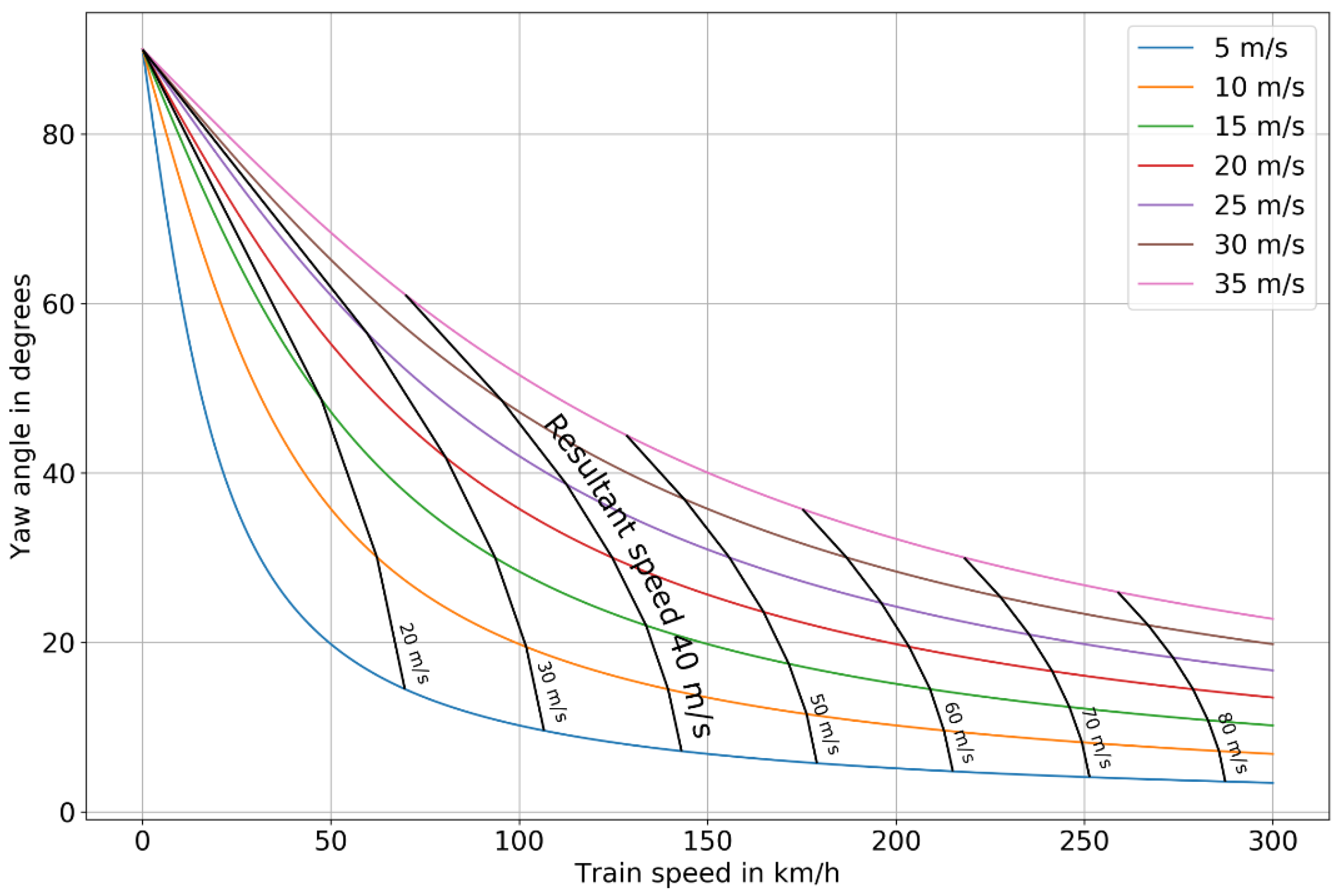
Yao et al. [42]	Low turbulence, moving train	High-speed train	N/A	RANS	25°–70°	Train–bridge system

. In eleven numerical studies devoted to crosswinds, only two investigated the full range of angles, of which only one performed a comparison with experimental data. From the Paradot et al. study [17], one can observe good convergence of the numerical model with experiments for small angles and much larger errors for larger angles. In their research, however, Paradot et al. did not deal with a more detailed study of turbulence models’ accuracy and the ability to predict the phenomena occurring for larger angles. Limited tested angle range is only partially justified by the maximum yaw angles obtained at full train speed. If a strong side wind was blowing at 35 m/s for a high-speed train running at 150 km/h, it would correspond to a yaw angle of 40 degrees. Larger yaw angles are present for regional trains due to their lower running speed. As seen in Figure 1, inflows from angles exceeding 50 degrees are still important as they can occur during acceleration or standstill of the train. Examples of overturning accidents that occurred for a train in standstill or moving below 70 km/h are St. Nicolas in Great Britain in 2015, an Ohio bridge in the USA in 2008, the Chikuhi line in Japan in 1998, or the Kosei line in Japan in 1997 [18].

Figure 2 shows the schematic diagram with velocity vectors. Considering the wind velocity v_w with angle relative to track β and train velocity v_t, the resultant velocity v_r and yaw angle α can be calculated.

The effect of crosswinds is usually presented in the form of a plot of the forces and moments or their coefficients acting on the train as a function of the yaw angle. Figure 3 shows the most important, from the point of view of train overturning, x moment coefficients as a function of yaw angle. Distinct parts can be observed in the characteristic curves. After the initial increase, the moment value reaches the maximum, then decreases or stabilizes at a relatively constant value for the largest angles. As can be seen, the shape of the train body, track configuration, and the turbulence level all affect the characteristic curves. For high values of turbulence, the maximum values of lateral forces occur for larger angles, such as 70 degrees [19]. For larger angles, there are also fundamental differences in simulation methodology planning. Large flow instabilities occur during inflows from angles above 50 degrees. Due to that, the flow around the train is not a trivial scenario from the turbulence modeling standpoint. Regardless, an industry standard is to apply Reynolds-averaged Navier–Stokes (RANS)-based turbulence models. Their computational cost related to more complex unsteady numerical methods, such as scale resolving simulations (SRSs) used in [20,21,22], is orders of magnitude lower. An important open question remains about RANS-based models’ accuracy, especially within the aforementioned range of yaw angles.

The novelty of the article is a comprehensive wind flow analysis at a large yaw angles range of 10–90° for widely used RANS turbulence models. It is a challenging situation from a numerical standpoint, as large separation zones and flow unsteadiness may be expected, which may result in significant differences between RANS-based models. The predictive performance of popular RANS-based models in that regime has not been reported extensively. The most common turbulence models are studied to assess their accuracy and answer the questions:

• How significant are the differences between the RANS-based models in the large yaw angle range?
• What causes these differences?
• Which model fits the experimental data best?

Finally, a methodology for fitting a relatively new generalized k–ω (GEKO) turbulence model to the experimental data is proposed, as an alternative to classical solutions. Successful attempts of tuning the GEKO model were reported in the literature, e.g., in the case of jet flows [23], combustion [24], compressible flows [25], and marine hydrodynamics [26], but to the authors’ knowledge, no attempt of tuning a GEKO model for a train in a crosswind scenario has been reported yet.

2. Materials and Methods

As a test model, a TGV Duplex power car was chosen, as it is one of the benchmark cases described in the norm [8]. There are experimental results available that could be taken as the reference values. Simulations concern a full-scale TGV Duplex power car on a single track with ballast and rail, shown in Figure 4. Standard gauge track of 1435 mm was used. The reference data were based on a single data set measured in the CSTB wind tunnel in Nantes in scale 1:15. The aerodynamic coefficients were measured for the case of zero tilting angle.

The pitching moment coefficient against the leeward rail C_mx,lee is defined according to the norm [8], and is shown with the applied coordinate system in Figure 5. Aerodynamic loads were captured only for the leading train and they were scaled using the reference length d₀ = 3 m and reference area A₀ = 10 m². The air density was set as constant equal to 1.225 kg/m³ and the reference velocity was equal to the inlet wind speed of 32 m/s.

2.1. Geometry and Computational Domain

Aerodynamically significant features on the train side and roof were modeled. The wheels were flattened to prevent point contact with the ground and the pantograph was not modeled, which is a common practice and is allowed by the norm.

Velocity v = 32 m/s was applied at inlet. It corresponds to the wind speed that caused the train overturning at Horei Iwate in Japan in 1994. The resultant Reynolds number was ca. 6.5 × 10⁶. It is commonly assumed that in the range of large Reynolds numbers, force and moment coefficients are independent of the Reynolds number. Technical Specifications for Interoperability (TSI) [27] specify the minimum Reynolds number of 0.25 × 10⁶ to ensure no Reynolds number scaling effects occur. The velocity at the inlet was uniform, to agree with the specifications for wind tunnel measurements.

In the wind tunnel experiments, it was assumed that the boundary layer thickness δ_99% shall not exceed 30% of the vehicle height and that the turbulence level does not exceed 2.5%. Therefore, low-turbulence intensity boundary conditions were applied in the simulation: turbulence intensity at a low value of 2% and turbulent length scale 0.01 m. High turbulence intensity can have a significant impact on the results for large yaw angles, as shown in [19].

All wall surfaces were stationary. No-slip condition was applied to the walls, which means the velocity at the walls was zero. Side and top surfaces were given symmetry boundary conditions, i.e., zero normal velocity v_n and zero gradient of all quantities ∂φ/∂n = 0. Zero gauge static pressure p was prescribed at the outlet.

Appropriate domain size was set to not interfere with the flow around the vehicle. The domain lengths upstream and downstream were equal to 20H and 33H, respectively, where H is the train height. The blockage ratios, as well as upstream and downstream size of the domain, were defined based on the norm requirements. Exact dimensions are shown in Figure 6 for an exemplary yaw angle of 55 degrees.

2.2. Mesh

A relatively uniform surface mesh was applied to the train body, as shown in Figure 7a. Three box-shaped refinement regions were added in the vicinity of the train to capture regions of high pressure and velocity gradients. Location, shape, and size of refinement regions are not specified in the norm. It was firstly selected based on our experience and literature review. At a later step, regions of large gradients were displayed to confirm the validity of the adopted meshing methodology. The mesh design has been kept for all the studied yaw angles.

Volume mesh consisted of tetrahedral elements with a prism boundary layer, as shown in Figure 7b. The boundary layer mesh consisted of 10 elements. The dimensionless wall distance y⁺ for the first cell layer on the train surface was kept in the range of wall function validity. Other studies [28] have shown that in this simulation scenario the approach with the first cell in the viscous sublayer to represent the near-wall regime does not seem favorable over wall functions.

It was important to consider geometrical features at the meshing stage, as even small features may have a significant impact on the flow structure. One such example was a sharp edge on the roof, which is present in the original geometry. For large yaw angles, it defines the separation point. If this feature was not preserved explicitly at the meshing stage, flow would remain attached to the roof. Figure 8 shows a comparison of flow structures on the train roof in the middle of the leading train, for a yaw angle of 80 degrees. With a correctly preserved sharp edge on the roof, a clear separation line was visible. Without the sharp edge, flow remained attached to the roof. As a result, there was a relative difference of 10% in rolling moment coefficient between these two cases.

Grid sensitivity was assessed by changing the tetrahedral cell size in the region of high pressure and velocity gradients, shown in Figure 9. Characteristic cell size was changed by a factor of 1.5. The grid independence test has been performed for two yaw angles, 20 degrees and 75 degrees.

The results showed good agreement in terms of flowfield and moment coefficients, as shown in

Table 1. Grid sensitivity results. C_mx,lee for various meshes.

Yaw Angle in Degrees	Coarse	Medium	Fine
20	2.331 (+1.8%)	2.290 (+0.0%)	2.289
75	4.690 (+2.7%)	4.575 (+0.2%)	4.567

. The relative differences of rolling moment coefficient for the small angle of 20 degrees did not exceed 2% for all the studied meshes. In the case of a large yaw angle, 75 degrees, the differences did not exceed 3%. It was therefore assumed that further computations could be continued on the 46 mln mesh.

2.3. Solver

All presented simulations were performed in ANSYS Fluent software version 2021 R2, in which incompressible Reynolds-averaged Navier–Stokes (RANS) equations were solved using a finite-volume method. Using the Einstein summation convention, the continuity equation takes the form of:

$$\frac{\partial {\overline{v}}_i}{\partial x_i}=0$$

(1)

and the momentum conservation equation can be written as:

$$\rho \left(\frac{\partial {\overline{v}}_i}{\partial t}+{\overline{v}}_j\frac{\partial {\overline{v}}_i}{\partial {\overline{v}}_j}\right)=-\frac{\partial \overline{p}}{\partial x_i}+\frac{\partial }{\partial x_j}\left[\mu \left(\frac{\partial {\overline{v}}_i}{\partial x_j}+\frac{\partial {\overline{v}}_j}{\partial x_i}\right)-\rho \overline{v{\prime }_{i}v{\prime }_j}\right]$$

(2)

where v_i represents the i-th component of velocity at a point x_i in space, ρ is the fluid density, p represents the static pressure, μ is the dynamic viscosity, δ_ij is the Kronecker delta, bars denote averaged values, and apostrophes represent fluctuating values. In steady-state RANS, the transient term in Equation (2) vanishes. Due to the Reynolds stress tensor $-\rho \overline{v{\prime }_{i}v{\prime }_j}$, the closure problem arises, and additional equations are needed. They are supplemented by turbulence models, which can be roughly categorized in two basic groups: models that solve transport equations for Reynolds stress tensor components and models that follow the Boussinesq hypothesis and introduce turbulent viscosity. The turbulence models selected for this work belong to the latter group. It is assumed that the Reynolds stress tensor is proportional to the mean strain rate tensor:

$$-\rho \overline{v{\prime }_{i}v{\prime }_j}={\mu }_t\left(\frac{\partial {\overline{v}}_i}{\partial x_j}+\frac{\partial {\overline{v}}_j}{\partial x_i}\right)$$

(3)

where μ_t is the turbulent viscosity.

The following models were used: Spalart–Allmaras, realizable k–ε with standard wall function and a production limiter, and k–ω SST. These models are commonly used in external aerodynamics. Additionally, k–ω GEKO with various tunable coefficients settings was tested. The complete list of studied turbulence models can be found in Section 3.4.

The aforementioned RANS models are widely used in external aerodynamics despite a number of inherent limitations. It is known that they are mostly unable to correctly represent the behavior of the detachment regions and transient effects. At the same time, these models make it possible to predict the behavior of the boundary layer quickly and accurately. The accuracy of RANS models depends on many factors, one of the most significant being the shape of a streamlined object. In the literature, one can find many publications devoted to the accuracy of classical turbulence models, such as: for the body of a sedan-type passenger car, Zhang et al. [29] obtained values of aerodynamic coefficients in the error range of 1.3–13.8% compared to the experiment. The most accurate results were obtained with the k–ε model. In the study of car aerodynamics conducted by Kurec et al. [30], discrepancies in the results from different turbulence models depending on the rear wing’s angle were observed. In a paper by Ashton et al. [31], based on Ahmed and DrivAer body simulations, it was summarized that RANS models are sensitive to car body types and it is difficult to determine guidelines for choosing a particular turbulence model in the general case. It was estimated that 5% is the limit of the models’ accuracy—more costly hybrid or LES models are needed to achieve higher accuracies. Thus, in the classical approach, one of the important elements of planning a numerical experiment is the selection of a turbulence model. Even with reference data in the form of experimental results, calibration is carried out in a discrete way: we can choose specific turbulence models, possibly modifying some used submodels. A completely different approach was proposed in [16] by Menter, Lechner, and Matyushenko, who presented the GEKO model—destined to become a new paradigm in turbulence modeling.

The GEKO turbulence model provides six free parameters that can be calibrated based on experimental data. A list of tunable parameters together with their roles is shown in

Table 2. The function and recommended range of GEKO free coefficients.

Parameter	Function	Recommended Range	Default Value
CSEP	Separation prediction	0.7–2.5	1.75
CNW	Wall shear stress and wall heat transfer in equilibrium flows	−2.0–2.0	0.5
CMIX	Mixing strength of free shear flows	0.5–1.0	$0{.35\mathrm{sgn}(C}_{\mathit{SEP}}-1)·$ $\sqrt{{|C}_{\mathit{SEP}}-1|}$
CJET	Jet spreading rate	0.0–1.0	0.9
CCORNER	Secondary flows in corners	0.0–1.5	1.0
CCURV	Curvature correction	0.0–1.5	1.0

. With default settings (C_SEP = 1.75, C_NW = 0.5, C_JET = 0.9, and C_MIX calculated from a correlation), GEKO is supposed to mimic the performance of the k–ω SST model. In addition to the seamless adjustment of parameters themselves, even locally, what sets the GEKO model apart from other models is its attempt to link parameters to specific flow phenomena.

A pressure-based solver, implicit formulation, and Green–Gauss node-based method for the calculation of gradients were used for all the studied cases. Simulations were performed in steady-state and the coupled pseudo-transient scheme was applied for pressure–velocity coupling. Second-order spatial discretization was set for pressure and momentum. For comparative purposes, for yaw angles of 60° and 80°, transient simulations were also performed with Δt = 70 ms.

Forces and moments acting on the train were monitored throughout the iterative calculation process. The convergence criteria were stabilized residuals and stabilized forces and moment monitors. If oscillations were present, then iterative calculations were run until 5–10 periods of stable oscillations were captured. The iteration errors were an order of magnitude lower than the discretization errors.

Unless noted as instantaneous values, presented data concern averaged data from stable oscillation cycles. Nondimensional velocity, which is reported in contour maps and vector fields, is the local velocity divided by the inlet velocity of 32 m/s.

2.4. Computational Resources

Calculations were performed on the high-performance computing infrastructure provided by the National Centre for Nuclear Research (Poland). The average calculation time of a single case on 200 physical cores (i.e., 5 computational nodes as specified in

Table 3. Single computational node short specification.

Component	Specification
CPU	2 × Intel(R) Xeon(R) Gold 6248 2 × 20 = 40 physical cores @2.5/3.9 GHz (without Hyper-Threading)
RAM	192 GB
HDD	480 GB SSD
Interconnect	Infiniband

) was 130 min. The calculation time was measured as the difference between job start and finish, so it includes reading mesh and saving case and data files.

3. Results

3.1. Global Parameters

The main objective of the crosswind analysis is to estimate the forces that may overturn the train. From this point of view, the most important is the C_mx,lee value, which determines the moment coefficient that turns the train over. It is calculated relative to a reference point defined by the top of the rail on the leeward side.

The reproducibility requirements for CFD stated in the EN14067-6:2018 are similar to those of a wind tunnel. Maximum relative differences of the rolling moment coefficient between the experiment and simulation should not exceed 15%. Simultaneously, the mean value of relative error should be below 10%:

$$\max \left(\left|\frac{C_{\mathit{mx,lee,test}}-C_{\mathit{mx,lee,bmk}}}{C_{\mathit{mx,lee,bmk}}}\right|\right) {<\epsilon }_{\mathit{max}},$$

(4)

$$\mathrm{mean}\left(\left|\frac{C_{\mathit{mx,lee,test}}-C_{\mathit{mx,lee,bmk}}}{C_{\mathit{mx,lee,bmk}}}\right|\right){<\epsilon }_{\mathit{mean}}.$$

(5)

Figure 10a shows the characteristics of the C_mx,lee coefficient as a function of the flow direction for the different turbulence models compared with the experimental data from [8]. As can be seen, for small inflow angles up to 45 degrees, an excellent agreement of results between turbulence models was obtained with max. relative error of 3.5%. In turn, there are substantial differences for higher ranges depending on the chosen turbulence model. In Figure 10b, the obtained errors are presented with the indication of the 15% threshold of relative error, which is imposed by the norm [8]. As can be seen, the results from none of the turbulence models would meet the requirements of the norm.

Interestingly, we can distinguish two areas in which we observe different trends of models. In the region of characteristic inflection (50–65 degrees), good convergence was obtained for the k–ε model with k–ω and S–A outliers. On the other hand, we observe the opposite trend for the range when the characteristics flatten out. To find the causes of the differences between the indicated ranges, a detailed flow analysis for angles 40, 60, and 80 degrees was performed. In [28], similar agreement of RANS results and experiments was reported for low yaw angles. In [28,32,33], various RANS turbulence models were studied and differences between models were of the same order of magnitude as in this paper for low yaw angles below 40 degrees.

3.2. Analysis of Flow Structures

Figure 11 compares pathlines released from the train surface for the analyzed angles. The observed flow structures are in line with reported studies of flow past yawed slender bodies [34]. At lower yaw angles, up to 40 degrees, the flow is attached to the rooftop surface. At incidences between 40 and 60 there is a quasi-steady regime. At incidences above about 60, the flow is unsteady, being qualitatively similar to the well-known flow past a cylinder at 90 to the stream, with vortex shedding phenomena.

For the angles of 60 and 80 degrees, it was verified that the steady-state pseudo-transient results are in line with averaged transient results, as shown in

Table 4. Comparison of results obtained with RANS pseudo-transient and URANS approaches.

Yaw Angle in Degrees	Cmx,lee RANS Pseudo-Transient	Cmx,lee URANS with Δt = 70 ms
60	7.76	8.04 (+3.7%)
80	5.07	4.99 (+1.6%)

. For yaw angles above 60, oscillations became more pronounced. This may be observed on root mean squared error (RMSE) of pressure coefficient C_p contour maps shown in Figure 12. RMSE was calculated using the following formula:

$$C_{p \mathrm{RMSE}}=\sqrt{\frac{\sum {\left(C_p-C_{p \mathrm{avg}}\right)}^2}{n}}$$

(6)

where C_p is the pressure coefficient value in the current iteration, n is the number of iterations, and C_{p avg} is the averaged value of pressure coefficient from five oscillation cycles.

Figure 13 compares vortex core locations and separation lines for angles of 40, 60, and 80 degrees. These flow structures were calculated in ANSYS EnSight 2022R1, with the use of algorithms described in [35,36,37]. For the yaw angle of 40 degrees, the flow was attached to the roof of the train, with a clear separation line at the leeward edge. At 60 degrees, a separation region started to form in the middle of the leading train. At 80 degrees, detachment occurred on the roof. Interestingly, it was characterized by a spatial structure. It was demonstrated that at larger yaw angles separation points are no longer well-defined and discrepancies between turbulence models can be expected. At the same time, as studied in [28], the lee-rail moment obtains its greater contribution from the upper leeward part of the train body. Differences found near the ground are contributing less to the lee-rail moment, as a consequence of a relatively small leverage. Observed structures are consistent with a description already reported in literature for the case of high-speed trains in crosswind [28].

3.3. Comparison of Flow Structures between Turbulence Models

In the following paragraphs, differences in flow structures captured by various turbulence models are discussed for low, medium, and high yaw angles of 40, 60, and 80 degrees. GEKO with C_SEP = 2.5 was added to the previously reported set of turbulence models. This was due to the fact that it provided the best performance in the whole yaw angle range. Additional data on this topic are presented in Section 3.4.

The following images show data captured on a plane perpendicular to the train, located in its middle length. Looking at the velocity distributions in Figure 14, one can see that for the angle of 40 degrees, the predicted flow structure was similar for all RANS models. However, for the angles of 60 and 80 degrees, significant differences were observed.

As illustrated in Figure 14a, when it comes to low yaw angles, the results were similar in terms of qualitative comparison regardless of turbulence model used, with just minor quantitative deviations. It is clearly visible that the minimal deviation of C_mx,lee which is reported in Figure 10 was not just a coincidence.

For a higher yaw angle, i.e., 60 degrees, turbulence model choice became a key factor. What can be seen in Figure 14b is the qualitative difference between the models’ response, especially when it comes to Spalart–Allmaras. In Figure 10, Spallart–Allmaras was also the outlier. The best fit to the experimental data was achieved for realizable k–ε and then GEKO, accordingly. Comparison between all other models apart of Spalart–Allmaras brings some similarities. Each pair combined out of these three models shares certain flow features. In the area at the leeward side of the train, above the roof, resemblances of flowfields predicted by realizable k–ε and GEKO can be observed. Closer to ground level, similarities in the flowfield predicted by GEKO and k–ω SST are seen. As both realizable k–ε and GEKO fit the experimental results best, one can come to the conclusion that proper recreation of the flow above the train roof and in the passage of detached flow on the leeward side may have a crucial role when assessing C_mx,lee.

For yaw angles as high as 80 degrees, the situation became even more ambiguous, as shown in Figure 14c. One should take into account that Figure 14 presents a cross-section of highly three-dimensional flow structures. The location of boundary layer detachment lines on the roof had a significant impact on flow development on the leeward side.

Failure to predict separation seemed to be a reason for realizable k–ε failure, as shown in Figure 15.

3.4. Calibration of GEKO Turbulence Model to Fit the Experimental Data

GEKO turbulence models provide six tunable parameters. It was verified by the authors in a series of preliminary simulations that in the case of the studied scenario of a train in crosswind, only the C_SEP parameter had a significant impact on the observed rolling moment coefficient. This was expected, as C_SEP is a parameter designed to optimize flow separation from smooth surfaces.

A summary of the obtained moment coefficients is presented in

Table 5. Mean square root error, as well as mean and maximum values of relative error, of the rolling moment coefficient for various turbulence models.

Turbulence Model	MSE of Cmx,lee	Max. Absolute Value of Relative Error of Cmx,lee	Mean Absolute Value of Relative Error of Cmx,lee
GEKO, CSEP = 3.00	0.16	12.3	5.6
GEKO, CSEP = 2.50	0.17	12.7	6.1
k–ω SST	0.23	17.1	6.1
GEKO, CSEP = 2.10	0.26	14.9	7.6
Realizable k–ε	0.34	19.2	8.3
GEKO, CSEP = 1.75 (default)	0.38	18.9	9.3
GEKO, CSEP = 1.40	0.38	16.7	9.4
GEKO, CSEP = 1.00	0.54	24.9	10.5
Spalart–Allmaras	0.70	34.3	7.9

. To present data in a concise manner, mean square error (MSE) was calculated for each case, together with the maximum and mean absolute value of relative error with respect to the experiment.

Turbulence models are sorted starting from the lowest MSE. The best match with the experimental data was obtained for GEKO with C_SEP equal to 3.0. Simulations performed with these turbulence models would pass the requirements of the norm in the whole yaw angle range. Promising results were obtained with k–ω SST, but in this case the maximum value of relative error exceeded 15%. Interestingly, GEKO with default settings had a worse performance than k–ω SST which it was supposed to mimic.

It has been shown in a number of studies, e.g., [28], that relative errors of lift and side forces are usually larger than those of the rolling moment. The agreement for the two orthogonal loads is worse and errors compensate. To check if this was the case, lift and side forces errors were also computed. Results are presented in

Table A2. Mean square root error, as well as mean and maximum values of relative error, of the lateral force for various turbulence models.

Turbulence Model	MSE of Cy	Max. Relative Error of Cy	Mean Relative Error of Cy
GEKO, CSEP = 2.50	0.32	11.6	6.5
GEKO, CSEP = 3.00	0.38	13.4	7.4
GEKO, CSEP = 2.10	0.52	15.1	8.2
k–ω SST	0.57	20.3	7.3
GEKO, CSEP = 1.75	0.75	20.2	10.4
GEKO, CSEP = 1.40	0.76	18.8	10.5
Realizable k–ε	0.84	23.3	9.5
GEKO, CSEP = 1.00	1.02	24.9	11.5
S–A	1.34	35.5	9.9

and

Table A3. Mean square root error, as well as mean and maximum values of relative error, of the vertical force for various turbulence models.

Turbulence Model	MSE of Cz	Max. Relative Error of Cz	Mean Relative Error of Cz
GEKO, CSEP = 3.00	0.18	25.0	8.4
GEKO, CSEP = 2.50	0.31	26.6	11.0
GEKO, CSEP = 2.10	0.35	23.6	10.6
GEKO, CSEP = 1.75	0.72	29.9	15.4
k–ω SST	0.97	47.0	19.9
GEKO, CSEP = 1.40	1.26	40.0	21.1
S–A	1.42	42.8	20.3
Realizable k–ε	1.81	52.7	26.3
GEKO, CSEP = 1.00	2.88	56.7	33.1

in the Appendix A. In this study, relative errors of lift and side forces were also larger than those of the moment coefficient. However, as it turns out, turbulence models which best matched C_mx,lee data also had the best performance for orthogonal loads.

In Figure 16, relative errors of rolling moment coefficient for different C_SEP parameter values are presented. C_SEP 1.0 and 3.0 are the extreme values used in this study and C_SEP = 1.75 is the default value. It can be observed that low C_SEP values started to noticeably affect the solution starting from the yaw angle of 30 degrees.

The relationship between relative errors and C_SEP value is presented in Figure 17. A gradual reduction in errors can be observed as C_SEP increases. There is a marginal difference between C_SEP 2.5 and 3.0. All variants from C_SEP 2.1 to 3.0 would pass the benchmark requirements with respect to relative error values.

The influence of C_SEP on the flowfield is shown in Figure 18, which presents a velocity field in the cross-section in the middle of the leading train. Yaw angle of 60 degrees was selected for this comparison, as largest differences between models could be observed there. Changing C_SEP did not affect the separation point on the roof. Instead, the size of the vortex in the train wake and its distance from the train body was increasing monotonically with increasing C_SEP. This affected both velocity values and the suction pressure at the leeward side of the train. With increasing C_SEP, the pressure difference between windward and leeward sides of the train decreases and decreased rolling moment coefficient was obtained.

Pathlines presented in Figure 19 and Figure 20 confirm the main difference between various GEKO C_SEP settings, which was the size of the main vortex which started at the front face of the train. Additionally, the main vortex was extended further from the train for increasing C_SEP.

Calibrating the GEKO model allowed us to obtain aerodynamic forces and moments which were better matched to the experimental values than classically used RANS-based turbulence models, and allowed us to meet the requirements of the norm.

For the studied case of a high-speed train, the best results were obtained for high values of C_SEP. It can be expected that for significantly different geometries, such as regional trains, there would be a need to repeat the calibration process and find optimal C_SEP values.

4. Conclusions

Simulations of a train in crosswind for a wide angle range were presented. The final conclusions of study are as follows:

• The predictive performance of RANS models was assessed, as they are most frequently used in this scenario due to their small computational cost. For angles up to 40 degrees, no significant differences were captured between models, both qualitatively and quantitatively. For higher yaw angles, significant differences between turbulence models appeared and none of the classically used turbulence models would meet the requirements of the norm over the entire range of yaw angles.
• Flowfield was analyzed in detail and separation prediction on the upper leeward edge was identified as having the greatest impact on the results.
• A successful calibration of the tunable GEKO turbulence model was presented. The C_SEP parameter proved to have a significant and consistent impact on the results. Increasing C_SEP values to 2.1 and above reduced the relative errors to levels acceptable by the norm over the entire range of examined yaw angles. The main difference between various C_SEP values was the size of the main vortex which was created at the leading edge of the train. For yaw angles from 30 to 65, where this vortex is significant, increasing C_SEP increased its size. This lowered the rolling moment coefficient and provided a better match with the experimental data.
• An open question and limitation of the study is transferring presented methodology to other train types. The methodology can be repeated in the future for other train geometries, both for high high-speed trains and regional trains, but requires additional validation. In addition, it should be noted that GEKO calibration requires the experimental data, which could be the main limitation in many studies.

References

1. Four Die after Train Derails in China. Available online: http://www.chinadaily.com.cn/china/2007-02/28/content_816203.htm (accessed on 30 June 2022).
2. Storm Burglind Causes Havoc in Switzerland, Derails Train. Available online: https://www.swissinfo.ch/eng/wind-up_switzerland-battered-by-hurricane-speed-winds/43795876 (accessed on 30 June 2022).
3. August 18th 2019 Train Derailment. Available online: https://www.weather.gov/ict/event_2019trainderail (accessed on 30 June 2022).
4. Zhai, W.; Yang, J.; Li, Z.; Han, H. Dynamics of high-speed train in crosswinds based on an air-train-track interaction model. Wind Struct. 2015, 20, 143–168. [Google Scholar] [CrossRef]
5. Xu, Y.L.; Ding, Q.S. Interaction of railway vehicles with track in crosswinds. J. Fluids Struct. 2006, 22, 295–314. [Google Scholar] [CrossRef]
6. Gallagher, M.; Morden, J.; Baker, C.; Soper, D.; Quinn, A.; Hemida, H.; Sterling, M. Trains in crosswinds—Comparison of full-scale on-train measurements, physical model tests and CFD calculations. J. Wind Eng. Ind. Aerodyn. 2018, 175, 428–444. [Google Scholar] [CrossRef]
7. Kikuchi, K.; Suzuki, M. Study of aerodynamic coefficients used to estimate critical wind speed for vehicle overturning. J. Wind Eng. Ind. Aerodyn. 2015, 147, 1–17. [Google Scholar] [CrossRef]
8. EN 14067-6; Railway Applications—Aerodynamics—Part 6: Requirements and Test Procedures for Cross Wind Assessment. CEN: Brussels, Belgium, 2018.
9. Wiński, K.; Piechna, A. Comprehensive CFD Aerodynamic Simulation of a Sport Motorcycle. Energies 2022, 15, 5920. [Google Scholar] [CrossRef]
10. Szudarek, M.; Piechna, J. CFD Analysis of the Influence of the Front Wing Setup on a Time Attack Sports Car’s Aerodynamics. Energies 2021, 14, 7907. [Google Scholar] [CrossRef]
11. Piechna, J.R.; Kurec, K.; Broniszewski, J.; Remer, M.; Piechna, A.; Kamieniecki, K.; Bibik, P. Influence of the car movable aerodynamic elements on fast road car cornering. Energies 2022, 15, 689. [Google Scholar] [CrossRef]
12. Jakirlic, S.; Kutej, L.; Basara, B.; Tropea, C. Computational study of the aerodynamics of a realistic car model by means of RANS and hybrid RANS/LES approaches. SAE Int. J. Passeng. Cars-Mech. Syst. 2014, 7, 559–574. [Google Scholar] [CrossRef]
13. Szudarek, M.; Kamieniecki, K.; Tudruj, S.; Piechna, J. Towards Balanced Aerodynamic Axle Loading of a Car with Covered Wheels—Inflatable Splitter. Energies 2022, 15, 5543. [Google Scholar] [CrossRef]
14. Menter, F.R.; Kuntz, M.; Langtry, R. Ten years of industrial experience with the SST turbulence model. Turbul. Heat Mass Transf. 2003, 4, 625–632. [Google Scholar]
15. Menter, F.; Hüppe, A.; Matyushenko, A.; Kolmogorov, D. An overview of hybrid RANS–LES models developed for industrial CFD. Appl. Sci. 2021, 11, 2459. [Google Scholar] [CrossRef]
16. Menter, F.R.; Lechner, R.; Matyushenko, A. Best Practice: Generalized k-ω Two-Equation Turbulence Model in ANSYS CFD (GEKO); Technical Report; ANSYS: Canonsburg, PA, USA, 2019. [Google Scholar]
17. Paradot, N.; Angel, B.; Gautier, P.E.; Cléon, L.M. Numerical Simulation and Experimental Investigation of the Side Loading on a High Speed Train. Eng. Turbul. Model. Exp. 2005, 6, 657–666. [Google Scholar] [CrossRef]
18. Kocoń, A. Modelling the Phenomenon of Freight Trains Rollover under Crosswind Action. Ph.D. Thesis, Politechnika Krakowska, Kraków, Poland, 2020. [Google Scholar]
19. Bocciolone, M.; Cheli, F.; Corradi, R.; Muggiasca, S.; Tomasini, G. Crosswind action on rail vehicles: Wind tunnel experimental analyses. J. Wind Eng. Ind. Aerodyn. 2008, 96, 584–610. [Google Scholar] [CrossRef]
20. Diedrichs, B. Aerodynamic crosswind stability of a regional train model. Proc. Inst. Mech. Eng. Part F J. Rail Rapid Transit 2010, 224, 580–591. [Google Scholar] [CrossRef]
21. Eichinger, S.; Sima, M.; Thiele, F. Numerical simulation of a regional train in cross-wind. Proc. Inst. Mech. Eng. Part F J. Rail Rapid Transit 2015, 229, 625–634. [Google Scholar] [CrossRef]
22. Maleki, S.; Burton, D.; Thompson, M.C. Assessment of various turbulence models (ELES, SAS, URANS and RANS) for predicting the aerodynamics of freight train container wagons. J. Wind Eng. Ind. Aerodyn. 2017, 170, 68–80. [Google Scholar] [CrossRef]
23. Li, Z.; Liu, Y.; Zhou, W.; Wen, X.; Liu, Y. Thermal pollution level reduction by sweeping jet-based enhanced heat dissipation: A numerical study with calibrated Generalized k-ω (GEKO) model. Appl. Therm. Eng. 2022, 204, 117990. [Google Scholar] [CrossRef]
24. Strokach, E.; Zhukov, V.; Borovik, I.; Sternin, A.; Haidn, O.J. Simulation of a GOx-GCH4 Rocket Combustor and the Effect of the GEKO Turbulence Model Coefficients. Aerospace 2021, 8, 341. [Google Scholar] [CrossRef]
25. Jung, Y.K.; Chang, K.; Bae, J.H. Uncertainty Quantification of GEKO Model Coefficients on Compressible Flows. Int. J. Aerosp. Eng. 2021, 2021, 9998449. [Google Scholar] [CrossRef]
26. Sharkey, P.S.; Menter, F.R. A numerical investigation of the turbulent flow around a scale model JBC hull using the Generalized k-omega (GEKO) turbulence model. In Proceedings of the 11th International Workshop on Ship and Marine Hydrodynamics (IWSH2019), Hamburg, Germany, 22–25 September 2019. [Google Scholar]
27. TSI. Relating to the ‘Rolling Stock’ Sub-System of the Trans-European High-Speed Rail System, 2008/232/CE. Off. J. Eur. Union 2008. [Google Scholar]
28. Diedrichs, B. Aerodynamic Calculations of Crosswind Stability of a High-Speed Train Using Control Volumes of Arbitrary Polyhedral Shape. In Proceedings of the BBAA VI International Colloquium on: Bluff Bodies Aerodynamics Applications, Milano, Italy, 20–24 July 2008; Volumn 20. Available online: http://bbaa6.mecc.polimi.it/uploads/treni/cwt1.pdf (accessed on 1 June 2022).
29. Zhang, C.; Bounds, C.P.; Foster, L.; Uddin, M. Turbulence Modeling Effects on the CFD Predictions of Flow over a Detailed Full-Scale Sedan Vehicle. Fluids 2019, 4, 148. [Google Scholar] [CrossRef]
30. Kurec, K.; Remer, M.; Mayer, T.; Tudruj, S.; Piechna, J. Flow control for a car-mounted rear wing. Int. J. Mech. Sci. 2018, 152, 384–399. [Google Scholar] [CrossRef]
31. Ashton, N.; West, A.; Lardeau, S.; Revell, A. Assessment of RANS and DES methods for realistic automotive models. Comput. Fluids 2016, 128, 1–15. [Google Scholar] [CrossRef]
32. Diedrichs, B.; Sima, M.; Orellano, A.; Tengstrand, H. Crosswind stability of a high-speed train on a high embankment. Proc. Inst. Mech. Eng. Part F J. Rail Rapid Transit 2007, 221, 205–225. [Google Scholar] [CrossRef]
33. Sima, M.; Eichinger, S.; Blanco, A.; Ali, I. Computational fluid dynamics simulation of rail vehicles in crosswind: Application in norms and standards. Proc. Inst. Mech. Eng. Part F J. Rail Rapid Transit 2015, 229, 635–643. [Google Scholar] [CrossRef]
34. Mair, W.A.; Stewart, A.J. The flow past yawed slender bodies, with and without ground effects. J. Wind Eng. Ind. Aerodyn. 1985, 18, 301–328. [Google Scholar] [CrossRef]
35. Sujudi, D.; Haimes, R. Identification of swirling flow in 3-D vector fields. In Proceedings of the 12th Computational Fluid Dynamics Conference, San Diego, CA, USA, 19–22 June 1995; p. 1715. [Google Scholar] [CrossRef]
36. Kenwright, D.; Haimes, R. Vortex identification-applications in aerodynamics: A case study. In Proceedings of the Visualization’97, Phoenix, AZ, USA, 21 October 1997; pp. 413–416. [Google Scholar] [CrossRef]
37. Kenwright, D. Automatic detection of open and closed separation and attachment lines. In Proceedings of the Visualization’98, Research Triangle Park, NC, USA, 18–23 October 1998; pp. 151–158. [Google Scholar] [CrossRef]
38. Catanzaro, C.; Cheli, F.; Rocchi, D.; Schito, P.; Tomasini, G. High-speed train crosswind analysis: CFD study and validation with wind-tunnel tests. Lect. Notes Appl. Comput. Mech. 2016, 79, 99–112. [Google Scholar] [CrossRef]
39. Morden, J.A. A Numerical Investigation of the Effects of Crosswinds Upon the Aerodynamic Characteristics of a High-Speed Passenger Train and Its Slipstream. Ph.D. Thesis, University of Birmingham, Birmingham, UK, 2016. [Google Scholar]
40. Khier, W.; Breuer, M.; Durst, F. Flow structure around trains under side wind conditions: A numerical study. Comput. Fluids 2000, 29, 179–195. [Google Scholar] [CrossRef]
41. Liu, T.; Chen, Z.; Zhou, X.; Zhang, J. A CFD analysis of the aerodynamics of a highspeed train passing through a windbreak transition under crosswind. Eng. Appl. Comput. Fluid Mech. 2018, 12, 137–151. [Google Scholar] [CrossRef] [Green Version]
42. Yao, Z.; Zhang, N.; Chen, X.; Zhang, C.; Xia, H.; Li, X. The effect of moving train on the aerodynamic performances of train-bridge system with a crosswind. Eng. Appl. Comput. Fluid Mech. 2020, 14, 222–235. [Google Scholar] [CrossRef]
Figure 1. Yaw angles and resultant speeds for wind blowing from the side (β = 90°), for various train and wind speeds.
Energies 15 06549 g001
Figure 2. Schematic diagram for determining the yaw angle.
Energies 15 06549 g002
Figure 3. Cmx moment coefficients in function of yaw angle: (a) Different train bodies and embankments, data from [8]; (b) influence of the turbulence intensity on the moment coefficients, data from [19]; *—in [19], the Cmx for the ETR 480 was calculated using different reference values than used for TGV Duplex and ICE 3 in [8].
Energies 15 06549 g003
Figure 4. Studied geometry of a TGV Duplex power car on a single track with ballast and rail.
Energies 15 06549 g004
Figure 5. Coordinate system applied in the study and moments.
Energies 15 06549 g005
Figure 6. Computational domain: (a) Isometric view; (b) top view, 1—train, 2–4—mesh refinement zones, 5—rest of the domain. Black arrows denote flow direction.
Energies 15 06549 g006
Figure 7. Computational mesh: (a) Surface mesh on the leading train; (b) close-up of inflation layer on the train roof.
Energies 15 06549 g007
Figure 8. Effect of omitting the sharp roof edge at the meshing stage on velocity field. Nondimensional velocity is the local velocity divided by the inlet velocity of 32 m/s.
Energies 15 06549 g008
Figure 9. Cross-sections of computational meshes used in the grid independence study: (a) Coarse mesh, 46 mln elements; (b) medium mesh, 60 mln elements; (c) fine mesh, 107 mln elements.
Energies 15 06549 g009aEnergies 15 06549 g009b
Figure 10. Rolling moment coefficient around the leeward rail in function of yaw angle for the most used RANS-based turbulence models: (a) Moment coefficient; (b) relative error in comparison to experimental values.
Energies 15 06549 g010aEnergies 15 06549 g010b
Figure 11. Instantaneous pathlines released from the leading train colored by normalized velocity for various yaw angles, top and front views. K–ω SST turbulence model.
Energies 15 06549 g011
Figure 12. Averaged pressure coefficient and RMSE of pressure coefficient on the train, embankment, and ground for various yaw angles, top view. K–ω SST turbulence model.
Energies 15 06549 g012
Figure 13. Flow structures for various yaw angles: (a) Vortex cores; (b) separation lines on the train roof. K–ω SST turbulence model.
Energies 15 06549 g013
Figure 14. Averaged velocity distributions at an x/L = 0.55 cross-section of the leading train. Only tangential component of vectors is displayed. Yaw angles: (a) 40 degrees; (b) 60 degrees; (c) 80 degrees.
Energies 15 06549 g014aEnergies 15 06549 g014b
Figure 15. Separation lines on the roof for various turbulence models. Arrows denote flow direction.
Energies 15 06549 g015
Figure 16. Relative errors of rolling moment coefficient in function of yaw angle for GEKO turbulence models with various CSEP settings.
Energies 15 06549 g016
Figure 17. Influence of GEKO CSEP tunable parameter on the results. (a) Mean squared error of Cmx,lee; (b) maximum and mean relative error of Cmx,lee. Tolerances for mean and max. errors are marked with a dashed line.
Energies 15 06549 g017
Figure 18. Averaged velocity distributions at the x/L = 0.55 cross-section for various GEKO settings. Only tangential component of vectors is displayed.
Energies 15 06549 g018
Figure 19. Pathlines released from the leading train colored by normalized velocity for various GEKO settings, yaw angle 40 degrees.
Energies 15 06549 g019
Figure 20. Pathlines released from the leading train colored by normalized velocity for various GEKO settings, yaw angle 60 degrees.
Energies 15 06549 g020