Abstract
Electromagnetic ultrasonic testing technology has advantages in measuring the thickness of pipelines in service. However, the ultrasonic signal is susceptible to corrosions on the internal and external surfaces of the pipeline. Since the electromagnetic ultrasonic signal is nonlinear, and a dynamic model is difficult to establish accurately, in this paper, a new unscented Kalman filter (UKF) method based on a sliding mode observer (SMO) is proposed. The experiments, conducted on five different testing samples, validate that the proposed method can effectively process the signals drowned in noise and accurately measure the wall thickness. Compared with FFT and UKF, the signal-to-noise ratio of the signals processed by SMO–UKF shows a maximum increase of 155% and 171%. Meanwhile, a random assignment method is proposed for the self-regulation of hyper parameters in the process of Kalman filtering. Experimental results show that the automatic adjustment of hyper parameters can be accomplished in finite cycle numbers and greatly shortens the overall filtering time.
1. Introduction
Pressure pipelines are widely used for transporting media with different properties, such as high temperature, high pressure, toxicity, flammability and explosiveness. These pipes work in service for a long time and are subjected to washout and erosion by the media, which inevitably leads to corrosion. Once corrosion perforation occurs, it leads to leakage of the media and causes huge losses. Ultrasonic testing [1,2,3] is an effective inspection tool, and there is a huge engineering need to apply electromagnetic acoustic transducers (EMATs) to pressure pipe inspection. Compared with traditional piezoelectric ultrasound, ultrasonic testing has the advantages of being non-contact, with no coupling agent required, and fast detection speeds. However, the low transducer efficiency of EMATs leads to weak detection signals; moreover, the severe corrosion of the internal and external surfaces of the pipe can also cause signal scattering, resulting in a low signal-to-noise ratio. Achieving accurate extraction of electromagnetic ultrasound signal features is a challenging task.
For the processing of weak electromagnetic ultrasound signals, there are hardware methods [4], such as frequency selective amplification and low-noise preamplifiers, etc. On the software side, there are also various data-processing methods based on mathematical algorithms, and considerable research was conducted using such methods in recent years. For instance, for the problem of low signal-to-noise ratio that often exists in ultrasound signals, it is difficult to effectively discriminate the time-domain information for the ultrasound signals, the most common method being to perform time-frequency analysis of the signal. Generally, time-frequency analysis methods mainly include wavelet analysis [5,6], empirical mode decomposition [7,8], separation spectrum [9], and other methods. For the wavelet transform noise reduction method, Abbate et al. [10] conducted a detailed study on the time-frequency analysis method of ultrasonic signals. However, the essence of their experiment was based on the difference in the strength of energy between defective signals and noise at different scales, to achieve the separation of signal and noise. The basic idea of the method of empirical modal decomposition proposed by Huang et al. [11] was to separate the various frequency components or trends contained in the signal, layer by layer. However, this method was low in computational efficiency and prone to modal confounding and spurious components. It was deficient in dealing with envelope fitting, sieve-stopping conditions, modal mixing, and endpoint effects, etc. Newhause et al. [12] proposed the separation spectrum method to achieve the separation of signal and noise, based on the fact that the target signal and coherent noise exhibit spectral differences in the frequency domain. However, this required manual assistance to achieve a better filtering effect.
Although a series of studies was conducted on the data processing of electromagnetic ultrasound detection signals, there are still various problems and shortcomings, such as the requirement to detect signals at different frequencies from the noise, and the existence of large energy differences, and a large number of artificial aids, etc. The state estimation method, being a filtering method that does not require a huge energy difference between the frequencies where the signal and the noise are located, is a meaningful solution for the extraction of accurate signals from electromagnetic ultrasound signals, while the unscented Kalman filter (UKF) [13] is one of the best-known state estimators.
Wang et al. [14] established a 3-D model for meander-line-coil surface wave EMATs. Liu et al. [15] proposed an omni-directional magnetic-concentrator-type EMAT and established a two-dimensional model to verify its performance. Tu et al. [16] used a semi-analytical method to calculate the Lorentz force of the thickness measurement EMAT. Although there were many simulation studies into the working process of the EMAT, it was found that there is no bottom noise in any of the simulation signals. However, there are various random noises in EMAT signals in practical applications. It is hard to use UKF to guarantee the convergence of the correct noise covariance matrix, which may lead to filtering divergence. A large amount of measurement data is required to fit the resistance process and the uncertainty of the measurement noise covariance matrix. Therefore, it is best to estimate the error due to dynamic model before performing UKF. In order to improve the estimation performance with the presence of dynamic model errors, various adaptive methods were presented. Soken et al. [17] proposed an adaptive fading UKF by introducing a scaling factor to adjust the Kalman filter (KF) gain. However, since the scaling factors were determined empirically, there was a large manual error that may have led to suboptimal or biased filtering solutions. Cho et al. [18] proposed a changing time-domain KF based on sigma points to improve the adaptation of UKF to dynamic model errors and sensor biases. However, since the filter was based on a finite impulse response, it suffered from poor convergence. Tao et al. [19] proposed a Markov model to derive the gain of the filter by an optimization method to ensure the stochastic stability of the filter error system. However, it was difficult to determine the optimal solution for one of the uncertain parameters δ, which may also have led to filtering bias. Hu et al. [20] proposed a dynamic model solution with a model prediction filter to determine the best state estimation. However, the model prediction filter itself suffered from poor convergence.
For systems with unknown signals or uncertainties, a sliding mode observer [21,22], (SMO) which is a better tool in robust control algorithms, can be used. A method for identifying discrete-time nonlinear systems subject to internal and external disturbances using SMO is proposed to improve the estimation performance in the presence of dynamic model errors. Compared with the investigations only using UKF [17,18,19,20], the convergence of SMO is better in that the estimation of the dynamic model error can be obtained using less computation; it is also more stable [23].
The purpose of this paper is to propose a new SMO–UKF-based method to enhance the SNR of EMATs signals, so as to effectively meet the application requirements of pipeline wall thickness measurement. To address the problem of the existing UKF being susceptible to dynamic model error, SMO is introduced to establish dynamic model error estimation when processing the unscented transformation of the signal, so as to improve the adaptability and filtering efficiency of UKF. Furthermore, in the KF process, a self-regulation function is added to assign values to the hyper parameters to reduce the need for manual assistance. The proposed filtering method is comprehensively evaluated by examining the quality and running time of the filtered signal and comparing it to conventional filtering methods.
2. Principle
2.1. Signal Process by SMO–UKF
Since the acquired electromagnetic ultrasound signal is nonlinear, the purpose of unscented transformation is to establish a linearized model for subsequent KF. Meanwhile, SMO was added to compensate the system state error. In addition, a KF with an automatic hyper parameter adjustment was implemented. The entire signal-processing flow is as follows:
(1) Mathematical description of the model
The electromagnetic ultrasound signal with nonlinearity can be expressed as:
The established electromagnetic ultrasound signal measurement model is then:
where is the state vector at moment k and is the measurement vector at moment k; f is a nonlinear function describing the dynamic model and is the measurement matrix; is the system noise vector and is the observation noise vector.
The above nonlinear signal is initialized with the initialized state estimation and the error covariance , denoted as:
(2) Unscented transformation
The unscented transformation is used to linearize the nonlinear system to be suitable for KF. When the state estimation and the error covariance matrix are given, the sigma point is chosen
where denotes the i-th column of the square root of matrix , n is the number of construction points, and φ is the scale factor.
Substituting the above sigma points into the dynamic model yields a set of transformed samples, denoted as:
The predicted mean value of the state, then, is
(3) Calculation of state errors
For the implementation of the unscented transformation, the predicted state becomes inaccurate due to the presence of dynamic model errors involved in the system model. Without the compensation of dynamic model errors, the classical UKF will be unreliable and even divergent. As a consequence, the SMO [21,22] is applied in the unscented transforming process of the signal, depicted as
where h is the gain matrix, is the sliding mode gain, and L = sign (). When k is positive and large enough, the observer is asymptotically stable and L converges to zero in finite time.
The model error of each step length is calculated using Equation (7), and the results are substituted into Equation (6) for compensation to obtain nonlinear state estimation results, as depicted in Equation (8), so as to improve the UKF adaptivity.
(4) Kalman filtering
After the previous steps, the measurement model is approximately linear, so the updating process with KF [13] can then be used, that is
where is the weight of KF.
The linearized data are processed using Equations (9)–(12) to obtain the system state estimation and the corresponding error covariance .
(5) Automatic adjustment of hyper parameters
Since is critical to the filtering effect, Equations (10) and (12) are integrated to obtain
Obviously, is influenced by two hyper parameters, Q and R, respectively. Q is the covariance of the process noise and R is the covariance of the measurement noise. Both are used to describe the error and the confidence. The assignment of values to Q and R is not a theoretical analysis, but a practical approach to tuning parameters. Most of the existing studies used the manual assignment method, which greatly depends on the user’s experiences. In this paper, a random assignment method is proposed. After the range of values of Q and R and the relationship between their sizes is determined according to the testing results, automatic parameter assignment in the range according to the uniform distribution is carried out, that is
where U is the function of a random variable and M is the range of values.
The results of Q and R are evaluated by setting the filtering effect evaluation index; they are then compared under a certain number of cycles and, finally, the group of Q and R with the largest evaluation index is taken as the output and processed with KF.
2.2. Signal Process by FFT
In order to compare the effect of the SMO–UKF filtering method, the original signals were also processed by the Fast Fourier Transform (FFT) filtering method [24]. Fourier transform is one of the most fundamental methods in time-domain and frequency-domain transform analysis.
Using the FFT time extraction method, let the N-point sequence x(n) be decomposed into the sum of two sequences of even and odd numbers, denoted as
Both and have lengths N/2, is an even sequence and is an odd sequence; the discrete Fourier transform of N/2 points of is, therefore,
where .
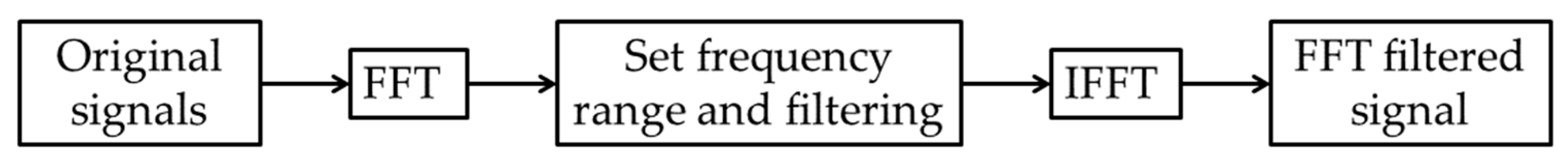
Next, the filtering frequency range is set for the data after FFT, the data within the range are then reserved, and the data outside the range are set to zero. Finally, the inverse FFT operation is executed, that is
The FFT filtering flow chart is shown in Figure 1.

Figure 1.
The working FFT flow chart.
3. Experiments
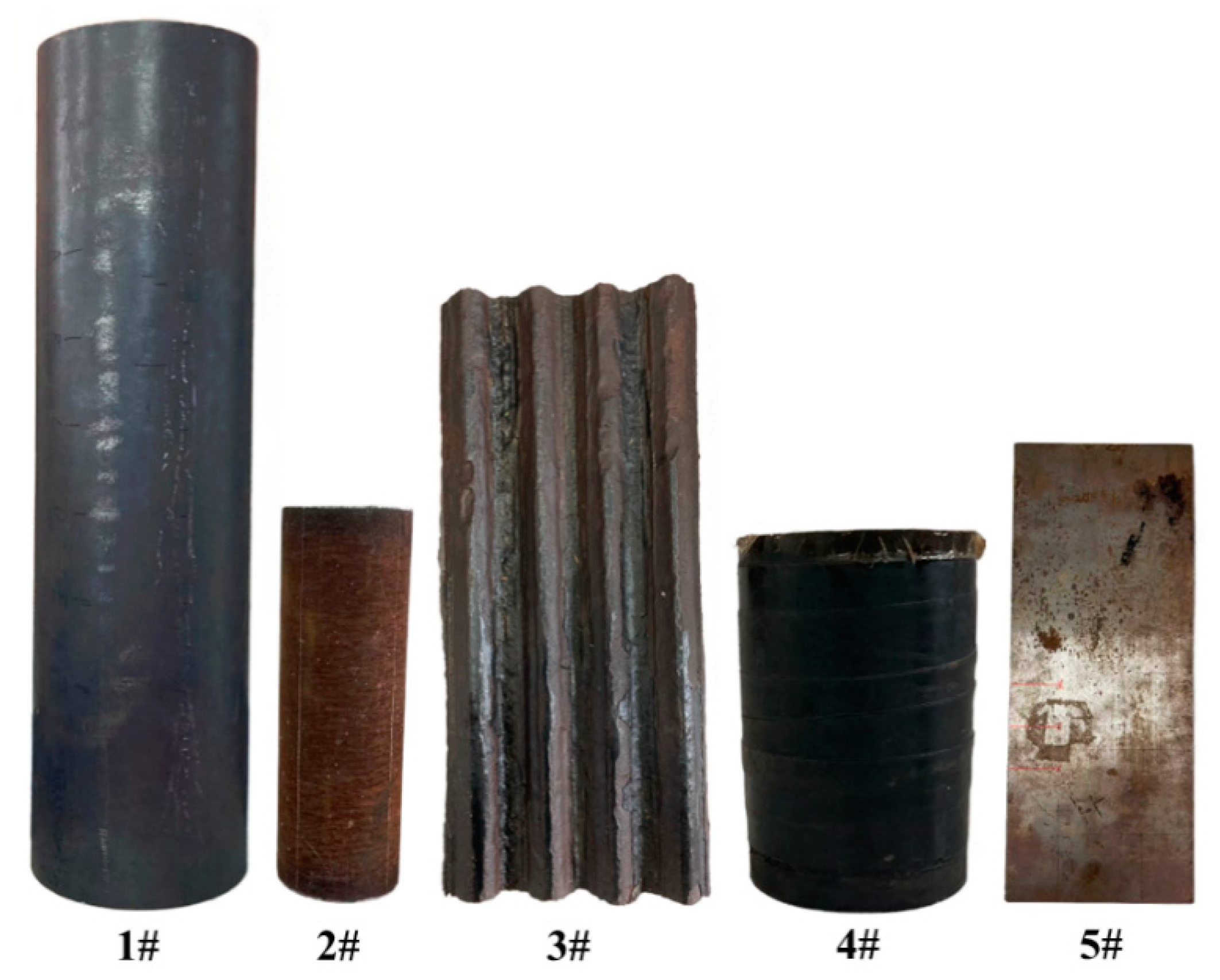
In order to verify the effectiveness of the proposed method, an experimental platform was built as shown in Figure 2. Five different testing specimens were used, the parameters being listed in Table 1. All the specimens were made of carbon steel with different rough and rusty surfaces, as shown in Figure 3. In order to verify the effectiveness of the proposed method for test applications with a certain lift height, the surface of specimen #4 has a 2 mm cladding. A transverse wave EMAT was used to measure the samples; the EMAT was connected to the pulse generator (RPR4000 made by Ritec Corp.) for ultrasonic excitation and reception. A burst pulse signal with an excitation frequency of 1.5 MHz and a single pulse number were set, and the system functioned in pulse-echo mode. The output signals were recorded using a DPO3012 oscilloscope. Using the above theoretical formulation, the SMO–UKF program was written in MATLAB for subsequent data processing.
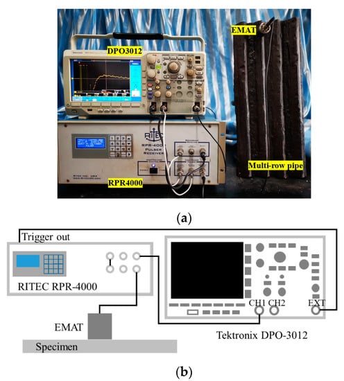
Figure 2.
(a) Photo of experimental setup; (b) Schematic diagram of EMAT testing system.

Table 1.
Specimen parameters (unit: mm).

Figure 3.
Schematic diagram of EMAT testing system.
3.1. Comparison Experiments for Different Specimens
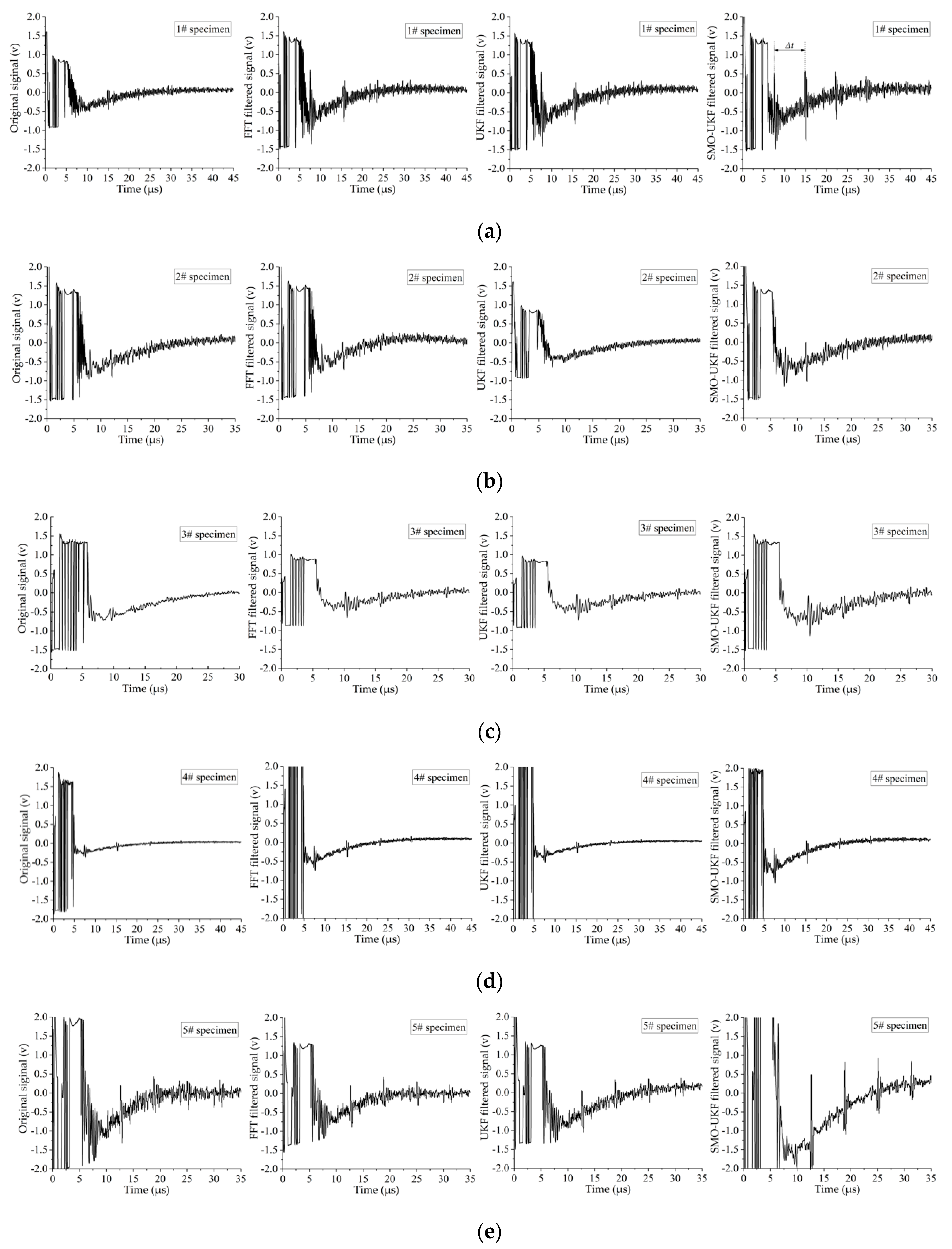
First, the experiments were conducted on all five specimens; the original signals collected are shown in Figure 4 which demonstrates that, except for steel plate #3, the signal-to-noise ratio (SNR) of the other signals are poor. Only the first reflected echo could be found, with the remaining echoes being drowned in the noise.
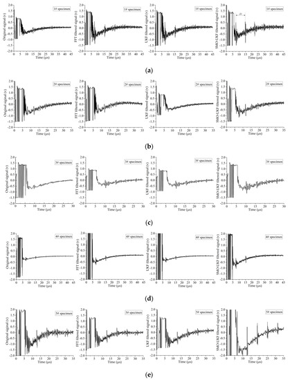
Figure 4.
Comparison before and after filtering by FFT, UKF, and SMO–UKF for: (a) specimen #1 (b) specimen #2, (c) specimen #3, (d) specimen #4, and (e) specimen #5.
The original signals and filtered signals of the five specimens are shown in Figure 4a–e, respectively. The signals in each row from left to right are the original signal, the FFT filtered signal, the UKF filtered signal, and the SMO–UKF filtered signal. It can be observed that the SNRs of the filtered signals are significantly improved, with the echo signals of the SMO–UKF being more obvious.
Since all the reflected echo signals from the inner surface of the pipe emerged from the noise, the interval time between adjacent echoes can be acquired to calculate the wall thickness d; the calculation formula is shown as
where v is the ultrasonic speed of the pipe and ∆t is the interval time, as shown in Figure 4.
The same experiments and signal-processing method were then used for all specimens, #1~#5, and a good gain effect was obtained. In order to verify the detection accuracy of the above method, a vernier caliper and a piezoelectric probe (5 MHz natural frequency, double crystals, 6 mm OD) were also used to measure the five specimens at the same testing points; the results are shown in Table 2. Since the piezoelectric probe was incapable of measuring the steel pipe with cladding, the corresponding result is missing. The echo waves of the original signals for specimens #1 and #2 were difficult to find, so these results are also missing.
Table 2.
Comparison results for different specimens (unit: mm).
Taking the measured value of the Vernier caliper as the true value, the relative error of the calculation results measured by the piezoelectric probe, EMAT, and filtered by FFT, UKF, and SMO–UKF, are calculated and the values appear in parentheses in Table 2. It was found that, after the proposed SMO–UKF method, the signals have a better SNR, demonstrating that a better measurement accuracy was acquired.
3.2. Hyper Parameter Self-Regulation Experiment
In the processing of the above test results, the hyper parameters controlling the Kalman filter gain were manually adjusted. The validation experiments on the automatic hyper parameter adjustments were then carried out. In order to determine the magnitude relationship between Q and R, five cases were assumed and listed, respectively, as: R >> Q (a difference of more than 100 times), R > Q (a difference of 10 to 100 times), R ≈ Q (a difference of 1 to 10 times), R < Q, and R << Q. According to the above relationships, the values of Q and R were assigned, as shown in Table 3.
Table 3.
The assignment of R and Q.
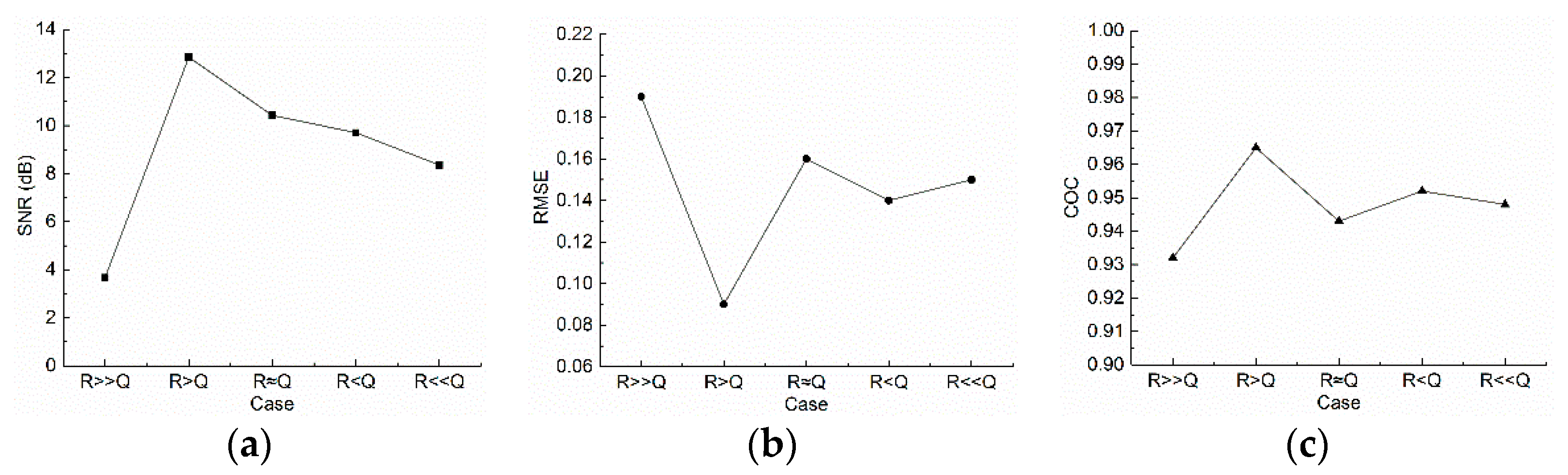
In order to compare the filtering effect of these five assignment cases, several different evaluation indices, such as SNR, root-mean-square-error (RMSE), and correlation coefficient (COC), were used to calculate the filtered data.
SNR represents the ratio between signal power and noise power. The unit of measurement is dB. The larger the signal-to-noise ratio, the smaller the noise mixed in the signal and the higher the signal quality. The calculation formula is:
where, n is the average number, PS is the signal power, PN is the noise power, X (t) is the original signal, and Y (t) is the denoised signal.
RMSE is the square root of the average of the squared sum of the difference between the deviation of each data point from the true value. The smaller the value, the smaller the error, and the better the noise reduction effect. The calculation formula is:
COC indicates the correlation between the denoised signal and the original signal. The larger the correlation coefficient, the better the noise reduction effect. The calculation formula is:
where cov[] and var[], respectively, represent the operations of covariance and variance.
The results are shown in Figure 5. It can be seen that, for different cases, all the RMSEs are around 0.14 and all the COCs are 0.95. While the change of SNR is more obvious, it achieved the maximum value when R > Q. Therefore, in the subsequent self-regulation experiments, R > Q is set as a necessary condition for random assignment, and SNR is used as the optimized evaluation index.
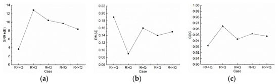
Figure 5.
Using (a) SNR, (b) RMSE, and (c) COC to compare the filtering effect in different magnitude relationships between Q and R.
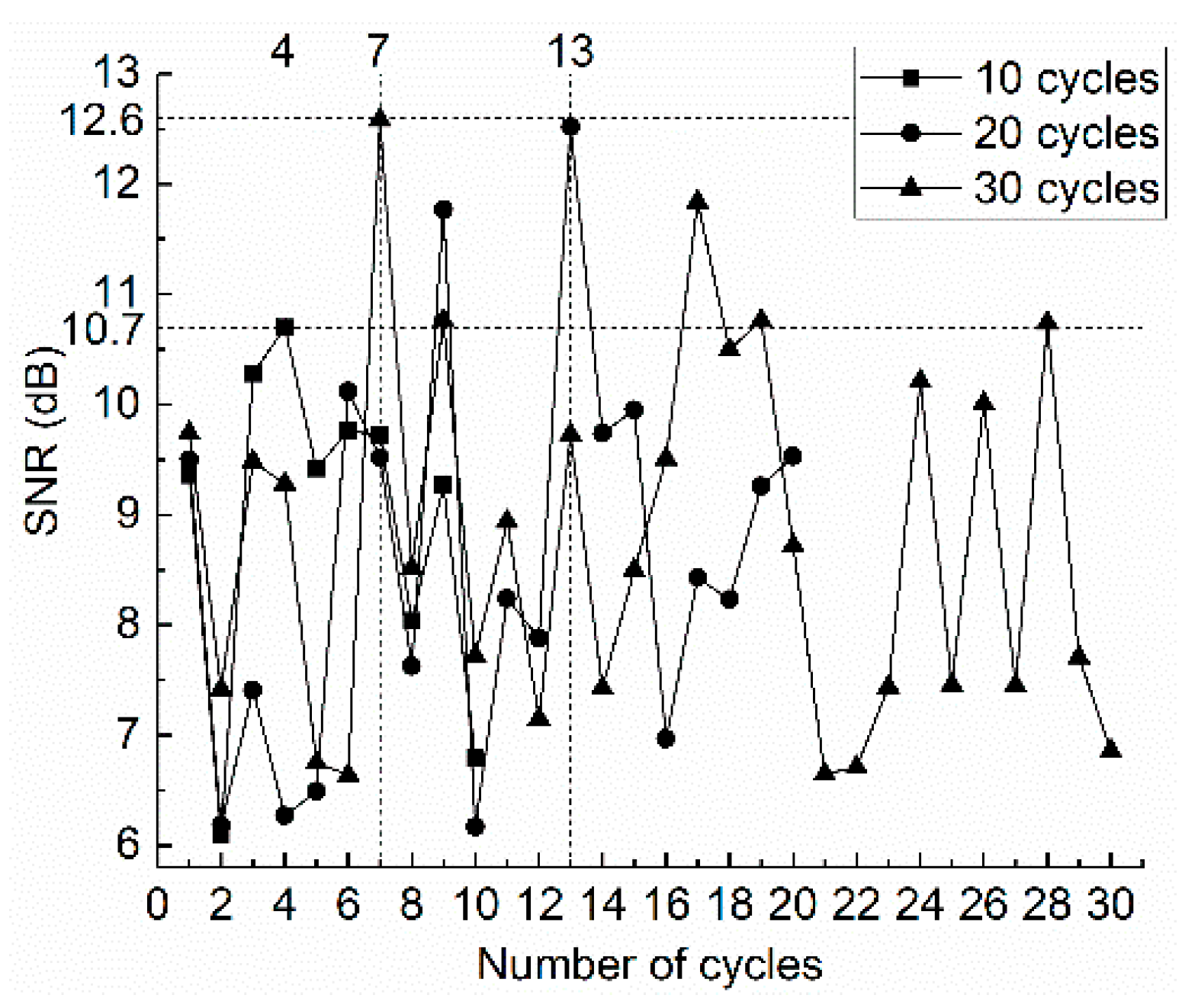
The following random cycle assignment tests were all completed on the row pipe. The value ranges of R and Q were all from 0 to 10, and R > Q. Three groups of cycle experiments were conducted, with the cycle numbers set to 10, 20, and 30, respectively. All testing results were recorded after filtering and are shown in Figure 6.
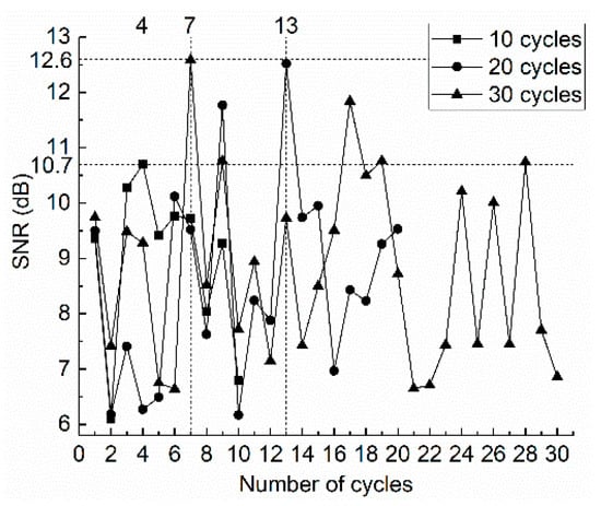
Figure 6.
Comparison of the influence of cycle numbers on SNR.
The testing results demonstrate that the proposed random assignment method can be used to obtain, quickly, a more desirable detection SNR. When cycle numbers n = 10, the best SNR was 10.7 and achieved in the 4th time. The best SNRs were achieved in the 7th and 13th times at n = 20 and n = 30, respectively, and were both 12.6. If the SNR exceeds the value of 10, it is sufficient to calculate the wall thickness in practical applications. Moreover, the increased cycle numbers did not result in any significant improvement in SNR, so a cycle number of 20 is preferred in signal processing.
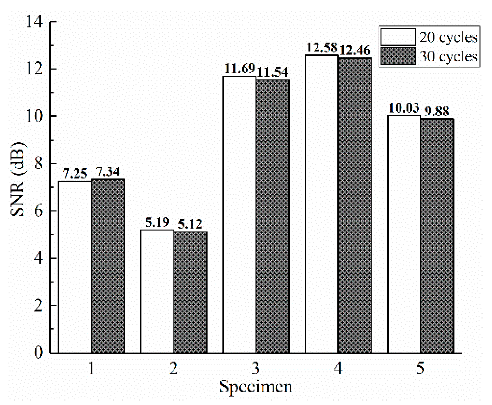
In order to verify the universality of the results, the same testing experiments with 20 and 30 cycle numbers were carried out on specimens #1~#5. The results for the best SNR are shown in Figure 7. Since the surface corrosion conditions of the five specimens were not consistent, the SNRs of the filtered data were not the same, but the maximum SNRs of the five specimens filtered by 20 cycles and 30 cycles were relatively close. This proves that the method of random assignment with finite cycle numbers can quickly accomplish the automatic adjustment of hyper parameters Q and R.
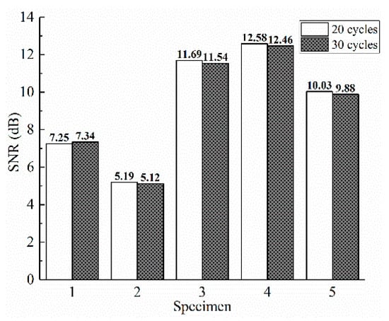
Figure 7.
Testing results for cycle numbers on different specimens.
4. Discussion
4.1. Denoising Effect Analysis
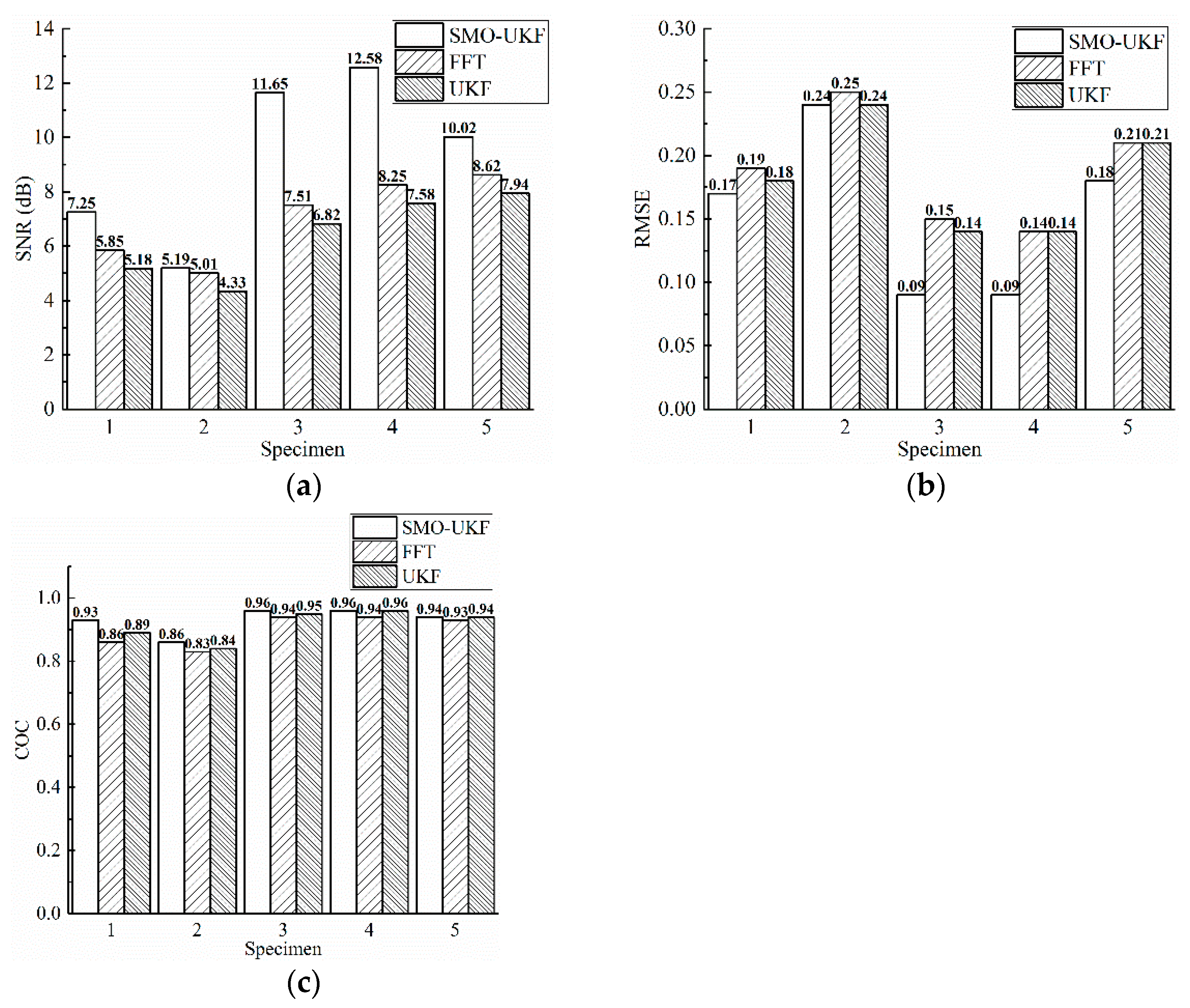
In order to further verify the noise reduction effect of the proposed SMO–UKF filtering algorithm, the inspection data for specimens #1~#5 were used again as samples for comparison and analysis with the UKF filtering algorithm and the classical FFT filtering algorithm, in terms of SNR, RMSE, and COC, respectively; the results are shown in Figure 8.
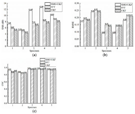
Figure 8.
Denoising effect comparison between UKF, SMO–UKF and FFT: (a) SNR; (b) RMSE; (c) COC.
It can be seen that the SMO–UKF filtering algorithm reduced the noise level of all specimens to a greater extent than did the FFT filtering algorithm. Since the surface corrosion conditions of specimens #1, #2 and #5 are relatively slight, the SNR difference in the two algorithms is small. While the corrosion of specimen #3 is the most serious, the SNR of the testing signal processed by SMO–UKF is 155% and 171% higher compared with processing by FFT and UKF, respectively. It indicates that corrosion has a small influence on the signal frequency components, and the filtering effect by using the FFT algorithm is limited. Although the corrosion of specimen #4 is not critical, the distance between the front end of the probe and the surface of specimen #4 is larger than for other specimens. The SNR also shows increases of 152% and 166%, respectively. The results show that SMO–UKF also has a better effect in eliminating the influence of signal attenuation caused by jitter. The RMSE reflects the average square root of the sum of squares of the differences between each data point and the true value. The smaller the RMSE, the more reliable the measurement. The COC represents the degree of correlation between the denoised signal and the original signal. It can be seen that the signal filtered by SMO–UKF has a high degree of similarity to the original signal, which indicates that the filtering method has good detection accuracy.
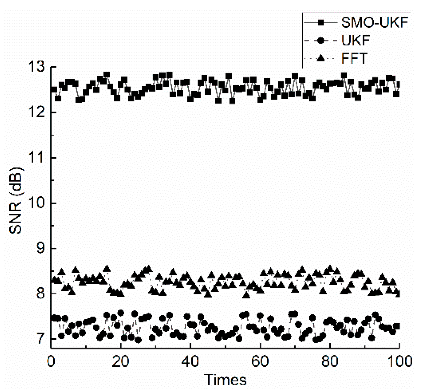
Next, the SMO–UKF, UKF and FFT algorithms were used to repeat filter processing on the test data from specimen #3 one hundred times, and the stability of the three algorithms was compared to the above SNR evaluation index. The test results are shown in Figure 9.
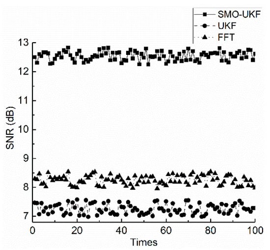
Figure 9.
Denoising stability test with different filtering methods.
It is clear that the signal processed by SMO–UKF had the highest SNR, which proves that the filtering effect of SMO–UKF is significantly better than either the FFT or UKF filtering methods. It has good robustness and can resist the uncertainty of process and measurement noise covariance matrix. In addition, without an observer, the UKF-only filtering method requires a considerable amount of data to obtain a good filtering effect. However, FFT filtering method is carried out by different frequencies, so the effect of UKF is worse than FFT for the same amount of data.
4.2. Computational Efficiency Analysis
The data were filtered using a laptop computer with the Win10 system, an Intel Core I5-5200U processor, a memory capacity of 4 GB, and a hard disk capacity of 1 TB. The computing times for the three filtering methods are shown in Table 4. Compared with the conventional UKF method, the proposed SMO–UKF method can reduce the running time to only 6.4 s, which greatly improves the computational efficiency.
Table 4.
Comparison of computing time of three filtering algorithms.
From the filtering principle, the traditional unscented Kalman filter becomes inaccurate in predicting the state when the dynamic model cannot be accurately expressed, and a large amount of measurement data are needed to make the dynamic model more accurate when filtering; this is the main reason for the high consumption of computing time. In contrast, the approach used in this paper is to continuously estimate the dynamic model error and correct the UKF filtering process by means of a sliding observer; this does not require a large amount of test data and effectively reduces the time consumed during multiple cycles of computing. More importantly, the method used in this paper is more accurate than methods that use a large number of data corrections and consume a considerable amount of computing time.
5. Conclusions
This paper proposes a new SMO–UKF for signal processing in electromagnetic ultrasonic testing to address the performance degradation due to the dynamic model errors involved. The SMO–UKF employs the concept of SMO to improve the UKF adaptiveness and to further resist the effect of dynamic model error on forecast status. It corrects the UKF sensitivity to dynamic model error in the filtering procedure through the estimation and compensation of the error online. Thus, the SMO–UKF overcomes the limitations of UKF and is a promising tool for providing reliable filtering results for systems in the presence of dynamic model error. The calculation results demonstrate that the SNR of the testing EMAT signals, processed by the proposed SMO–UKF, had a maximum increase of 155% and 171% relative to FFT and UKF, respectively. Through the experimental tests, it was determined that when R was greater than Q, and their values ranged from 0 to 10, a better Kalman filter effect was obtained. In the process of Kalman filtering, the self-regulation function was added to assign hyper parameters to reduce the need for manual assistance and greatly reduce the running time to only 6.4 s.
Author Contributions
Conceptualization, X.S.; methodology, Q.W.; software, H.Z.; validation, H.Z. and Z.D.; investigation, C.C.; resources, J.T.; writing—original draft preparation, H.Z.; writing—review and editing, J.T.; supervision, J.T.; project administration, X.S.; funding acquisition, J.T. and Z.D. All authors have read and agreed to the published version of the manuscript.
Funding
This research was funded by the Key Research and Development Plan Project, Hubei Province (Grant No. 2022BAA075); the National Natural Science Foundation of China (Grant No. 52105550); and the Green Industrial Science and Technology Leading Project at Hubei University of Technology (Grant No. CPYF2018006).
Institutional Review Board Statement
Ethical review and approval were waived for this study is not involving humans or animals.
Informed Consent Statement
Patient consent was waived for this study is not involving humans.
Data Availability Statement
Not applicable.
Conflicts of Interest
The authors declare no conflict of interest.
References
- Sun, H.Y.; Peng, L.S.; Huang, S.L. Microcrack Defect Quantification Using a Focusing High-Order SH Guided Wave EMAT: The Physics-Informed Deep Neural Network GuwNet. IEEE Trans. Ind. Inform. 2021, 18, 3235–3247. [Google Scholar] [CrossRef]
- Cai, Z.C.; Zhao, Z.Y.; Chen, L.; Tian, G.Y. Optimal design of shear vertical wave electromagnetic acoustic transducers in resonant mode. Int. J. Appl. Electromagn. Mech. 2020, 64, 639–647. [Google Scholar] [CrossRef]
- Zhao, X.; Liu, Z.; Guo, Y.; He, C.; Wu, B. An Advanced Magnetoacoustic Compound Inspection Method of High-Order Mode EMAT. IEEE Sens. J. 2022, 22, 229–239. [Google Scholar] [CrossRef]
- Oruklu, E.; Saniie, J. Hardware-efficient realization of a real-time ultrasonic target detection system using IIR filters. IEEE Trans. Ultrason. Ferroelectr. Freq. Control. 2009, 56, 1262–1269. [Google Scholar] [CrossRef]
- Abbate, A.; Koay, J. Signal detection and noise suppression using a wavelet transform signal processor: Application to ultrasonic flaw detection. IEEE Trans. Ultrason. Ferroelectr. Freq. Control 1997, 44, 14–26. [Google Scholar] [CrossRef]
- Ding, Y.; Reuben, R.L.; Steel, J.A. A new method for waveform analysis for estimating AE wave arrival times using wavelet decomposition. NDT & E Int. 2004, 37, 279–290. [Google Scholar] [CrossRef]
- Tarpara, E.G.; Patankar, V.H. Real time implementation of empirical mode decomposition algorithm for ultrasonic nondestructive testing applications. Rev. Sci. Instrum. 2018, 89, 125118. [Google Scholar] [CrossRef]
- Shi, Z.M.; Liu, L.; Peng, M.; Liu, C.C.; Tao, F.J.; Liu, C.S. Non-destructive testing of full-length bonded rock bolts based on HHT signal analysis. J. Appl. Geophys. 2018, 151, 47–65. [Google Scholar] [CrossRef]
- Pedram, S.K.; Fateri, S.; Gan, L. Split-spectrum processing technique for SNR enhancement of ultrasonic guided wave. Ultrasonics 2018, 83, 48–59. [Google Scholar] [CrossRef]
- Abbate, A.; Frankel, J.; Das, P. Wavelet transform signal processing for dispersion analysis of ultrasonic signals. IEEE Ultrason. Symp. 1995, 1, 751–755. [Google Scholar] [CrossRef] [Green Version]
- Huang, N.E.; Shen, Z.; Long, S.R. The empirical mode decomposition and the Hilbert spectrum for nonlinear and nonstationary time series analysis. Proc. R. Soc. Lond. 1998, 454, 903–995. [Google Scholar] [CrossRef]
- Newhouse, V.L.; Bilgutay, N.M.; Saniie, J. Flaw-to-grain echo enhancement by split-spectrum processing. Ultrasonics 1982, 20, 59–68. [Google Scholar] [CrossRef]
- Sun, F.; Hu, X.; Yuan, Z. Adaptive unscented Kalman filtering for state of charge estimation of a lithium-ion battery for electric vehicles. Fuel Energy Abstr. 2014, 36, 3531–3540. [Google Scholar] [CrossRef]
- Wang, S.; Kang, L.; Li, Z.; Zhai, G.; Zhang, L. 3-D modeling and analysis of meander-line-coil surface wave EMATs. Mechatronics 2012, 22, 653–660. [Google Scholar] [CrossRef]
- Liu, Z.H.; Deng, L.M.; Zhang, Y.C.; Li, A.L.; Wu, B.; He, C.F. Development of an omni-directional magnetic-concentrator-type electromagnetic acoustic transducer. NDT&E Int. 2020, 109, 102193. [Google Scholar] [CrossRef]
- Tu, J.; Chen, T.; Xiong, Z.; Song, X.C.; Huang, S.L. Calculation of Lorentz force in planar EMAT for thickness measurement of steel plate. Int. J. Comput. Math. Electr. Electron. Eng. 2017, 36, 1257–1269. [Google Scholar] [CrossRef]
- Soken, H.E.; Hajiyev, C. Adaptive fading UKF with Q-Adaptation: Application to pico satellite attitude estimation. J. Aerosp. Eng. 2013, 26, 628–636. [Google Scholar] [CrossRef]
- Cho, S.Y.; Choi, W.S. Robust positioning technique in low-cost DR/GPS for land navigation. IEEE Trans. Instrum. Meas. 2006, 55, 1132–1142. [Google Scholar] [CrossRef]
- Zhang, L.; Zhu, Y.; Shi, P. Resilient Asynchronous H∞ filtering for markov jump neural networks with unideal measurements and multiplicative noises. IEEE Trans. Cybern. 2015, 45, 2840–2852. [Google Scholar] [CrossRef]
- Hu, G.; Ni, L.; Gao, B. Model predictive based unscented Kalman filter for hypersonic vehicle navigation with INS/GNSS integration. IEEE Access 2020, 8, 4814–4823. [Google Scholar] [CrossRef]
- Song, X.; Fang, J.; Han, B. Adaptive compensation method for high-speed surface PMSM sensorless drives of EMF-based position estimation error. IEEE Trans. Power Electron. 2016, 31, 1438–1449. [Google Scholar] [CrossRef]
- Jin, S.; Kikuuwe, R.; Yamamoto, M. Real-time quadratic sliding mode filter for removing noise. Adv. Robot. 2012, 26, 877–896. [Google Scholar] [CrossRef]
- Fan, C.G.; Pan, M.C.; Luo, F.L. Ultrasonic broadband time-reversal with multiple signal classification imaging using full matrix capture. Insight Non-Destr. Test. Cond. Monit. 2014, 56, 487–491. [Google Scholar] [CrossRef]
- Brigham, E.O. The Fast Fourier Transform; Prentice Hall: Englewood Cliffs, NJ, USA, 1974. [Google Scholar]

Publisher’s Note: MDPI stays neutral with regard to jurisdictional claims in published maps and institutional affiliations. |
© 2022 by the authors. Licensee MDPI, Basel, Switzerland. This article is an open access article distributed under the terms and conditions of the Creative Commons Attribution (CC BY) license (https://creativecommons.org/licenses/by/4.0/).