Article

Analysis of Leaked Crude Oil in a Mountainous Area

Beijing Key Laboratory of Process Fluid Filtration and Separation, College of Mechanical and Transportation Engineering, China University of Petroleum-Beijing, Beijing 102249, China
*
Author to whom correspondence should be addressed.
Energies 2022, 15(18), 6568; https://doi.org/10.3390/en15186568
Submission received: 5 August 2022 / Revised: 31 August 2022 / Accepted: 5 September 2022 / Published: 8 September 2022
(This article belongs to the Special Issue Fundamentals and Applications of Multiphase Flow and Heat Transfer)

Abstract

:
China–Myanmar oil and gas pipelines in Southwest China guarantee the energy security of China. Due to poor geographical circumstances, the safety of pipelines is seriously threatened by natural disasters. Therefore, there is a crucial, practical significance to establishing a model of leakage and diffusion of crude oil in the mountainous terrain and to conduct related applied studies. In the present study, computational fluid dynamic simulations of the dynamic diffusion process of leaking contaminants on the mountain surface was performed; the influence of the pipe pressure, landform, surface environment and leakage location on diffusion speed and range were discussed carefully. The results indicate that the variation of topographic altitude determines the path of leaking contaminants. Accordingly, an improved algorithm based on the SFD8 algorithm to predict the path of leaking contaminants at a low leakage rate was proposed; this would be instructive for an emergency response to ensure the safety of pipelines.

1. Introduction

Sino–Myanmar pipelines, with a designed transmission capacity of 22 million tons of crude oil per year, have already become a key energy artery for China [1,2,3]. A survey of the entire pipeline shows that the maximum altitude drop reaches approximately 2000 m, the construction in the mountainous area accounts for 81% and it passes through 12 rivers and 64 mountain tunnels. The domestic regions where the pipeline passes through are characterized by highly complicated terrain. The severe natural and geographical environment in the mountains of Southwest China poses a tremendous potential threat to the safety of the pipeline. The frequent occurrence of natural disasters, such as earthquakes, debris flow and landslide cause the exposure, displacement and fracture of pipelines [4,5]. Consequently, leaked crude oil spreads rapidly across the mountain surface, leading to large-scale soil deterioration and groundwater resource pollution [6]. Therefore, profound knowledge of the path and diffusion of leaked crude oil in a mountainous area is of utmost importance for severe accident management.
So far, extensive studies have been carried out to describe the diffusion patterns and range of the spilled oil under various operations and surface conditions. Briscoe and Shaw [7] proposed the SPILL model under the conditions of instantaneous leakage and continuous leakage, according to the Fay equation [8], to describe the diffusion behavior of the leaked liquid on a permeable surface. However, the influence of ground roughness and terrain conditions on the diffusion of the liquid pool are ignored, resulting in a large deviation between the calculation results and the actual situation. In order to overcome the defects of this model, some scholars have improved it: Kapias et al. [9,10,11] established a liquid pool model to simulate the diffusion behavior of the leaked liquid and predict the thickness of the liquid pool; Webber et al. [12] established a surface diffusion model based on the shallow water wave equation, which can simulate the diffusion process under three different surface conditions of smooth ground, rough ground and water surface; Witlox et al. [13] determined the diffusion radius of the liquid pool in the final state by introducing the law of diffusion so that the calculation result is closer to the actual situation.
There are some existing studies that focus on buried pipeline leakage accidents. Scholars such as Wu et al. [14] and Ji et al. [15] studied the motion characteristics of oil in the porous soil, revealing that factors such as the volume of leaked oil, phase transition of oil, soil pore diameter, pipeline depth, temperature and the viscosity of oil will make a difference for buried oil pipeline leakage accidents. He et al. [16] investigated the characteristics of dynamic seepage-diffusion of leaked oil in porous soil, and analyzed the effects of the pressure transmission coefficient, the leak orifice’s size, the leakage flowrate, pipe diameter and the leak orifice’s position. Norouzi et al. [17] also explored the effect of the capillary number on the immiscible fluid displacement in porous media by a simulation with the LBM method; the results show that with an increase in the capillary number, the viscous force becomes predominant.
Besides studies that focus on buried pipeline leakage accidents, studies about the motion of spilled oil on the ground have been carried from other scholars. The flow of spilled oil on the ground can be simplified as the problem of the spread of fluid spilled on a flat or inclined surface. Cavanaugh et al. [18] studied the leakage accidents of oil storage tanks on flat ground, and they calculated the diffusion and volatilization laws of the oil leaked from the oil storage tanks on the flat surface with the LSM90 model; Tauseef et al. [19] summarized many empirical formulas that calculate the diffusion range of italic spills, including the empirical formula for continuous liquid spilling (Bachelor proposed in 1967, the Raisbeck and Mohtadi model was proposed in 1974) and the empirical formula for intermittent liquid spillage (the Hussein model was proposed in 2002, the Simmons model was proposed in 2004, the Benfer model was proposed in 2010 [20], the Meel and Khajehnajafi model was proposed in 2012). These empirical formulas for calculating the liquid spill problem can predict the final diffusion area of the spilled liquid through parameters such as the physical properties of the spilled fluid, the ambient temperature, the properties of the ground and the evaporation rate. Raja et al. [21] compared various empirical formulas that calculate the spillage of leaking fluid with experimental results; they verified the accuracy of each formula and provided a large number of empirical formulas that can be used to calculate the diffusion range of spilled liquids; Hussein et al. [22] analyzed the force during the diffusion process of the flow on the plane, and summarized the effects of gravity, tension and viscous force on the flow when the fluid was spilled on the plane. At the same time, the possible evaporation of the leaking fluid in the open air is also taken into account.
In addition, there are some scholars that focus on the oil diffuse process on the water surface. Blokker et al. [23] took the expansion of oil film on the free plane as the premise, took gravity as the driving force in the process of oil film expansion, and ignored the viscous force and surface tension in the process of oil film expansion; they finally obtained the inertial expansion process of the oil film under the action of tension. Fay et al. [8] proposed the Fay theory, which more comprehensively considered the gravity, viscous force, surface tension and inertial force of the oil film on the water surface during the diffusion process.
In the follow-up research, scholars such as Al-Rabeh et al. [24] and Karafyllidis et al. [25] simulated the oil leakage by considering the oil leakage as countless oil particles, and assigned a random variable value with weight to the movement speed of each oil particle to simulate the diffusion process of oil spills on the water surface; Lehr et al. [26] and other scholars took into account the influence of water flow and air movement on the water surface oil film movement. Geng et al. [27] found, through theoretical formula derivation and experimental analysis, that the calculation of the oil film expansion movement on the surface of water is further improved by the theoretical formula.
It should be noted that previous studies in this field have significant reference. However, the above models have not considered the effect of actual topographical conditions on the diffusion process of the leaked crude oil. To the best of our knowledge, there is no relative study on the path and diffusion of leaked crude oil in a mountainous area.
In the present study, the aim is to gain a better understanding of the dynamic diffusion process of leakage contaminants on the mountain surface and to develop an algorithm to predict the path of leaking contaminants. In order to resolve the phase interface satisfactorily, the standard volume-of-fluid (VOF) technique is used, and high-quality tetrahedral grids are developed for the computational domain. The effects of leaking velocity, surface conditions and terrain features are analyzed in detail. By analyzing the numerical simulation results, an improved algorithm based on the SFD8 algorithm to predict the path of leaking contaminants at a low leakage rate is proposed.

2. Computational Approach

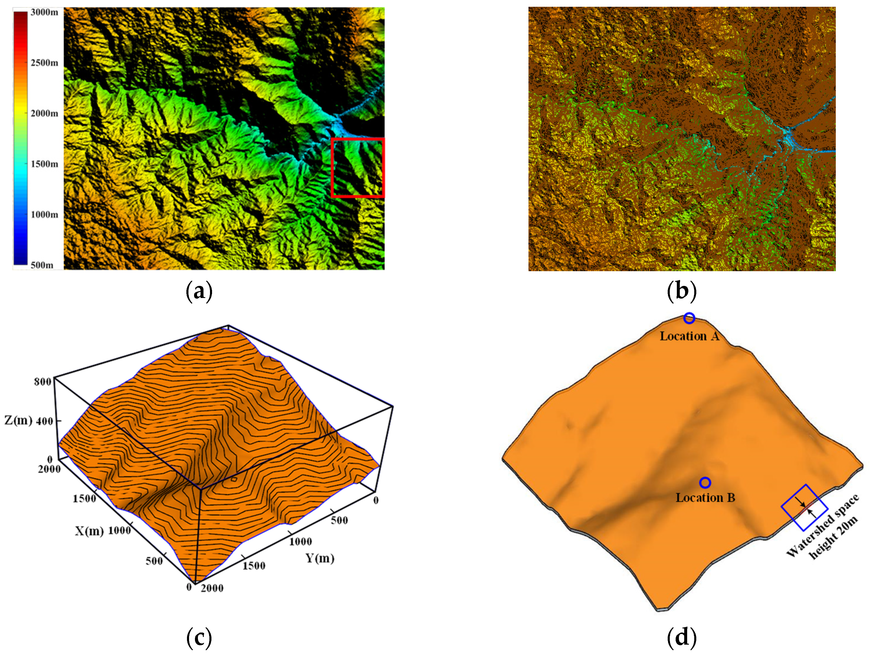
2.1. Computational Domain

Topographic features of a typical natural terrain located in the Yunnan Province of China are extracted to investigate the diffusion patterns (see Figure 1a). The Global Mapper is employed to convert terrain features into a series of contour lines (see Figure 1b) and then create a three-dimensional natural terrain surface by Sketchup (see Figure 1c) [28]. The size of the mountain is 2000 m (long) × 2000 m (wide) × 800 m (height). The diameter of the pipe is 0.8 m, and it is assumed that the direction of the jet at the early stage of the leakage is parallel to the mountain surface. Accordingly, a computational domain with a height of 100 m above the mountain surface is built, as illustrated in Figure 1d. A leakage occurring in both a valley (location A with a height of 800 m) and ridge (location B with a height of 400 m) is taken into consideration in the present study. Locations A and B are chosen for the purpose to investigate different diffusion patterns with different topographic characteristics; positions A and B, respectively, represent typical topographic characteristics of a valley and ridge.

2.2. Grid Construction

Due to the terrain undulation, the surface curvature varies greatly in parts of the areas. Therefore, the tetrahedral grids are deployed to the entire computational domain, as shown in Figure 2 [29]. Ansys software Mesh is used for generating the mesh; it can be seen that the entire computational domain is built according to the ground surface of the mountain. The mesh of the pipeline leak exiting the computational domain is properly encrypted to improve the accuracy of simulation.
A preliminary grid sensitive test is conducted to find the suited grid size. The preliminary grid sensitive test suggests that a grid size of 1 million is sufficient to predict the path of the leaked oil reasonably, and the resolution of captured diffusion is compromised. Thus, the mesh is carefully refined and encrypted for the surface with a large curvature variation. Finally, the number of grids is 1.13 million in total.

2.3. Simulation Settings

Software Fluent is used to simulate the flow process of leaking oil; the air and crude oil are used as the working fluid. According to the parameters of operation and environment of the China–Myanmar pipeline, the initial velocity of the leak is assumed to be 30 m/s, 50 m/s and 80 m/s. The fluid properties are assumed to remain constant during the simulation, i.e., ρ oil = 830 kg/m3, μ oil = 0.00332 kg/m s for crude oil and ρ air = 1.225 kg/m3, μ air = 1.7894 e 5 kg/m s for air.
The PISO (Pressure Implicit with Splitting of Operators) scheme is used to tackle the pressure–velocity coupling. It is a non-iterative algorithm for solving pressure–velocity coupling, proposed by Issa in 1986, and it is also one of the most widely used pressure–velocity decoupling methods.
The standard-k epsilon scheme is used as the viscous model. The moment and turbulent equations are discretized based on a second-order upwind scheme. The volume of fluid (VOF) model is applied to obtain characteristics of three-dimensional open channel flows involving free surfaces on the mountain surface [30]. The phase interface is also constructed by applying a modified High-Resolution Interface Capturing (HRIC) technique. Note that the surface environment has a serious influence on the law of leakage diffusion. In the present study, four kinds of surface environments—termed as a smooth surface, a surface with a degree of roughness and surfaces covered by short grass and shrub—are investigated, as listed in Table 1.
The roughness of different surface conditions can be found in [29]; the values of roughness length and roughness height are data obtained by fitting the empirical formula.
The diffusion of leaked oil in the soil is not captured during this simulation, since the effect of oil subsurface diffusion is decreasing the leak spread area of oil, and the effect grows over time. In our simulation, the flow processes of oil only last dozens of seconds after the damage of the oil pipeline; thus, the effect of diffusion of leaked oil in the soil is negligible, and the simulation only considers the flow and diffusion process of spilled oil on mountain ground surface. No porous media area in the calculation domain was built to describe the properties of the subsurface soil.

3. Simulation Results and Discussion

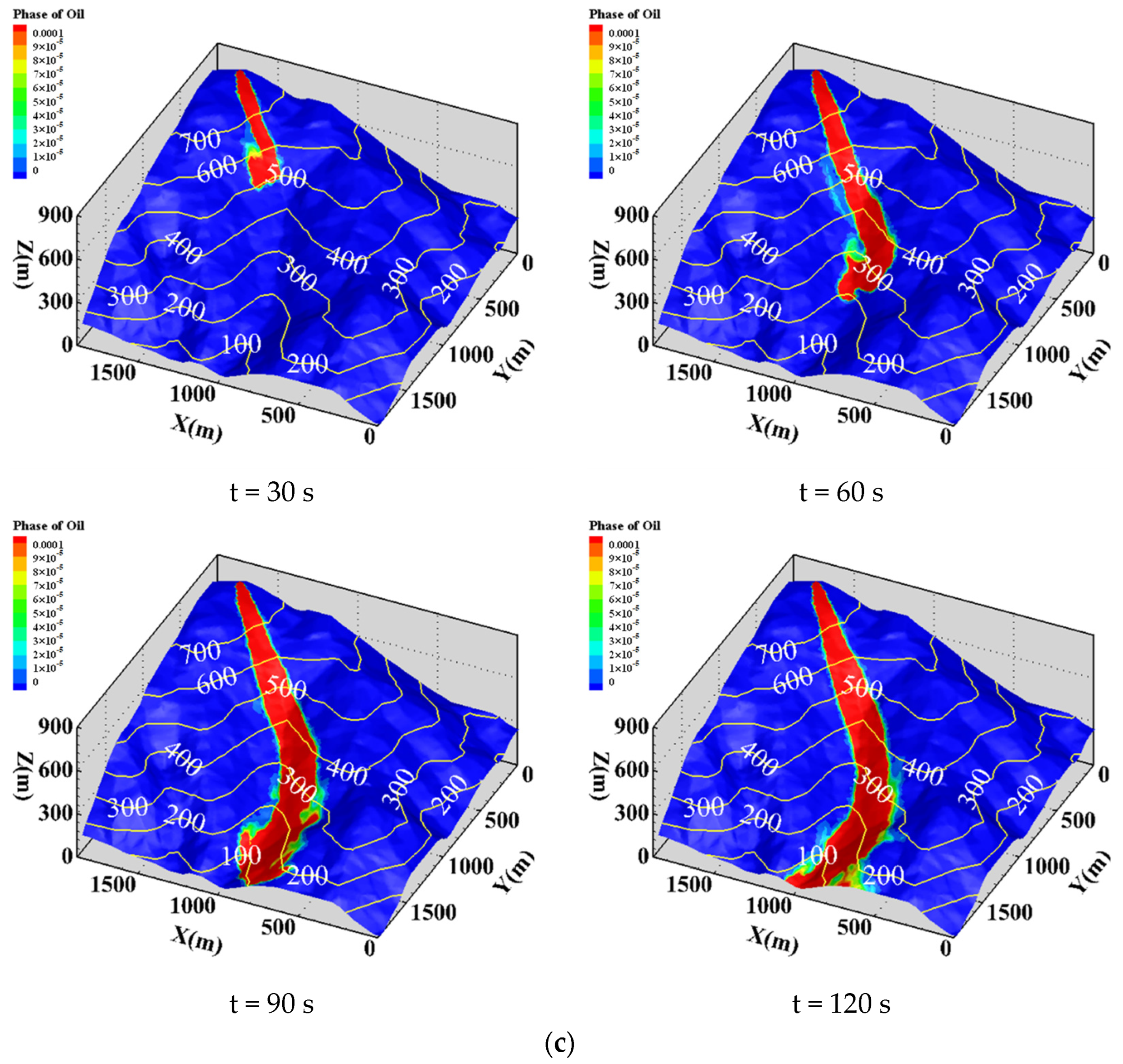
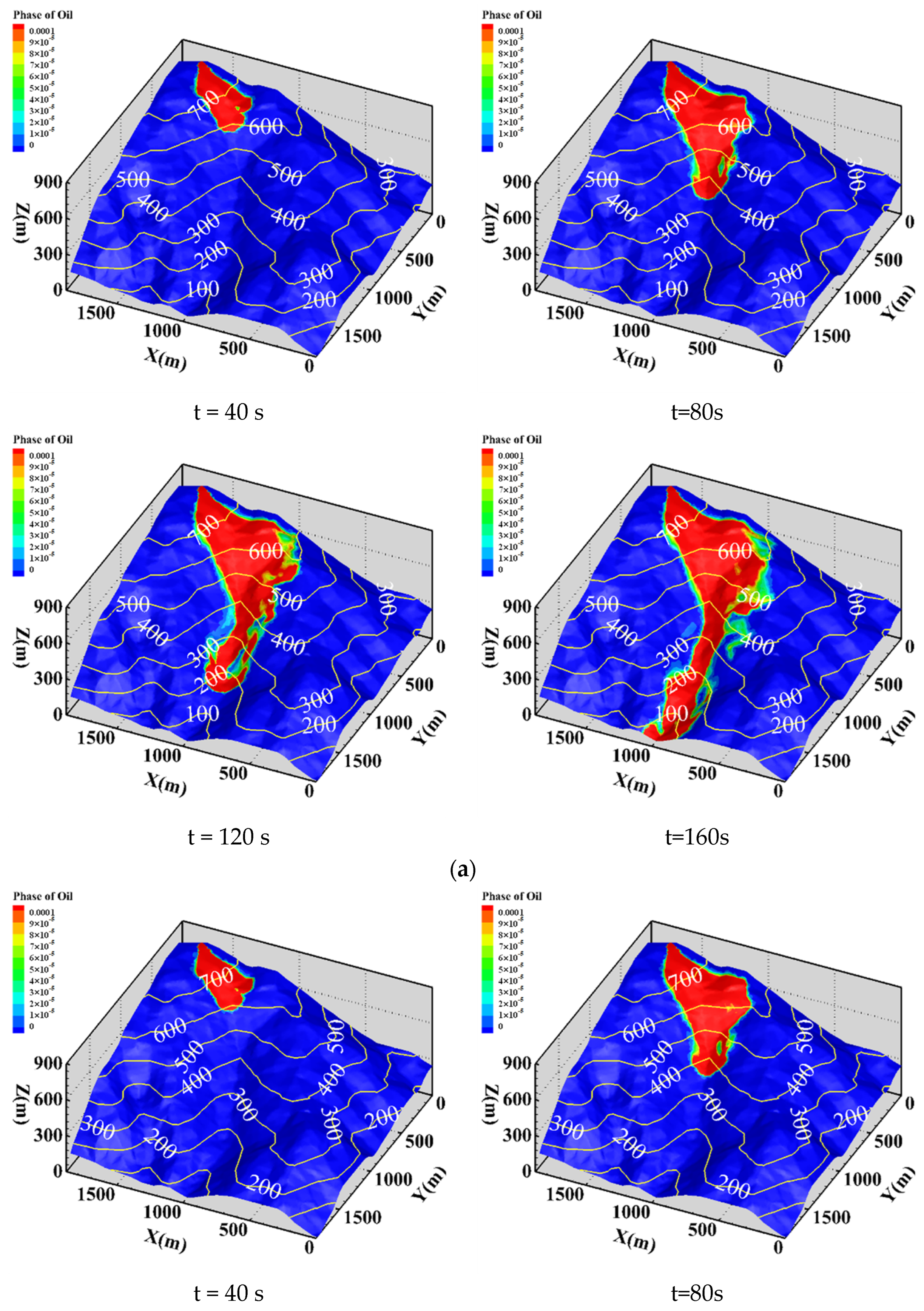
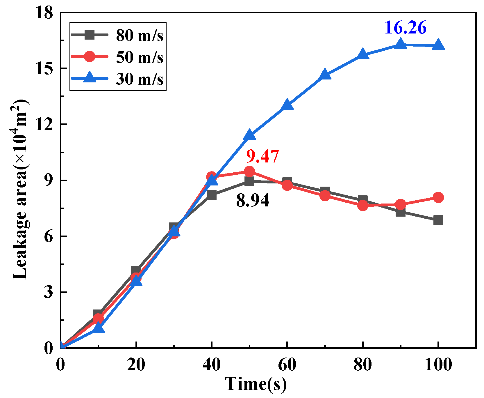
3.1. Leakage in the Valley

After a leakage in the valley, the diffusion patterns of crude oil along a smooth surface at different leakage rates are depicted in Figure 3. At a lower initial leakage velocity of 30 m/s, most crude oil overflows the valley and spreads over the ridge, leading to a reduction in the amount of crude oil flowing along the gully. By increasing the initial leakage velocity to 50 m/s, the crude oil diffuses less laterally on the upper half of the mountain, while it flows more downward along the gully. When the initial leakage velocity reaches 80 m/s, the crude oil is rapidly ejected from the top of the mountain in the form of a jet under the action of high pressure in the tube so that the initial overall flow state is a liquid column. Then, the crude oil changes its flow direction under the obstruction of the gully and flows down the gully to the bottom of the mountain. Figure 4 shows the statistical spread area and flow time to the foot of the mountain. Obviously, increasing the initial leakage velocity reduces the time it takes for the oil to reach the foot of the mountain and the spread area of oil on the mountain surface.
Figure 5 shows the diffusion patterns of leaked crude oil on different mountain surfaces at a constant initial leakage velocity of 50 m/s. Compared with the diffusion pattern on the smooth surface (see Figure 3b), the diffusion ranges of the leaked crude oil on these three surfaces are more extensive. However, the effect of the surface condition on the flow path is negligible. Figure 6 illustrates the statistical spread area and flow time to the foot of the mountain. Accordingly, the surface condition mainly affects the diffusion area of the leaked crude oil. The downward flow is more hindered by higher surface roughness (rough land, short grass and shrub). What is noteworthy is that the spread area on the shrub surface is almost the same as that of the short grass surface. It can be deduced that the average impact height of crude oil does not exceed the roughness height of short grass, thus, there will be no further impact on the leak and diffusion of crude oil when the surface roughness further increases.

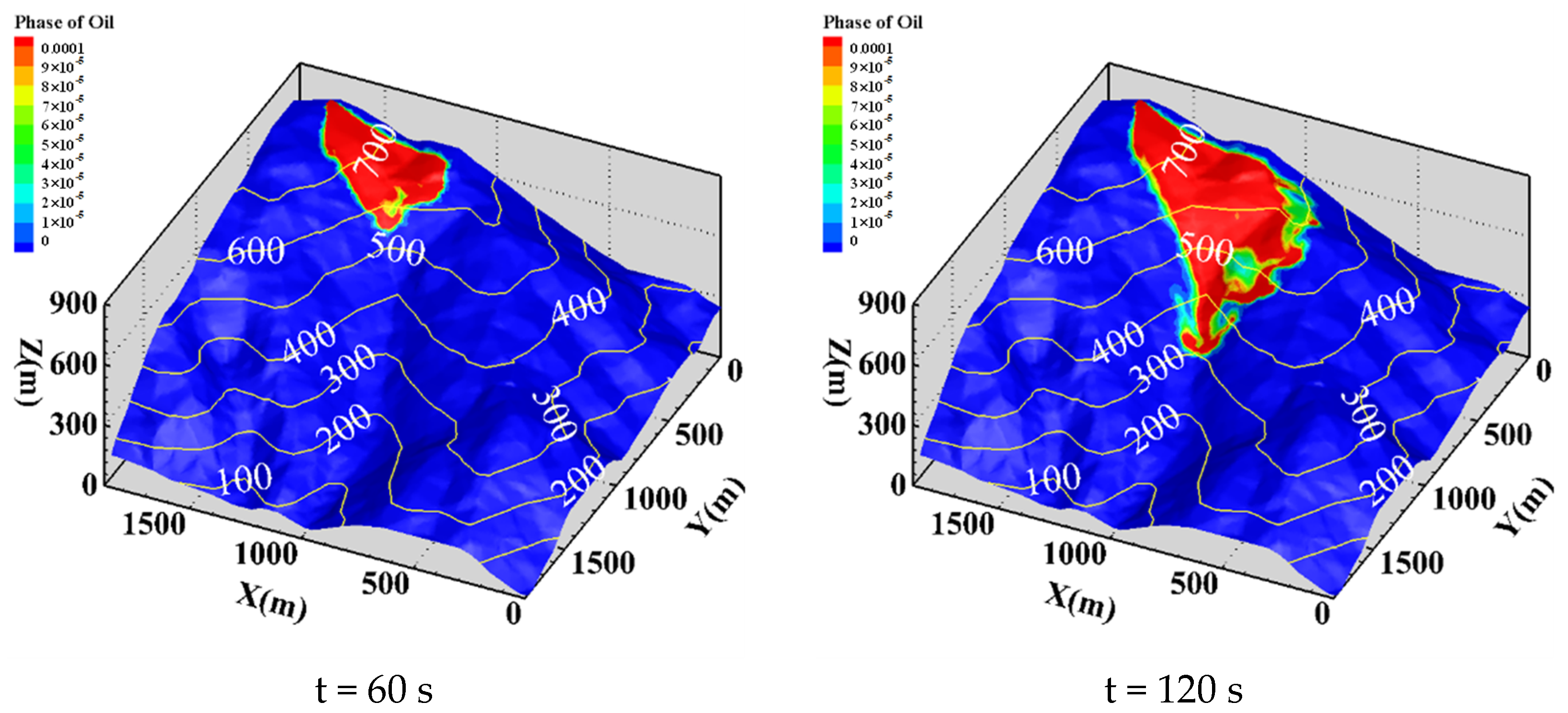
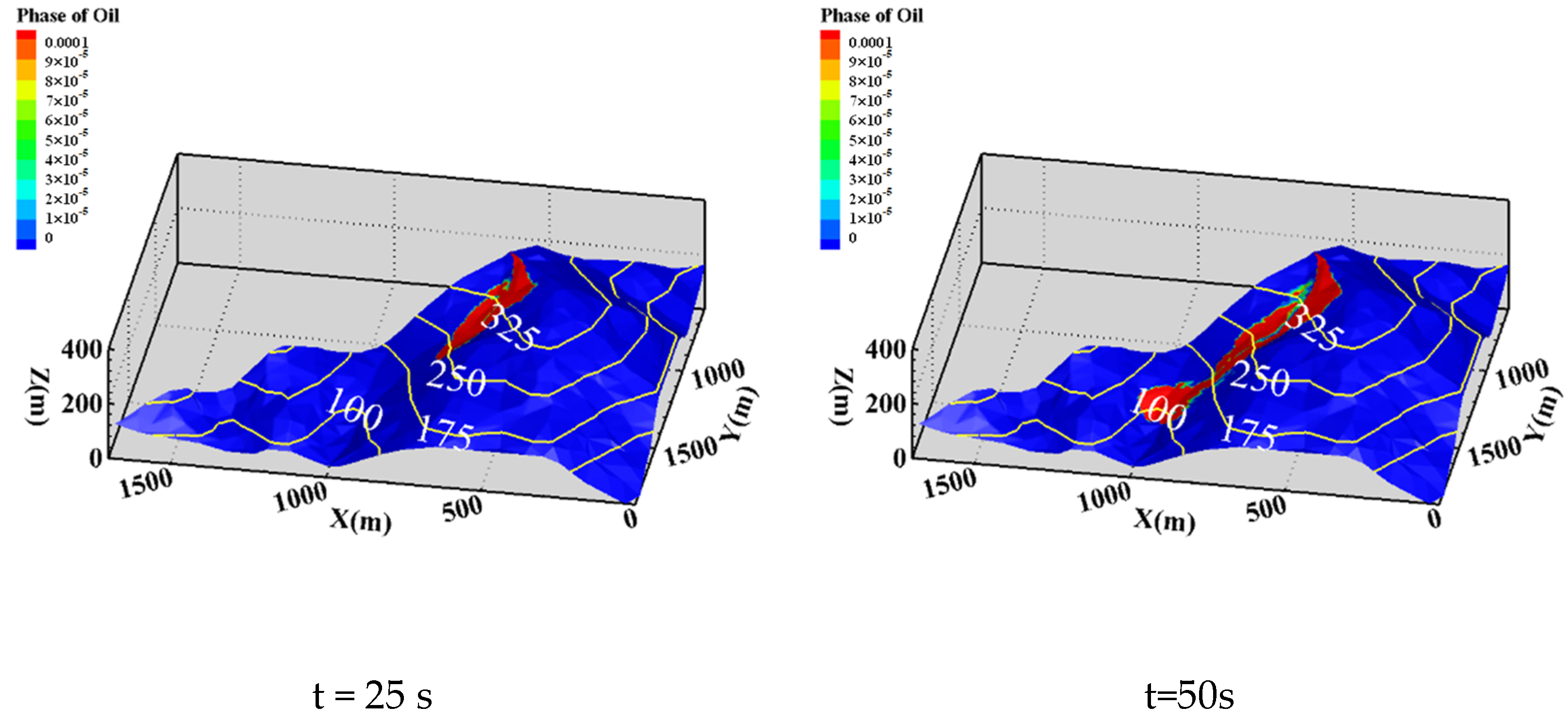
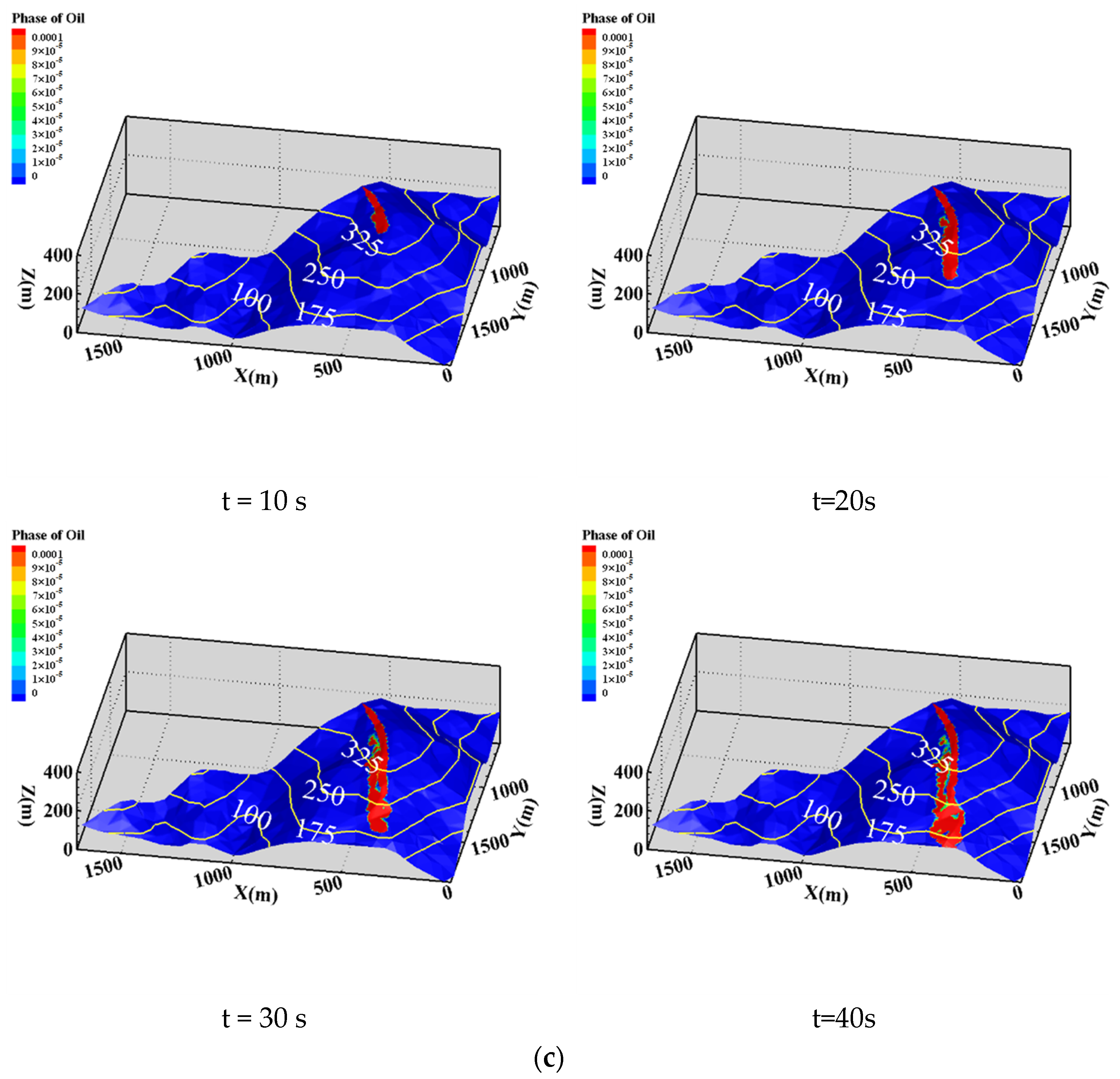
3.2. Leakage at the Ridge

Figure 7 shows the diffusion patterns of leaked crude oil at the mountain ridge under different initial velocities. Compared with the diffusion in the valley, the most distinctive trait of the diffusion pattern is that the direction of flow is closely related to the velocity of the fluid. At a lower initial velocity, the leaked oil tends to flow towards the valley, whereas it tends to flow in the direction of a ridgeline at a higher initial velocity. Figure 8 shows the statistical spread area and flow time to the foot of the mountain. There is no doubt that the spread area of oil on the mountain surface is small compared to the leakage that occurs in location A due to the decrease in altitude. At the same time, when the leakage occurs at the ridge, the crude oil presents an entirely different leak path at different initial velocities, which makes the change-of-spread area with a velocity more unpredictable. Additionally, as the spread area of oil is calculated by the phase fraction of the oil everywhere on the mountain ground surface, the area where the phase fraction of the oil is greater than a certain value will be counted as the oil spread area; thus, the oil will collect over time in some areas, causing the spread area to decrease over time, as shown in the example in Figure 8, with initial velocities of 50 and 80 m/s. The turbulence of the fluid causes the motion of the fluid to have a certain randomness; therefore, the value of the spread area will fluctuate to some extent.

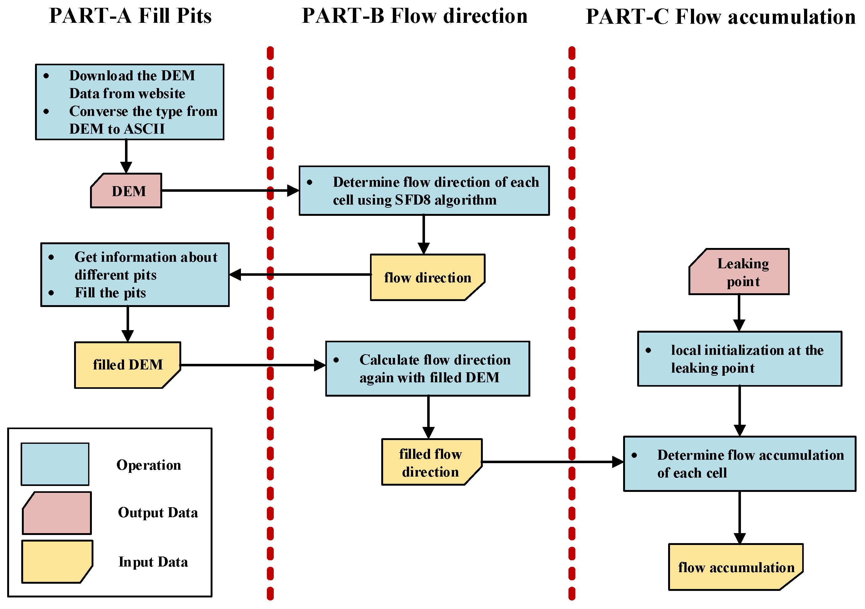
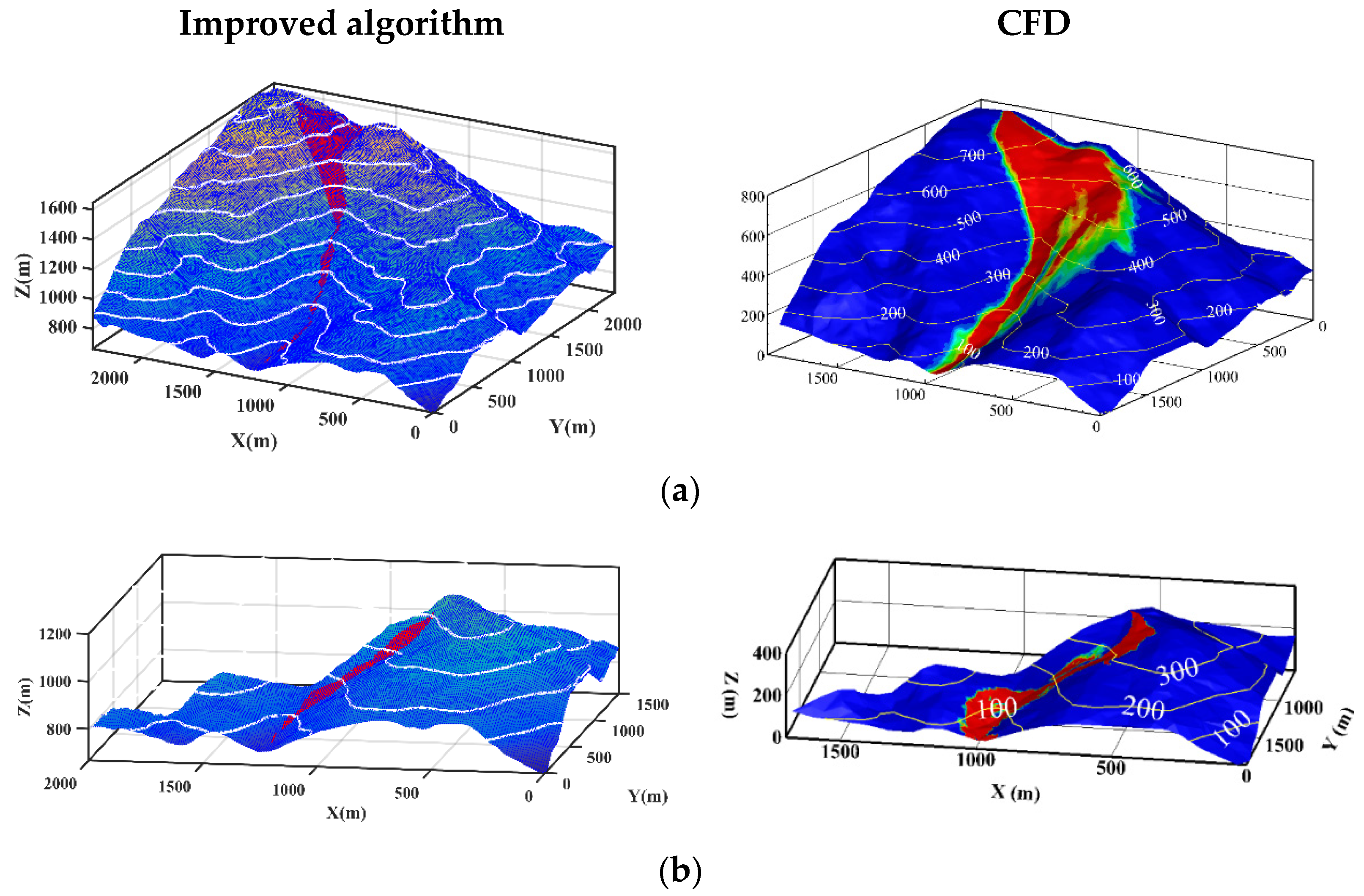
3.3. General Algorithm for Path Prediction

According to numerical simulation results, the diffusion pattern of the leaking oil is mainly determined by the terrain characteristics of mountains and the leakage rate. When the leakage rate is low, the leaked crude oil always flows along the valley line, which is the line that the contour protrudes to a high altitude.
Here, an algorithm for judging the flow direction of leaked oil through the elevations of the ground surface is introduced. For this algorithm shown in Figure 9, the surface topography is described by using square cells, as shown in Figure 10. Then, a cell match is selected with the initial location where the leak occurs. Oil flows from a certain cell to one of the eight surrounding cells. For every cell, there will be eight surrounding cells and oil will only have a single flow direction; thus, the algorithm is called the single-eight-flow-direction algorithm. For convenience, the single-eight-flow-direction algorithm is referred to as SFD8 in the following text. The single-eight-flow-direction (SFD8) algorithm was proposed by O’Callaghan and Mark [31]; it is one of the models that are often used in current flow-direction predictions. The core idea of SFD8 is listed as follows:
  • It assumes that the same amount of water is applied to each elevation data point.
  • It considers that all of the water at a certain point must flow to a neighbor cell with the lowest elevation so that the water volume in the whole Digital Elevation Mode (DEM) will be redistributed according to the difference of elevation.
  • The different water volume will be accumulated in each cell, and the valley points can be identified by setting the threshold value of catchment volume artificially.
In the present study, based on the SFD8 algorithm, an improved algorithm named MFD is proposed to predict the leak spread area of oil, and a new initialization method of flow accumulation matrix is introduced to develop the algorithm to predict the path of leaked oil.
Figure 9 depicts the workflow of the developed algorithm which can be divided into three parts, and each part corresponds to a fundamental matrix (filled DEM, flow direction and flow accumulation matrix). In part-A, the DEM data will undergo preliminary processing; the pits cell oil will have no flow direction, so the pits will be filled to ensure every cell can have a certain flow direction. In part-B—the step of calculating the flow direction—for the SFD8 algorithm, the oil will have only one definite direction of flow at each cell, while for the MFD algorithm, the oil will have a multi-flow direction at each cell. In part-C, the flow accumulation for oil in the calculation domain will be received; for the SFD8 algorithm, the flow accumulation will show the flow’s main path of leaked oil; for the MFD algorithm, the flow accumulation will show the spread area of leaked oil. Figure 10 illustrates the calculation process of the DEM matrix in each part.

3.3.1. Fill Pits

As a relatively complicated process, the researchers propose a variety of pits-filling algorithms [32,33,34]. In the present study, the DEM data have grid dimensions of approximately 80 × 80 cells with a horizontal and vertical resolution of 30 m, as a part of the DEM matrix has shown in Figure 10a. In order to facilitate data computation and extraction, the original DEM data are converted into ASCII type before starting. Note that some pits existing in the natural terrain inevitably have center cells that are smaller than those with the smallest elevation in the neighborhood. The existence of pits will lead to the inability to compute the water accumulation. Thus, it is necessary to fill and level the pits before computing the flow direction.

3.3.2. Compute Flow Directions

Note that one of the prerequisites for the filling of depressions or calculating the water accumulation is an accurate flow direction matrix. In the present study, the D8 method proposed by Fairfield and Leymarie [35] is employed to determine the flow direction. By scanning each cell of the DEM and calculating the relative slope between the cell and its 3 × 3 neighbor cell, the direction code indicating the steepest slope is assigned to the cell, see Figure 10b. The slope gradient of the neighboring cell is presented as follows:
G x , y ( i , j ) = N x , y ( i , j ) L x , y ( i , j ) ( i = 1 , 2 , 3 ; j = 1 , 2 , 3 )
L x , y = 2 1 2 1 1 1 2 1 2
where Gx,y is a 3 × 3 dimensional slope gradient matrix, cell(x, y) is the central cell, Nx,y is the neighboring cell of the cell(x, y) (a 3 × 3 dimensional elevation matrix) and Lx,y is the distance between the central cell and neighboring cells. The value of Lx,y(i,j) is 1 for cells in cardinal directions and 1.414 for cells in diagonal directions.
The SFD8 algorithm is able to predict the main flow path of leaked oil as the flow direction of oil is from one cell to only one surrounding cell; for the purpose of predicting the leak spread area of oil, the MFD algorithm is proposed. The MFD algorithm is derived from the SFD8; MFD is a short name of multi-flow direction, compared with SFD, which is a short name of single flow direction. The main difference between the MFD algorithm and the SFD8 algorithm is that in the SFD8 algorithm, the oil has only a single definite flow direction at each cell, while in the MFD algorithm, the oil has multiple possible flow directions at each cell, determining which cell the oil can flow from the center cell to the surrounding cell by setting the appropriate parameters.

3.3.3. Compute Flow Accumulations

After receiving the flow direction matrix, there is a need to initialize the flow accumulation matrix. The traditional SFD8 algorithm extracts the water system network by uniform rainfall in the entire DEM data. However, unlike rainfall, the leakage of pipelines occurs at a specific point in the entire DEM data. Thus, the algorithm was improved by considering only a certain amount of water to the leaked point, i.e., 100 is assigned to the cell (75, 74) in Figure 10c.
Once the spill occurs at a specific point, a certain amount of crude oil is initialized at the leakage point in the flow accumulation matrix, whereas the volume of crude oil in the rest is set to be zero. As the calculation proceeds, the volume of oil in each cell is updated according to the flow direction. Accordingly, the flow path of the leaked oil can be considered as the connections of the non-zero points in the flow accumulation matrix. Additionally, for the MFD algorithm, the calculation process is similar to the forementioned algorithm; the only difference is the flow direction—in the MFD algorithm, the oil will have multi-flow directions at each cell, and the leak spread area of oil can be considered as the gathering of non-zero points in the flow accumulation matrix.
It is worth noting that under the computational conditions, the computation time drops from one week taken by CFD to one minute taken by the improved algorithm. Figure 11 shows the spread area of the leaked oil, which is overlaid on the DEM. For the leakage that occurs in the valley, it can be seen that the spread area calculated by the improved algorithm is clearly thinner than the spread area calculated by the CFD method. The reason for this development is that the oil will only flow from high to low in the improved algorithm, but in the real situation, the oil will move to a higher position beside the main ditch because of its inertia velocity. Although the size of the leak spread area shows a huge difference, the general trend of the two spread areas is the same. For the leakage at the ridge, the spread area calculated by the improved algorithm and by the CFD method are more similar; by counting the red pixels, the spread area calculated by the improved algorithm is about 131 thousand square meters, and the spread area calculated by the improved algorithm is about 139 thousand square meters. The two calculation results fit well.
Compared with the CFD results, it can be inferred that the algorithm developed in the present study accurately predicts the main area of oil spread, providing a time-saving and efficient method for leakage analysis. It must be admitted that the current algorithm is only suitable for a spill at a lower rate. When the spill rate is high, the effect of gravity on the dispersion path will be reduced and the direction and magnitude of the velocity will determine the direction of dispersion of the spilled oil during the initial stages of the spill.

4. Conclusions

In this paper, the path and diffusion of leaked crude oil in a mountainous area are numerically analyzed. The effects of the leak velocity, surface conditions and terrain features have been investigated carefully. The results indicate that the terrain features affect the path of the leaked oil more prominently in comparison to the effect of the leak velocity and surface conditions. The leaked oil has the characteristic of spreading over the ridge and converging in the valley. Additionally, the diffusion area is intimately linked to the leak velocity and surface conditions. The diffusion area decreases with the increase in leak velocity. On the contrary, the diffusion area increases with increasing surface roughness. However, this enlargement effect apparently becomes less pronounced when the roughness height is greater than the average impact height of the crude oil. Based on the simulation results, a developed algorithm for predicting the path and spread area of the leaked crude oil is proposed in this paper. Although the current algorithm is only suitable for a spill at a lower rate, it provides a new approach to predict the path of fluid flow in complex mountainous environments.

Author Contributions

Conceptualization, K.W.; methodology, K.W. and J.P.; software, J.P. and B.H.; validation, J.P., J.Z. and B.H.; formal analysis, K.W. and J.Z.; investigation, J.Z.; resources, K.W. and J.P.; data curation, J.Z.; writing—original draft preparation, K.W. and J.Z.; writing—review and editing, K.W. and J.P.; visualization, B.H.; supervision, K.W.; project administration, K.W.; funding acquisition, K.W. All authors have read and agreed to the published version of the manuscript.

Funding

The research was supported by the National Natural Science Foundation of China (Grant No. 51706245), the Science Foundation of China University of Petroleum, Beijing (Grant No. 2462016YJRC029, 2462020YX22042) and the Strategic Cooperation Technology Projects of CNPC and CUPB (Grant No. ZLZX2020-05).

Informed Consent Statement

Not applicable.

Conflicts of Interest

The authors declare no conflict of interest.

Nomenclature

ρoildensity of crude oil, M/L3 kg/m3
ρairdensity of air, M/L3, kg/m3
μoilviscosity of crude oil, M/L·t, kg/m·s
μairviscosity of air, M/L·t, kg/m·s
z0roughness length, L, m
KSRoughness height, L, m
ttime of crude oil leakage, t, s
vinitial leakage velocity, L/t, m/s
Gx,y3 × 3 dimensional slope gradient matrix
Nx,yneighboring cell of the cell (x, y)
Lx,ydistance between central cell and neighboring cells

References

  1. Liang, S. China-myanmar energy pipelines important for their geo-strategic position. China Oil Gas 2013, 2, 13–15. [Google Scholar]
  2. Mitra-Thakur, S. China receives first natural gas from Myanmar pipeline. Eng. Technol. 2013, 8, 16. [Google Scholar]
  3. Anonymous. CNPC to build and operate China-Myanmar pipeline. Pipeline Gas J. 2010, 237, 14. [Google Scholar]
  4. Di, B.F.; Chen, N.S.; Cui, P.; Li, Z.L.; He, Y.P.; Gao, Y.C. GIS-based risk analysis of debris flow: An application in Sichuan, southwest China. Int. J. Sediment Res. 2008, 2, 138–148. [Google Scholar] [CrossRef]
  5. Anbalagan, R.; Singh, B. Landslide hazard and risk assessment mapping of mountainous terrains-a case study from Kumaun Himalaya, India. Eng. Geol. 1996, 43, 237–246. [Google Scholar] [CrossRef]
  6. Ciriello, V.; Lauriola, I.; Bonvicini, S.; Cozzani, V.; Di Federico, V.; Tartakovsky, D.M. Impact of hydrogeological uncertainty on estimation of environmental risks posed by hydrocarbon transportation networks. Water Resour. Res. 2017, 53, 8686–8697. [Google Scholar] [CrossRef]
  7. Briscoe, F.; Shaw, P. Spread and evaporation of liquid. Pergamon 1980, 6, 127–140. [Google Scholar] [CrossRef]
  8. Fay, J.A. The Spread of Oil Slicks on a Calm Sea; Springer: Boston, MA, USA, 1969; pp. 53–63. [Google Scholar]
  9. Kapias, T.; Griffiths, R.F. Accidental releases of titanium tetrachloride (TiCl4) in the context of major hazards-spill behaviour using reactpool. J. Hazard. Mater. 2005, 119, 41–52. [Google Scholar]
  10. Kapias, T.; Griffiths, R.F.; Stefanidis, C. Spill behaviour using reactpool: Part II. Results for accidental releases of silicon tetrachloride (SiCl(4)). J. Hazard. Mater. 2001, 81, 209–222. [Google Scholar]
  11. Kapias, T.; Griffiths, R.F. Spill behaviour using reactpool: Part III. Results for accidental releases of phosphorus trichloride (PCl(3)) and oxychloride (POCl(3)) and general discussion. J. Hazard. Mater. 2001, 81, 223–249. [Google Scholar] [CrossRef]
  12. Webber, D.M. On models of spreading pools. J. Loss Prev. Process Ind. 2012, 25, 923–926. [Google Scholar] [CrossRef]
  13. Witlox, H.W.M.; Maria, F.; Mike, H.; Oke, A.; Stene, J.; Xu, Y. Verification and validation of phast consequence models for accidental releases of toxic or flammable chemicals to the atmosphere. J. Loss Prev. Process Ind. 2018, 55, 457–470. [Google Scholar] [CrossRef]
  14. Wu, G.Z.; Guo, E.Y.; Qi, H.B.; Zhou, Y.M.; Li, D. The Impact Analysis on Crude Oil Phase Change to the Migration of Buried Oil Pipelines Leakage Pollution. Appl. Mech. Mater. 2014, 3547, 675–677. [Google Scholar]
  15. Ji, X.Y.; Liu, X.Y. Soil Columns’ Experiments by Layers of the Migration of Petroleum Hydrocarbons Contaminants in Soils. Energy Environ. Prot. 2005, 19, 43–45. [Google Scholar]
  16. He, G.; Lyu, X.; Liao, K.; Li, Y.; Sun, L. A method for fast simulating the liquid seepage-diffusion process coupled with internal flow after leaking from buried pipelines. J. Clean. Prod. 2019, 240, 118167. [Google Scholar] [CrossRef]
  17. Norouzi, S.; Soleimani, R.; Farahani, M.V.; Rasaei, M.R. Pore-Scale Simulation of Capillary Force Effect in Water-Oil Immiscible Displacement Process in Porous Media. In Proceedings of the 81st EAGE Conference and Exhibition, London, UK, 3–6 June 2019; European Association of Geoscientists & Engineers: Houten, The Netherlands, 2019. [Google Scholar]
  18. Cavanaugh, T.A.; Siegell, J.H.; Steinberg, K.W. Simulation of vapor emissions from liquid spills. J. Hazard. Mater. 1994, 38, 41–63. [Google Scholar] [CrossRef]
  19. Tauseef, S.M.; Pandey, S.K.; Abbasi, T.; Abbasi, S.A. An Assessment of the Spread Rates of Accidentally Spilled Flammable Liquids and the Development of a Model to Forecast the Spill Velocity. J. Fail. Anal. Prev. 2019, 19, 1774–1780. [Google Scholar] [CrossRef]
  20. Benfer, M. Spill and Burning Behavior of Flammable Liquids. Ph.D. Thesis, University of Maryland, College Park, MD, USA, 2010. [Google Scholar]
  21. Raja, S.; Reddy, T.; Tauseef, S.M.; Abbasi, T.; Abbasi, S.A. Efficacy of existing transient models for spill area forecasting. J. Chem. Health Saf. 2019, 26, 33–37. [Google Scholar]
  22. Hussein, M.; Jin, M.; Weaver, J.W. Development and verification of a screening model for surface spreading of petroleum. J. Contam. Hydrol. 2002, 57, 281–302. [Google Scholar] [CrossRef]
  23. Blokker, P.C. Spreading and evaporation of petroleum products on water. In Proceedings of the 4th International Har-Bour Conference, Antwerp, Belgium, 22–27 June 1964; pp. 911–919. [Google Scholar]
  24. Al-Rabeh, A.H.; Cekirge, H.M.; Gunay, N. A stochastic simulation model of oil spill fate and transport. Appl. Math. Model. 1989, 13, 322–329. [Google Scholar] [CrossRef]
  25. Karafyllidis, I. A model for the prediction of oil slick movement and spreading using cellular automata. Environ. Int. 1997, 23, 839–850. [Google Scholar] [CrossRef]
  26. Lehr, W.J.; Overstreet, R. ADIOS-Automated Data Inquiry for oil spills. In Proceedings of the Fifteenth Arctic and Marine oil Spill Program Technical Seminar, Edmonton, AB, Canada, 10–12 June 1992; pp. 31–45. [Google Scholar]
  27. Geng, X.; De Boufa, L.M.C.; Ozgokmen, T.; King, T.; Lee, K.; Lu, Y.; Zhao, L. Oil droplets transport due to irregular waves: Development of large-scale spreading coefficients. Mar. Pollut. Bull. 2016, 104, 279–289. [Google Scholar] [CrossRef] [PubMed]
  28. Zheng, Y.P.; Yang, R.; Wang, R.; Yao, H. A new modelling method of CFD real terrain based on contour lines. Yangtze River 2017, 48, 40–45. [Google Scholar]
  29. Ti, Z.L.; Li, Y.L.; Liao, H.L. Effect of ground surface roughness on wind field over bridge site with a gorge in mountainous area. Eng. Mech. 2017, 34, 73–81. [Google Scholar]
  30. Hirt, C.W.; Nichols, B.D. Volume of fluid (VOF) method for the dynamics of free boundaries. Acad. Press 1981, 39, 201–225. [Google Scholar] [CrossRef]
  31. O’Callaghan, J.F.; Mark, D.M. The extraction of drainage networks from digital elevation data. Comput. Vis. Graph. Image Process. 1984, 28, 323–344. [Google Scholar] [CrossRef]
  32. Martz, L.W.; Jong, E.D. Catch: A fortran program for measuring catchment area from digital elevation models. Comput. Geosci. 1988, 14, 627–640. [Google Scholar] [CrossRef]
  33. Barnes, R.; Lehman, C.; Mulla, D. Priority-flood: An optimal depression-filling and watershed-labeling algorithm for digital elevation model. Comput. Geosci. 2014, 62, 117–127. [Google Scholar] [CrossRef] [Green Version]
  34. Cheng, S.; Xi, Z.W.; Cun, J.F.; Huang, Z.; Zhang, X. An integrated algorithm for depression filling and assignment of drainage directions over flat surfaces in digital elevation model. Earth Sci. Inform. 2015, 8, 895–905. [Google Scholar]
  35. Fairchild, J.; Leymarie, P. Drainage networks from grid digital elevation models. Water Resour. Res. 1991, 27, 709–717. [Google Scholar]
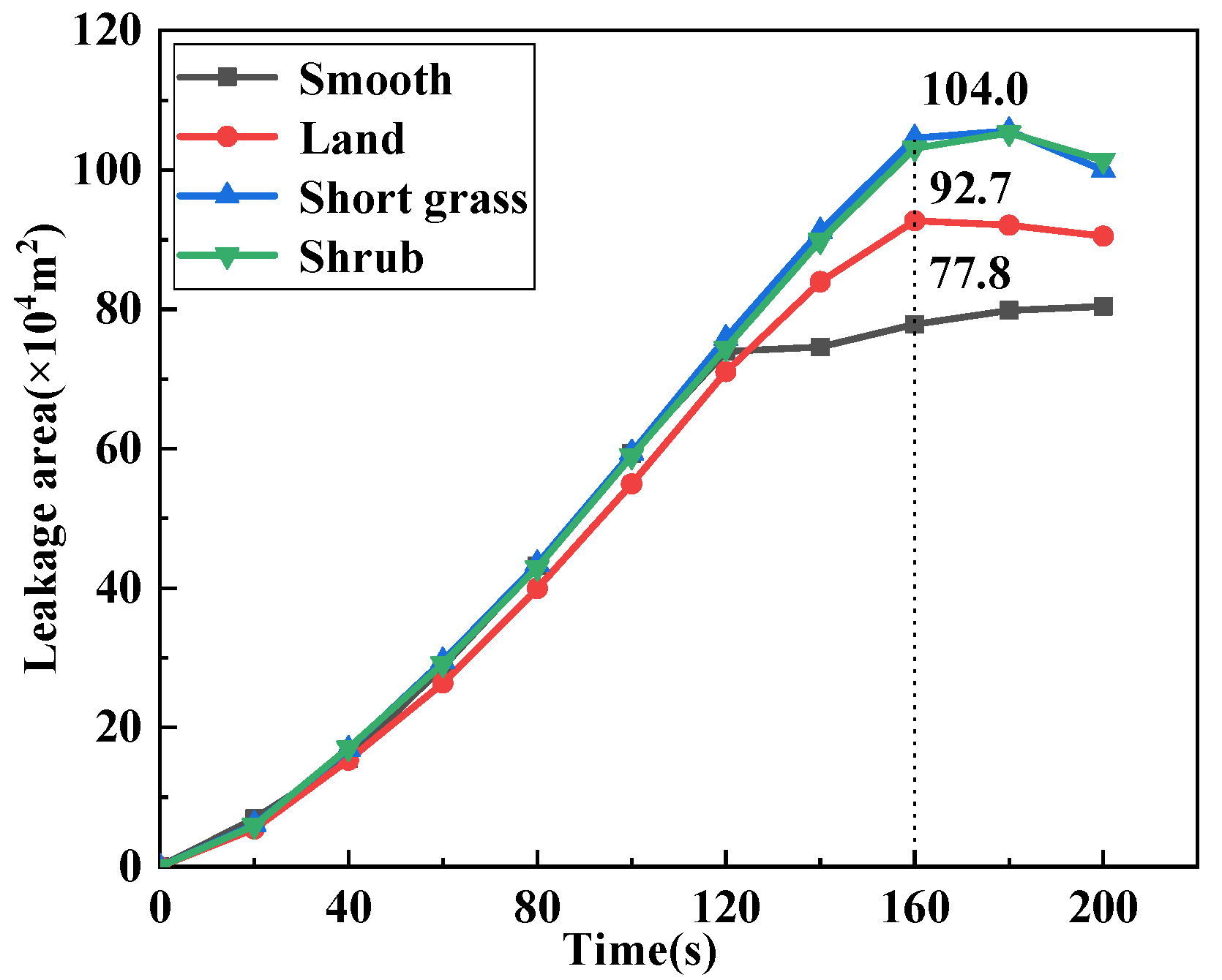
Figure 1. Terrain extraction: (a) Terrain elevation data; (b) Contour lines; (c) Extracted terrain surface; (d) Computational domain.
Energies 15 06568 g001
Figure 2. Grid details.
Energies 15 06568 g002
Figure 3. Crude oil diffusion patterns on smooth surface: (a) v =30 m/s; (b) v = 50 m/s; (c) v = 80 m/s.
Energies 15 06568 g003aEnergies 15 06568 g003bEnergies 15 06568 g003c
Figure 4. Trend of the crude oil leakage area at different leak velocities.
Energies 15 06568 g004
Figure 5. Diffusion patterns of leaked crude oil on different mountain surfaces: (a) Rough land; (b) Short grass/s; (c) Shrub.
Energies 15 06568 g005aEnergies 15 06568 g005b
Figure 6. Trend of the crude oil leakage area on different surfaces.
Energies 15 06568 g006
Figure 7. Diffusion patterns of the leaked crude oil when the leakage occurs at the ridge: (a) v = 30 m/s; (b) v = 50 m/s; (c) v = 80 m/s.
Energies 15 06568 g007aEnergies 15 06568 g007bEnergies 15 06568 g007c
Figure 8. Variation of the diffusion area at different leak velocities.
Energies 15 06568 g008
Figure 9. Workflow of the oil-leaking simulation based on the SFD algorithm.
Energies 15 06568 g009
Figure 10. Matrix calculus process, the cell in red color means the cell is a part of leak spread area, the cell in grey means the cell is a pit, and the cell in white means it’s a normal cell: (a) Filling pits; (b) Flow direction; (c) Flow accumulation.
Energies 15 06568 g010
Figure 11. Comparison between the improved algorithm with CFD (v = 30 m/s): (a) Leakage in the valley; (b) Leakage at the ridge.
Energies 15 06568 g011
Table 1. Roughness of different surface conditions.
Surface Type Roughness   Length   z 0 / m Roughness   Height   K s / m
Smooth land00
Rough land0.0250.5
Short grass0.12
Shrub0.24
Publisher’s Note: MDPI stays neutral with regard to jurisdictional claims in published maps and institutional affiliations.

