Multi-Objective Optimization via GA Based on Micro Laser Line Scanning Data for Micro-Scale Surface Modeling

Abstract

Industry 4.0 represents high-level methodologies to make intelligent, autonomous, and self-adaptable manufacturing systems. Additionally, the surface modeling technology has become a great tool in industry 4.0 for representing the surface point cloud. Thus, the micro-scale machining technology requires efficient models to represent micro-scale flat and free-form surfaces. Therefore, it is fundamental to perform surface modeling through artificial intelligence for representing small surfaces. This study addressed multi-objective optimization via genetic algorithms and micro laser line projection to accomplish surface models for representing micro-scale flat and free-form surfaces, where an optical microscope system retrieves micro-scale topography via micro laser line coordinates and the multi-objective optimization constructs the flat and free-form surface models through genetic algorithms and micro-scale topography. The multi-objective optimization determines the surface model parameters through exploration and exploitation, and the solution space is deduced via surface data. The surface model generated through the multi-objective optimization fit accurately to the micro-scale target surface. Thus, the proposed technique enhanced the fitting of micro-scale flat and free-form surface models, which were deduced via gray-level images of an optical microscope. This enhancement was validated by a discussion between the multi-objective optimization via genetic algorithms and the micro-scale surface modeling via optical microscope imaging systems.

1. Introduction

Nowadays, the manufacturing industry is developing intelligent tools to accomplish the requirements of industry 4.0. The intelligent tools include cyber-physical systems, Internet of Things, information technology, digital manufacturing activities, and so on [1]. The cyber-physical systems are involved in the manufacturing systems based on artificial intelligence and the self-adaptable process [2]. However, the Internet of Things provides tools to store and share the surface point cloud in the manufacturing systems during the production process [3]. In this way, the cyber-physical systems, Internet of Things, digital manufacturing, and information technology determine the surface point cloud and perform surface modeling to represent a small object surface in digital form. Additionally, the surface modeling provides fundamental tools in industry 4.0 to represent computationally flat and free-form surfaces [4,5]. In the same way, the flat and free-form surface modeling at the micro-scale provides computational tools in industry 4.0 to represent micro-scale objects [6,7], where the computational tools are constructed via mathematical models to generate flat and free-form surfaces at the micro-scale. Actually, micro-scale flat and free-form surface modeling is performed via optical microscope systems based on gray-level image processing in industry 4.0 [8,9]. The microscope systems perform surface recovering and mathematical modeling to accomplish micro-scale surface modeling. Typically, the micro-scale surface modeling is accomplished through the least-squares method, and the surface data are determined via optical microscope images [10,11]. However, the surface fitting of the least-squares method produced inaccuracy with respect to the target surface [12]. Therefore, artificial intelligence methods have been implemented to perform micro-scale surface modeling in industry 4.0. For instance, the particle swarm has been implemented to perform free-form surface modeling through equations based on particle movement [13,14], where the parameter optimization has been carried out through a population generated by means of particle velocity. Additionally, particle swarm optimization has been employed in several optimization applications to achieve a good fit and convergence [15,16]. However, the particle swarm is a metaheuristic algorithm more employed to optimize surface modeling. Additionally, ant colony has been implemented to perform free-form surface modeling in industry 4.0 [17,18], where the parameter optimization has been carried out by selecting pathways generated by the ant pheromone to accomplish the computational model. In the same way, simulated annealing has been implemented to construct free-form surface models in industry 4.0 [19,20], where the model parameters have been computed through a perturbation in an equation system. Additionally, fuzzy logic has been implemented to generate free-form surface models in industry 4.0 [21,22], where the model parameters have been optimized by using contactless scanning of the transtibial prosthetic socket. Furthermore, virtual reality was implemented to perform free-form surface models through a spline function [23], where a convex approximation was carried out through the spline basis function to determine concave surface models. Moreover, machine learning was implemented to perform flat surface models via neural networks [24], where the flat surface equation was constructed from the topography contour data. On the other hand, the micro-scale surface models are constructed through surface data, which are determined by means of optical microscope images. For example, a microscope imaging system determined free-form surfaces at the micro-scale by computing data through the optical microscope images [25]. Additionally, a microscope imaging system performed flat contouring at the micro-scale by computing surface data through the optical microscope images [26], where a frequency transform was computed from the gray-level image to determine the surface data. Moreover, a microscope imaging system retrieved flat topography at the micro-scale through a regression model and optical microscope images [27], where a fitting function was generated by means of the gray-level image to determine the surface data. The above microscope arrangements perform the surface modeling at the micro-scale through the surface data, which are determined by means of optical microscope images. However, the gray-level profile does not depict the topography contour with the best accuracy. The profile inaccuracy is caused by the object reflectance, light transmitter source, and viewer direction. Therefore, the computational model produces flat and free-form surfaces away from the target surface. In addition, the above-mentioned methods optimize the surface model parameters through a search space, which is not deduced from the surface data. For instance, the free-form surface models generated through the simulated annealing, particle swarm, and ant colony are not accomplished by means of surface data. Such algorithms determine the model parameters through a solution space, which is not deduced from the surface topography. As a consequence of missing references, complicated procedures should be implemented to optimize the model parameters. Moreover, the minimization function is deduced through a mathematical expression, which includes additional variables to the surface model. Therefore, the additional variables should be computed to optimize the surface model parameters. Although the flat and free-form surface modeling at the micro-scale represents one of the central paradigms of industry 4.0, it still requires further research and development. Therefore, it is established that the flat and free-form surface modeling performed at the micro-scale via optical microscope systems still represents a difficult challenge. To enhance the flat and free-form surface modeling at the micro-scale, a multi-objective optimization based on several objective functions and surface contour data is required. It is because the free-form surface is generated through several surface functions. The multi-objective optimization via genetic algorithms was implemented in several applications [28] and provided good fitting and convergence results.

The proposed flat and free-form surface modeling at the micro-scale is performed through multi-objective optimization and micro laser line scanning, which retrieves surface contour with great accuracy. The multi-objective optimization is implemented through a genetic algorithm, which employs several objective functions to construct micro-scale flat and free-form surface models. In this way, the free-form surface modeling is implemented through objective functions, which are generated through the Bezier basis functions and surface control points. Additionally, the flat surface modeling is implemented through objective functions, which are generated through the plane equation and surface data. Thus, the genetic algorithm performs micro-scale flat and free-form surface modeling by employing surface coordinates, which are computed from the laser line coordinates. To carry it out, the multi-objective optimization determines the solution space from the surface coordinates. Then, exploration and exploitation are performed to determine the optimal model parameters from the solution space. The main approach to perform flat and free-form surface modeling through genetic algorithms is determined by the quality gap, number of iterations, and suitable structure. For instance, the particle swarm, ant colony, and simulated annealing do not determine the solution space through the surface data. Instead, the genetic algorithm determines the solution space from the surface data. This leads to obtaining an initial population near of the optimal solution and reduces the number of iterations. Furthermore, the other intelligent algorithms employ additional parameters to the surface model and increase the number of iterations. Additionally, the genetic algorithm provides a better surface model fitting than the other intelligent algorithms. Moreover, the genetic algorithm performs exploration and exploitation to find the optimal solution inside or outside of the best candidates. Based on these statements, the genetic algorithm was chosen to perform the flat and free-form surface models. In this way, the micro-scale flat and free-form surface modeling was performed by an optical microscope vision system on which a CCD camera and a 38 μm laser line were attached. Thus, the micro laser line was projected on the surface and the reflection depicted the surface contour, which was captured by the CCD camera. The micro-scale surface coordinates were computed through the microscope geometry and the laser line position. Thus, the micro-scale flat and free-form surface models were accomplished through the surface coordinates, which are not used by the optical microscope systems. Therefore, the micro-scale flat and free-form surface modeling via multi-objective optimization and the micro laser line scanning enhanced the surface model fitting of the optical microscope systems, where the fitting accuracy was deduced through the difference between the data computed through the surface model and the real surface data. The multi-objective optimization was employed to construct micro-scale models of rectangular surfaces. The viability of the multi-objective optimization via genetic algorithms was deduced through the model fitting, run time, algorithm structure, and results’ accuracy. To corroborate this statement, a discussion is provided about the fitting accuracy of the surface models at the micro-scale. In this way, the viability of the proposed technique is corroborated by the fitting accuracy of the micro-scale flat and free-form surface modeling. The paper is organized as follows: the multi-objective optimization to construct the free-form surface model at the micro-scale is explained in Section 2.1, the multi-objective optimization to construct the flat surface model at the micro-scale is explained in Section 2.2, the surface contouring at the micro-scale through the microscope vision system is described in Section 2.3, the results of the flat and free-form surface modeling at the micro-scale are shown in Section 3, and the model fitting discussion is included in Section 4.

2. Materials and Methods

2.1. Multi-Objective Optimization for Micro-Scale Free-Form Surface Modeling

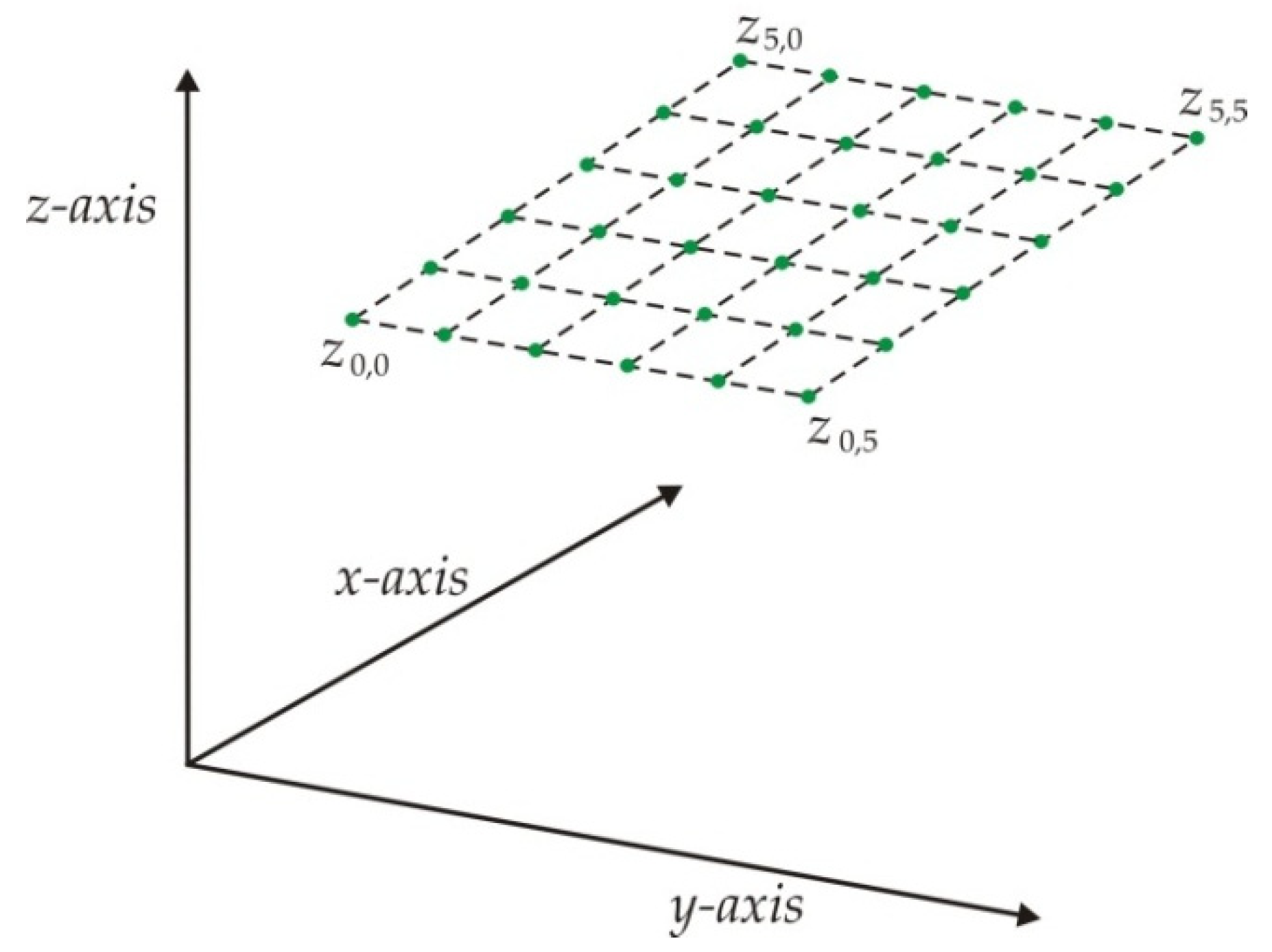
The free-form surface modeling at the micro-scale is performed through the multi-objective optimization and surface coordinates, which are computed via laser line scanning. Typically, the multi-objective optimization employs several objective functions to be minimized and guarantees to find the ideal solution [29]. In this way, the multi-objective optimization operates on a set of solution spaces and employs a moderated time to achieve the optimization. Additionally, exploration and exploitation are implemented by the multi-objective optimization to determine the optimal solution from the solution space. Thus, the free-form surface modeling at the micro-scale is carried out through the multi-objective optimization based on a genetic algorithm and the contour data. To do so, the free-form surface is retrieved via micro laser line scanning. The contour coordinates are shown in Figure 1, and they are represented by (x_i,j, y_i,j, z_i,j), where the sub-indices (i, j) are established in the x-axis and y-axis, respectively. In this way, the surface provides the coordinates (z_0,0, z_1,0, …, z_n,0, z_n,1, …, z_n,m) in the z-axis, where the sub-indices (n, m) depict the coordinate number in the x-axis and y-axis, respectively.

From the surface coordinates, the free-form surface model is constructed through a bi-cubic Bezier surface [30], which is described by the expression

$$\begin{array}{c}{S}_{p,q}(u,v)={\displaystyle \sum _{s=0}^{s=3}{\displaystyle \sum _{r=0}^{r=3}{B}_r(u)B_s}(v)}{P}_{i,j},\hspace{1em}\hspace{1em}u,v\in [0,1],\\ B_r(u)=\frac{3!}{r!(3-r)!}{(1-u)}^{3-r}{u}^r,\hspace{1em}\hspace{1em}{B}_s(v)=\frac{3!}{s!(3-s)!}{(1-v)}^{3-s}{v}^s.\end{array}$$

(1)

In this equation, u is in the x-direction, v is in the y-direction, and P_i,j are control points that move the Bezier surface toward the surface z_i,j. The sub-indices (i, j) are related to the sub-indices (r, s) through the terms i = r + p*3 and j = s + q*3, respectively. In this way, the free-form surface model is represented by the surfaces S_0,0(u,v), S_1,0(u,v), …, S_n/3,0(u,v), …, S_n/3,m/3(u,v). Thus, the free-form surface model is defined by the equation

$$\left[\begin{array}{l}{S}_{0,0}(u,v)\\ \\ \\ S_{1,0}(u,v)\\ \\ \\ S_{0,1}(u,v)\\ \\ ⋮\\ S_{n/3,m/3}(u,v)\\ \end{array}\right]=\left[\begin{array}{l}{B}_{0,0}{P}_{0,0}+B_{1,0}{P}_{1,0}+B_{2,0}{P}_{2,0}+B_{3,0}{P}_{3,0}+B_{0,1}{P}_{0,1}+B_{1,1}{P}_{1,1}+B_{2,1}{P}_{2,1}+B_{3,1}{P}_{3,1}+\\ B_{0,2}{P}_{0,2}+B_{1,2}{P}_{1,2}+B_{2,2}{P}_{2,2}+B_{3,2}{P}_{3,2}+B_{0,3}{P}_{0,3}+B_{1,3}{P}_{1,3}+B_{2,3}{P}_{2,3}+B_{3,3}{P}_{3,3}\\ \\ B_{0,0}{P}_{3,0}+B_{1,0}{P}_{4,0}+B_{2,0}{P}_{5,0}+B_{3,0}{P}_{6,0}+B_{0,1}{P}_{3,1}+B_{1,1}{P}_{4,1}+B_{2,1}{P}_{5,1}+B_{3,1}{P}_{6,1}+\\ B_{0,2}{P}_{3,2}+B_{1,2}{P}_{4,2}+B_{2,2}{P}_{5,2}+B_{3,2}{P}_{6,2}+B_{0,3}{P}_{3,3}+B_{1,3}{P}_{4,3}+B_{2,3}{P}_{5,3}+B_{3,3}{P}_{6,3}\\ \\ B_{0,0}{P}_{0,3}+B_{1,0}{P}_{1,3}+B_{2,0}{P}_{2,3}+B_{3,0}{P}_{3,3}+B_{0,1}{P}_{0,4}+B_{1,1}{P}_{1,4}+B_{2,1}{P}_{2,4}+B_{3,1}{P}_{3,4}+\\ B_{0,2}{P}_{0,5}+B_{1,2}{P}_{1,5}+B_{2,2}{P}_{2,5}+B_{3,2}{P}_{3,5}+B_{0,3}{P}_{0,6}+B_{1,3}{P}_{1,6}+B_{2,3}{P}_{2,6}+B_{3,3}{P}_{3,6}\\ ⋮ ⋮\\ B_{0,0}{P}_{n-3,m-3}+B_{1,0}{P}_{n-2,m-3}+B_{2,0}{P}_{n-1,m-3}+B_{3,0}{P}_{n,m-3}+B_{0,1}{P}_{n-3,m-2}+B_{1,1}{P}_{n-2,m-2}+\\ B_{2,1}{P}_{n-1,m-2}+B_{3,1}{P}_{n,m-2}+B_{0,2}{P}_{n-3,m-1}+B_{1,2}{P}_{n-2,m-1}+B_{2,2}{P}_{n-1,m-1}+B_{3,2}{P}_{n,m-1}+\\ B_{0,3}{P}_{n-3,m}+B_{1,3}{P}_{n-2,m}+B_{2,3}{P}_{n-1,m}+B_{3,3}{P}_{\begin{array}{l}n,m\\ \end{array}}\end{array}\right].$$

(2)

In this equation, B_r,s = B_r(u)B_s(v) and the control points P_i,j should be computed to determine the free-form surface model. Thus, the control points are determined by the expression P_i,j = z_i,j w_i,j, where the weights w_i,j are in the interval [0.7, 1.3]. Additionally, the initial Bezier surface Equation (1) is determined by means of w_i,j = 1, which provides the control points P_i,j = z_i,j. Additionally, the surface points are represented by the coordinates (x_i,j, y_i,j, z_i,j). Thus, the values (u, v) are computed by the expressions u = (x_3+p*3,q − x_0+p*3,q)/3 and v = (y_p,3+q*3 − y_p,0+q*3)/3, respectively. Based on these statements, the control points P_i,j are determined by means of the weights w_i,j. In this way, a multi-objective optimization through a genetic algorithm is implemented to determine the weights w_i,j. To do so, the genetic algorithm is implemented as follows.

The first step is to compute the solution space and the initial population. Typically, the multi-objective optimization based on a genetic algorithm determines the solution space through the Pareto solution method [31], where the solution space is determined from the edge between the minimum of the objective functions, which is called Pareto front [32]. However, it is necessary to establish additional criteria to determine the best solution from the line or curve of the Pareto front. This leads to implementing additional procedures in the genetic algorithm. Additionally, the multi-objective optimization based on intelligent algorithms determined the solution space through the maximum and minimum [33]. Therefore, the proposed technique determines the solution space through the initial Bezier surface, which provides the maximum or minimum of each control P_i,j. In this way, the initial Bezier surface is computed via Equation (1) by employing w_i,j = 1_j. Thus, if S_p,q(u,v) is over the surface point z_i,j, the maximum is defined as z_i,j*1.0 and the minimum is defined by z_i,j*0.7, which moves the Bezier surface under the z_i,j. On the other hand, if S_p,q(u,v) is under the surface point z_i,j, the minimum is established as z_i,j*1.0 and the maximum is defined by z_i,j*1.3, which moves the Bezier surface over the z_i,j. Thus, the solution space is generated. In this way, the initial Bezier surface provides the solution space from the surface data to perform the multi-objective optimization. Then, the initial population is generated from the solution space. To carry it out, four values are randomly computed from the solution space for each weight. These values represent the parents ($\mathcal{P}$_1,k, $\mathcal{P}$_2,k), ($\mathcal{P}$_3,k, $\mathcal{P}$_4,k), where the k-index indicates the generation number. With these parents, the initial population is completed.

The second step is to perform the crossover to create the current children. The crossover performs exploration and exploitation to create two children inside the parents and two children outside the parents [34]. In this way, the children (C_1+4*t,k, C_2+4*t,k, C_3+4*t,k, C_4+4*t,k) are created through the parents ($\mathcal{P}$_1+2*t,k, $\mathcal{P}$_2+2*t,k) for t = 0 and t = 1. Thus, the children are computed by the expressions

$$C_{1+4*t,k}=\{\begin{array}{l}{\mathcal{P}}_{1+2*t,k}-0.5\beta \left|{\mathcal{P}}_{1+2*t,k}-\mathrm{minimum}\right|,\hspace{1em}\hspace{1em}\mathrm{if}\hspace{1em}{\mathcal{P}}_{1+2*t,k}<{\mathcal{P}}_{2+2*t,k}\\ \\ {\mathcal{P}}_{2+2*t,k}-0.5\beta \left|{\mathcal{P}}_{2+2*t,k}-\mathrm{minimum}\right|,\hspace{1em}\hspace{1em}\mathrm{if}\hspace{1em}{\mathcal{P}}_{2+2*t,k}<{\mathcal{P}}_{1+2*t,k}\end{array},$$

(3)

$$C_{2+4*t,k}=0.5\left[\left(P_{1+2*t,k}+P_{2+2*t,k}\right)-\beta \left|P_{1+2*t,k}-P_{2+2*t,k}\right|\right],$$

(4)

$$C_{3+4*t,k}=0.5\left[\left(P_{1+2*t,k}+P_{2+2*t,k}\right)+\beta \left|P_{1+2*t,k}-P_{2+2*t,k}\right|\right],$$

(5)

$$C_{4+4*t,k}=\{\begin{array}{l}{P}_{2+2*t,k}+0.5\beta \left|\mathrm{maximum}-P_{2+2*t,k}\right|,\hspace{1em}\hspace{1em}\mathrm{if}\hspace{1em}{P}_{1+2*t,k}<P_{2+2*t,k}\\ \\ P_{1+2*t,k}+0.5\beta \left|\mathrm{maximum}-P_{1+2*t,k}\right|,\hspace{1em}\hspace{1em}\mathrm{if}\hspace{1em}{P}_{2+2*t,k}<P_{1+2*t,k}\end{array}.$$

(6)

In these equations, the probability distribution β is determined through the spread factor α, which is randomly computed in the interval [0, 1]. Thus, the probability distribution is β = (2α)^1/2 if α > 0.5; otherwise, β = [2(1 − α)]^1/2. In this way, the children inside the parents are computed by Equations (4) and (5), and the children outside the parents are computed by Equation (3) through Equation (6). Thus, the children (C_1,k, C_2,k, C_3,k, C_4,k) are computed by Equation (3) through Equation (6) through the parents ($\mathcal{P}$_1,k, $\mathcal{P}$_2,k) and t = 0. Then, the children (C_5,k, C_6,k, C_7,k, C_8,k) are computed by Equation (3) through Equation (6) through the parents ($\mathcal{P}$_3,k, $\mathcal{P}$_4,k) and t = 1. Thus, the current children are obtained. To assemble the Bezier surfaces S_p,q(u,v) with G¹ continuity, the boundary control points must be collinear [35]. Therefore, the boundary control points are computed by the expressions P_3+3*p,j = (P_3+3*p−1,j + P_3+3*p+1,j)/2 and P_i,3+3*q = (P_i,3+3*q−1 + P_i,3+3*q+1)/2.

The third step is to evaluate the fitness through a multi-objective function, which is deduced by the Bezier surfaces S_0,0(u,v), S_1,0(u,v), …, S_n/3,m/3(u,v). Thus, the multi-objective function is defined by the expression

$$\left[\begin{array}{l}{F}_{0,0}\\ \\ \\ F_{1,0}\\ \\ \\ F_{0,1}\\ \\ ⋮\\ F_{n/3,m/3}\end{array}\right]=\left[\begin{array}{l}\min \left\{\frac{1}{16}\sqrt{{\displaystyle \sum _{s=0}^{s=3}{\displaystyle \sum _{r=0}^{r=3}{\left[S_{0,0}(u,v)-z_{i,j}\right]}^2}}}\right\}\\ \\ \min \left\{\frac{1}{16}\sqrt{{\displaystyle \sum _{s=0}^{s=3}{\displaystyle \sum _{r=0}^{r=3}{\left[S_{1,0}(u,v)-z_{i,j}\right]}^2}}}\right\}\\ \\ \min \left\{\frac{1}{16}\sqrt{{\displaystyle \sum _{s=0}^{s=3}{\displaystyle \sum _{r=0}^{r=3}{\left[S_{0,1}(u,v)-z_{i,j}\right]}^2}}}\right\}\\ \begin{array}{cccc}& & & ⋮\end{array}\\ \min \left\{\frac{1}{16}\sqrt{{\displaystyle \sum _{i=0}^{i=3}{\displaystyle \sum _{j=0}^{j=3}{\left[S_{n/3,m/3}(u,v)-z_{i,j}\right]}^2}}}\right\}\end{array}\right].$$

(7)

From this multi-objective function, the fitness is computed by the expression fitness = (F_0,0 + F_1,0 + F_0,1 + …. + F_n/3,m/3)/[(n/3)(m/3)].

The fourth step is to select the parents of the next generation through the best parents and children. Thus, the parents $\mathcal{P}$_1,k+1 and $\mathcal{P}$_3,k+1 are selected from the parents ($\mathcal{P}$_1,k, $\mathcal{P}$_2,k) and ($\mathcal{P}$_3,k, $\mathcal{P}$_4,k), respectively. Then, the parents $\mathcal{P}$_2,k+1 and $\mathcal{P}$_4,k+1 are selected from the children (C_1,k, C_2,k, C_3,k, C_4,k) and (C_5,k, C_6,k, C_7,k, C_8,k), respectively.

The fifth step is to perform the mutation. This procedure leads to avoiding trapping in a local minimum. To carry it out, a new parent is randomly generated from the search space. Then, the new parent replaces the worst parent, which is selected through the fitness Equation (7). Thus, if the new parent improves the fitness, the worst parent is replaced by the new parent. Otherwise, the worst parent is not replaced. Additionally, one weight is mutated from a parent, which is selected in random form. To do so, a new weight is randomly generated from the search space, and it is replaced by the selected parent to compute the fitness Equation (7). If the new weight improves the fitness, the mutation is carried out; if not, the weight is not mutated. Thus, the mutation is accomplished to determine the parents of the (k + 1) generation. Then, the children of the (k + 1) generation are generated through the crossover by computing Equation (3) through Equation (6). From this step, the population of the (k + 1) is completed. The steps to determine the (k + 1) generation are repeated until the multi-objective function in Equation (7) is minimized.

To elucidate the multi-objective optimization, a free-form surface model was used by employing the contour data shown in Figure 2a. This procedure was performed through the flowchart shown in Figure 2b, which describes the steps to perform the free-form surface modeling via multi-objective optimization. In this way, the first step was carried out to determine the initial population. To do so, the initial Bezier surface Equation (1) was computed to define the solution space through the maximum and minimum of each control point P_i,j. In this case, control point P_0,0 was provided by the initial Bezier surface, and the data (P_3,0, P_3,1, P_3,2, P_3,3, P_0,3, P_1,3, P_2,3) were computed through the expressions P_3+3*p,j = (P_3+3*p−1,j + P_3+3*p+1,j)/2 and P_i,3+3*q = (P_i,3+3*q−1 + P_i,3+3*q+1)/2 to provide continuity G¹. Thus, the first parents were computed from the search space. The data of the initial population of the surface S_0,0(u,v) are shown in

Table 1. Control points generated in the first and second generation.

Pi,j	k	$\mathcal{P}$1	$\mathcal{P}$2	$\mathcal{P}$3	$\mathcal{P}$4	C1	C2	C3	C4	C5	C6	C7	C8
P1,0	1	4.781	4.766	4.375	4.740	4.668	4.768	4.775	4.733	4.364	4.451	4.672	4.199
P2,0	1	4.329	4.645	4.238	4.064	4.254	4.456	4.527	4.605	4.063	4.071	4.153	4.216
P0,1	1	4.753	4.144	4.550	4.698	4.131	4.175	4.514	4.737	4.458	4.623	4.695	4.501
P1,1	1	4.396	4.643	4.771	4.394	4.266	4.479	4.636	4.601	4.265	4.428	4.755	4.716
P2,1	1	4.163	4.487	4.549	4.533	4.162	4.184	4.486	4.419	4.382	4.537	4.546	4.468
P0,2	1	4.724	4.117	4.736	4.094	4.085	4.375	4.439	4.660	4.092	4.097	4.570	4.663
P1,2	1	4.318	4.543	4.657	4.484	4.215	4.382	4.450	4.514	4.457	4.512	4.643	4.633
P2,2	1	4.346	4.118	4.525	4.508	4.084	4.210	4.311	4.259	4.433	4.509	4.519	4.449
fitness		0.258	0.179	0.193	0.166	0.106	0.188	0.256	0.269	0.085	0.130	0.222	0.159
P1,0	2	4.766	4.668	4.740	4.364	4.380	4.670	4.748	4.754	4.221	4.447	4.625	4.685	4.135
P2,0	2	4.645	4.254	4.064	4.063	4.234	4.320	4.535	4.569	4.058	4.063	4.064	3.880	4.074
P0,1	2	4.144	4.131	4.698	4.458	4.104	4.133	4.143	3.803	4.303	4.459	4.587	4.683	4.154
P1,1	2	4.643	4.266	4.394	4.265	4.186	4.440	4.464	4.605	4.184	4.327	4.371	4.283	4.195
P2,1	2	4.487	4.162	4.533	4.382	4.130	4.314	4.454	4.348	4.359	4.420	4.481	4.473	3.992
P0,2	2	4.117	4.085	4.094	4.092	4.067	4.096	4.114	4.001	4.073	4.092	4.093	3.786	4.112
P1,2	2	4.059	4.215	4.484	4.457	4.028	4.071	4.178	3.935	4.395	4.457	4.481	4.421	4.163
P2,2	2	4.118	4.084	4.507	4.433	3.998	4.088	4.115	3.900	4.232	4.452	4.487	4.432	3.981
fitness		0.179	0.106	0.166	0.085	0.062	0.120	0.155	0.155	0.054	0.097	0.140	0.112	0.0126

. In this table, the first column indicates the control points, the second column indicates the generation number, and the parents ($\mathcal{P}$_1,1, $\mathcal{P}$_2,1, $\mathcal{P}$_3,1, $\mathcal{P}$_4,1) are indicated in the third to sixth column. Then, the second step was performed to compute the current children through the crossover. To carry it out, Equation (3) through Equation (6) were computed by employing the parents ($\mathcal{P}$_1+2*t,k, $\mathcal{P}$_2+2*t,k) and t = 0 to generate the children (C_1,k, C_2,k, C_3,k, C_4,k). In the same way, Equation (3) through Equation (6) were computed by employing the parents ($\mathcal{P}$_1+2*t,k, $\mathcal{P}$_2+2*t,k) and t = 1 to determine (C_5,k, C_6,k, C_7,k, C_8,k). The children data are in the seventh to fourteenth column of Table 1. Next, the third step was performed to evaluate the fitness by means of the multi-objective function, which was deduced through the Bezier surfaces S_0,0(u,v), S_1,0(u,v), …, S_1,1(u,v). This procedure indicated that the initial population produced a low error. Then, the fourth step was carried out to select the parents of the next generation from the best current parents and children. In this way, the parents $\mathcal{P}$_1,k+1 and $\mathcal{P}$_3,k+1 were selected from the pairs ($\mathcal{P}$_1,k, $\mathcal{P}$_2,k) and ($\mathcal{P}$_3,k, $\mathcal{P}$_4,k), respectively. Additionally, the parents $\mathcal{P}$_2,k+1 and $\mathcal{P}$_4,k+1 were selected from the children (C_1,k, C_2,k, C_3,k, C_4,k) and (C_5,k, C_6,k, C_7,k, C_8,k), respectively. In this case, $\mathcal{P}$_1,2 = $\mathcal{P}$_2,1, $\mathcal{P}$_3,2 = $\mathcal{P}$_4,1, $\mathcal{P}$_2,2 = C_1,1, and $\mathcal{P}$_4,2 = C_5,1. Then, the fifth step was performed to mutate the parent $\mathcal{P}$_1,2, which was selected as the worst parent. Additionally, a new parent was randomly generated from the solution space to compute the fitness (7). In this case, the fitness was not improved and the parent was not mutated. Then, the parent $\mathcal{P}$_1,2 was chosen in random form to mutate the weight w_1,2, which was randomly selected. Next, a new weight was replaced in the parent $\mathcal{P}$_1,2, and the fitness was computed via Equation (7). In this case, the fitness was improved; therefore, the weight w_1,2 was mutated. Then, the second step was carried out by computing Equation (3) through Equation (6) to create the children of the (k + 1) generation. Further, the fitness of these children was computed via Equation (7). Additionally, the control points (P_3,0, P_3,1, P_3,2, P_3,3, P_0,3, P_1,3, P_2,3) were determined by the expressions P_3+3*p,j = (P_3+3*p−1,j + P_3+3*p+1,j)/2 and P_i,3+3*q = (P_i,3+3*q−1 + P_i,3+3*q+1)/2 to provide continuity G¹.

The second-generation population is indicated in the tenth to twenty-fourth row of Table 1. In this way, the steps to compute the (k+1) generation were repeated until the multi-objective function in Equation (7) was minimized. The optimal control points are shown in the fifteenth column of Table 1. These control points define the free-form surface model, which generates the surface shown in Figure 2c. Thus, the free-form surface modeling was performed through multi-objective optimization. Additionally, this method can be performed to construct a free-form surface model for a non-rectangular surface. In this case, the contour in the x-axis and y-axis should be represented through the Bezier functions X_p,q(u,v) and Y_p,q(u,v), respectively. These functions are deduced via Equation (1) by the expressions X_p,q(u,v) = B₀(u)B₀(v)x_0,0 + B₁(u)B₀(v)x_1,0 + … + B₃(u)B₃(v)x_3,3 and Y_p,q(u,v) = B₀(u)B₀(v)y_0,0 + B₁(u)B₀(v)y_1,0 + … + B₃(u)B₃(v)y_3,3. Thus, the free-form surface model for a non-rectangular surface is defined by {X_p,q(u,v), X_p,q(u,v), S_p,q(u,v)}.

The efficiency of the multi-objective optimization is elucidated through the parameters in the genetic algorithm. The parameters include the population size, number of generations, crossover probability and mutation probability, and optimal gap. The population size indicates the number of chromosomes in one generation. In this case, each control point included an initial population of twelve chromosomes. However, each surface function S_p,q(u,v) included eight control points. Therefore, one generation included a population 384 chromosomes. The crossover probability indicates how often the crossover is performed. The crossover is made to find better chromosomes. However, it is good to leave some of the old population for the next generation. The probability of crossover is determined via fitness [36]. When the fitness average is improved, the crossover is carried out. This procedure avoids the loss of candidates to achieve the convergence. In this way, the multi-objective optimization is performed several times for the same free-form surface model. The result of the probability of crossover was in the interval from 0.18 to 0.56. The mutation probability indicates how often the chromosome can be mutated. The mutation probability is determined via fitness. In the genetic algorithm, if the fitness is improved, the mutation is carried out; if not, the parameter is not mutated. In this way, the multi-objective optimization is performed several times on the same free-form surface model. The result of the probability of mutation was in the interval from 0.26 to 0.61. The number of generations indicates the number of iterations to obtain the optimal control points. In this case, 92 generations were performed to optimize the parameters. The flat surface modeling via multi-objective optimization is described in Section 2.2. The optimal gap was computed through the relative error, and the result was 0.38%.

2.2. Micro-Scale Flat Surface Modeling via Multi-Objective Optimization

The micro-scale flat surface modeling is performed through the multi-objective optimization and surface points, which are contoured via micro laser line projection. Thus, a flat surface model is constructed through the surface coordinates. The flat surface points are shown in Figure 3. The surface points are represented by the coordinates (x_i,j, y_i,j, z_i,j), where the sub-indices (i, j) are defined in the x-axis and y-axis, respectively.

Thus, the flat surface provides the coordinates (z_0,0, z_1,0, …, z_n,m) in the z-axis, where the sub-indices (n, m) represent the number of coordinates in the x-axis and y-axis, respectively. Thus, the flat surface model is deduced by the next plane expression

$$z_{i,j}=a{x}_{i,j}+b{y}_{i,j}+c.$$

(8)

Additionally, the derivatives in the x-axis and y-axis are defined through the surface coordinates by means of the next expressions

$$Gx=\frac{z_{i+\delta ,j}-z_{i,j}}{x_{i+\delta ,j}-x_{i,j}}=\frac{(a{x}_{i+\delta ,j}+b{y}_{i+\delta ,j})-(a{x}_{i,j}+b{y}_{i,j})}{x_{i+\delta ,j}-x_{i,j}},$$

(9)

$$Gy=\frac{z_{i,j+\Delta }-z_{i,j}}{y_{i,j+\Delta }-y_{i,j}}=\frac{(a{x}_{i,j+\Delta }+b{y}_{i,j+\Delta })-(a{x}_{i,j}+b{y}_{i,j})}{y_{i,j+\Delta }-y_{i,j}}.$$

(10)

In these derivatives, δ and Δ represent an increment in the x-axis and y-axis, respectively. Thus, the flat surface model is established by computing the constants (a, b, c). In this way, the constants (a, b, c) are optimized to establish the flat surface model. To carry it out, a multi-objective optimization is performed via Equations (8)–(10) and the surface coordinates (x_i,j, y_i,j, z_i,j). Thus, the genetic algorithm determines the constants (a, b, c) as follows.

The first step is to determine the initial population by means of the surface contour coordinates. To carry it out, the initial constants (a, b, c) are computed by means of the next expressions

$$a=\frac{(z_{i+\delta ,j}-z_{i,j})(y_{i,j+\Delta }+y_{i,j})-(z_{i,j+\Delta }-z_{i,j})(y_{i+\delta ,j}-y_{i,j})}{(x_{i+\delta ,j}-x_{i,j})(y_{i,j+\Delta }+y_{i,j})-(x_{i,j+\Delta }-x_{i,j})(y_{i+\delta ,j}-y_{i,j})},$$

(11)

$$b=\frac{(z_{i+\delta ,j}-z_{i,j})(x_{i,j+\Delta }-x_{i,j})-(z_{i,j+\Delta }-z_{i,j})(x_{i+\delta ,j}-x_{i,j})}{(y_{i+\delta ,j}-y_{i,j})(x_{i,j+\Delta }-x_{i,j})-(y_{i,j+\Delta }+y_{i,j})(x_{i+\delta ,j}-x_{i,j})},$$

(12)

$$c=z_{i,j}-a{x}_{i,j}-b{y}_{i,j}.$$

(13)

In this way, four parents ($\mathcal{P}$_1,k, $\mathcal{P}$_2,k, $\mathcal{P}$_3,k, $\mathcal{P}$_4,k) are obtained by computing Equation (11) through Equation (13) for each constant. The sub-index k indicates the number of generations. Thus, the parent $\mathcal{P}$_1,1 is determined by computing Equation (11) through Equation (13) by employing (i = 0, j = 0, δ = n/2, Δ = m/2). In the same way, the parent $\mathcal{P}$_2,1 is computed by employing (i = n/2, j = 0, δ = n, Δ = m/2), $\mathcal{P}$_3,1 is computed by employing (i = 0, j = m/2, δ = n/2, Δ = m), and $\mathcal{P}$_4,1 is computed by employing (i = n/2, j = m/2, δ = n, Δ = m). Thus, four constants (a, b, c) are obtained, and they represent the initial population. Additionally, the mean and the standard deviation are computed from the four constants, and they are defined as (am, bm, cm) and (as, bs, cs), respectively. Then, the solution space is determined through the maximum and minimum of each constant. Thus, the terms (am − 2*as) and (am + 2*as) are computed to determine the maximum and minimum of a. Additionally, the terms (bm − 2*as) and (bm + 2*bs) are computed to determine the maximum and minimum of b. Further, the terms (cm − 2*cs) and (cm + 2*cs) are computed to determine the maximum and minimum of c. Thus, the solution space is defined, and the initial population is completed.

The second step is to generate the current children through the crossover. Thus, the parents ($\mathcal{P}$_1,k, $\mathcal{P}$_2,k) and t = 0 are replaced in Equation (3) through Equation (6) to compute the children (C_1,k, C_2,k, C_3,k, C_4,k). Additionally, the parents ($\mathcal{P}$_3,k, $\mathcal{P}$_4,k) and t = 1 are replaced in Equation (3) through Equation (6) to compute the children (C_5,k, C_6,k, C_7,k, C_8,k).

The third step is to determine the fitness through a multi-objective function, which is deduced by means of Equation (8) through Equation (10) and the surface coordinates (x_i,j, y_i,j, z_i,j). The multi-objective function is defined by the expression

$$\left[\begin{array}{l}{F}_1\\ \\ \\ F_2\\ \\ \\ F_3{}_{}\end{array}\right]=\left[\begin{array}{l}\min \left\{\sqrt{{\displaystyle \sum _{i=1}^{i=n}{\displaystyle \sum _{j=1}^{r=m}{\left[z_{i,j}-(a{x}_{i,j}+b{y}_{i,j}-c)\right]}^2}}}\right\}\\ \\ \min \left\{\sqrt{{\displaystyle \sum _{i=1}^{i=n-1}{\displaystyle \sum _{j=1}^{j=m}{\left[(z_{i+\delta ,j}-z_{i,j})-a(x_{i+\delta ,j}-x_{i,j})-b(y_{i+\delta ,j}-y_{i,j})\right]}^2}}}\right\}\\ \\ \min \left\{\sqrt{{\displaystyle \sum _{i=1}^{i=n}{\displaystyle \sum _{j=1}^{j=m-1}{\left[(z_{i,j+\Delta }-z_{i,j})-a(x_{i,j+\Delta }-x_{i,j})-b(y_{i,j+\Delta }-y_{i,j})\right]}^2}}}\right\}\end{array}\right].$$

(14)

The fourth step is to select the parents of the next generation from the best current parents and children. Thus, the parents $\mathcal{P}$_1,k+1 and $\mathcal{P}$_3,k+1 are selected from the pairs ($\mathcal{P}$_1,k, $\mathcal{P}$_2,k) and ($\mathcal{P}$_3,k, $\mathcal{P}$_4,k), respectively. Then, the parents $\mathcal{P}$_2,k+1 and $\mathcal{P}$_4,k+1 are selected from the children (C_1,k, C_2,k, C_3,k, C_4,k) and (C_5,k, C_6,k, C_7,k, C_8,k), respectively.

The fifth step is to perform the mutation, which leads to avoiding trapping in a local minimum. To carry it out, a new parent is randomly generated from the search space. Then, the new parent replaces the worst parent, which is selected by means of the fitness Equation (14). Thus, if the new parent improves the fitness, the worst parent is replaced by the new parent. Otherwise, the worst parent is not mutated. Additionally, one constant is mutated from a parent, which is selected in random form. To do so, a new constant is randomly generated from the solution space, and it is replaced in the selected parent to compute the fitness via Equation (14). If the new constant improves the fitness, the mutation is carried out; if not, the constant is not mutated. Thus, the mutation is accomplished to determine the parents of the (k + 1) generation. Then, the children of the (k + 1) generation are generated through the crossover by computing Equation (3) through Equation (6). Additionally, the fitness of these children is computed via Equation (14). From this step, the population of the (k + 1) generation is completed. Then, the steps to determine the (k + 1) generation are repeated until the multi-objective function in Equation (14) is minimized. After that, the optimal constants (a, b, c) are replaced in Equation (8) to obtain the flat surface model. Thus, the micro-scale flat surface model is generated by the multi-objective optimization through a genetic algorithm.

2.3. Surface Contouring at Micro-Scale via Micro Laser Line Scanning

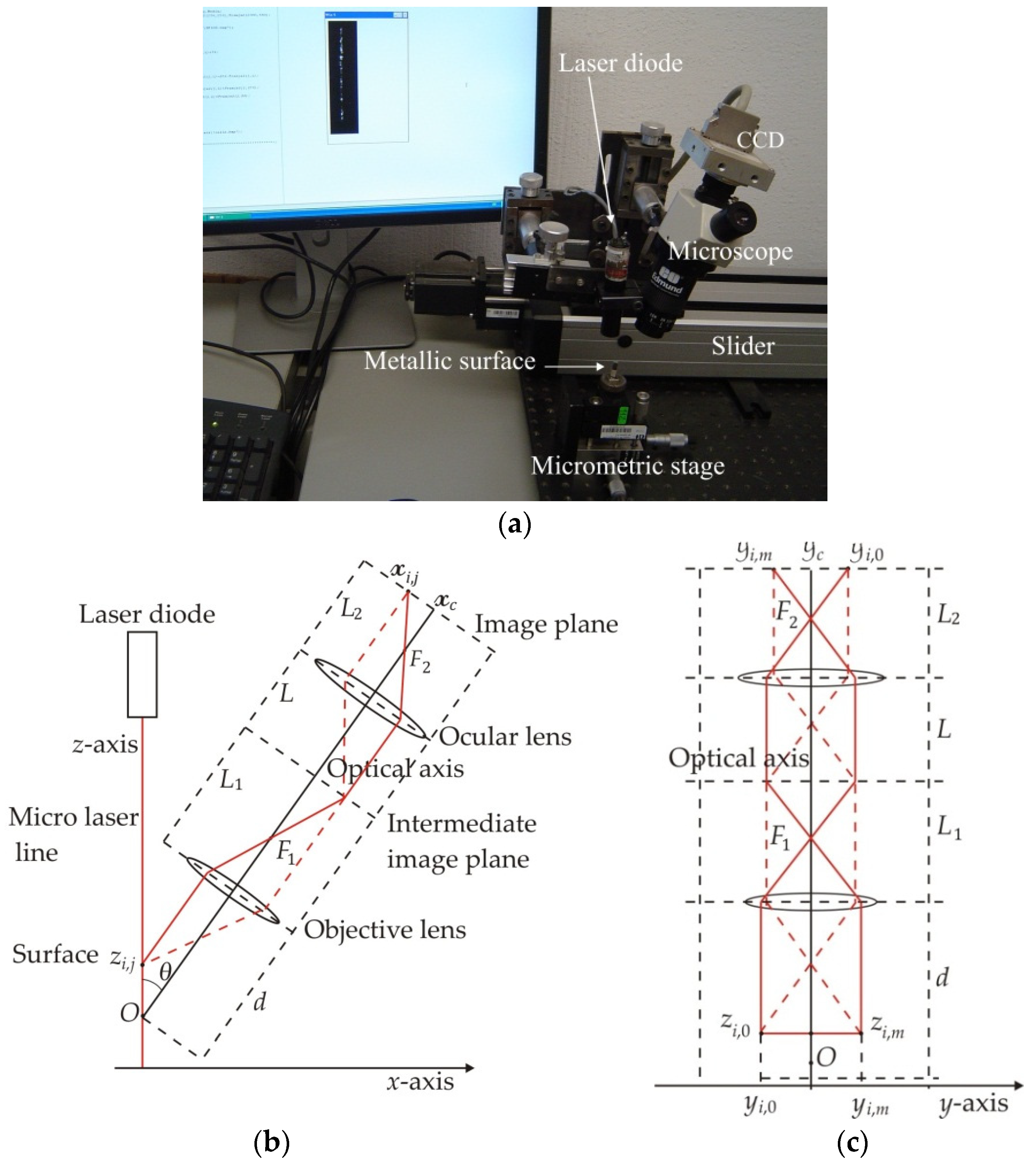
The microscope vision system to perform micro-scale surface contouring is shown in Figure 4a. This arrangement consists of an optical microscope, which includes a laser CCD camera, a diode, and a computer. This microscope system is mounted on a slider device to perform the micro laser scanning. In this arrangement, the surface plane is located on the x-axis and y-axis, and the surface contour is parallel to the z-axis. The lateral view of the microscope arrangement in the x-axis is described by the optical geometry shown in Figure 4b, where a 38 μm laser line is projected perpendicularly on the target surface and the microscope is aligned at an angle. The symbol θ depicts the angle between the optical axis and the laser line. The distance between the surface and the objective lens is defined by d. The objective focal length and the objective focus are represented by L₁ and F₁, respectively. The distance between the ocular lens and the intermediate image plane is represented by L. The ocular focal length and the ocular focus are represented L₂ and F₂, respectively. The lateral view of the microscope arrangement in the y-axis is described by the optical geometry shown in Figure 4c. The laser line coordinates in the image plane are represented by (x_i,j, y_i,j) in the x-axis and y-axis, respectively. The image center is represented by the coordinates (x_c, y_c), and the pixel size is represented by η. The topography coordinates y_i,j and z_i,j are deduced from the geometry shown in Figure 4b,c by means of the expressions

$$z_{i,j}=\frac{\eta (x_c-x_{i,j})F_1{F}_2}{(L_1-F_1)(L_2-F_2)\sin \theta }+O,$$

(15)

$$y_{i,j}=\eta y_c-\frac{\eta (y_c-y_{i,j})F_1{F}_2}{(L_1-F_1)(L_2-F_2)}.$$

(16)

The surface coordinate x_i,j is collected from the position where the laser line is projected in the x-axis. The slider device provides the coordinate in the x-axis. Thus, the topography coordinates are computed through the parameters (x_c, y_c, η, θ, L₁, F₁, L₂, F₂). These vision parameters are determined by a genetic algorithm via Equations (15) and (16) and the topography coordinates. The genetic algorithm computes the vision as follows.

The first step is to compute the initial population from the maximum and minimum of each parameter. In this way, the maximum and minimum of the constants (x_c, y_c, η) are deduced from the image size. However, the maximum and minimum of the variables (θ, L₁, F₁, L₂, F₂) are defined through the microscope geometry. The minimum F₂ is deduced through the ocular lens diameter, and the maximum F₂ is two times the minimum F₂. The minimum L₂ is equal to the minimum F₂, and the maximum L₂ is two times the minimum L₂. Additionally, the minimum F₁ is deduced through the objective lens diameter, and the maximum F₁ is two times the minimum F₁. The minimum L₁ is equal to the minimum F₁, and the maximum L₁ is two times the minimum L₁. The minimum and minimum θ were established as 14° and 40°, respectively. Thus, the solution space is completed. Then, four parents ($\mathcal{P}$_1,k, $\mathcal{P}$_2,k, $\mathcal{P}$_3,k, $\mathcal{P}$_4,k) are computed from the solution space in random form. In this way, the four vision parameters (x_c, y_c, η, θ, L₁, f₁, L₂, f₂) are established as the initial population.

The second step is to perform the crossover to generate the current children. To carry it out, the children (C_1+4*t,k, C_2+4*t,k, C_3+4*t,k, C_4+4*t,k) are computed through the parents ($\mathcal{P}$_1+2*t,k, $\mathcal{P}$_2+2*t,k) for t = 0 and t = 1. Thus, the parents ($\mathcal{P}$_1,k, $\mathcal{P}$_2,k) and t = 0 are replaced in Equation (3) through Equation (6) to compute the children (C_1,k, C_2,k, C_3,k, C_4,k). In the same way, the parents ($\mathcal{P}$_3,k, $\mathcal{P}$_4,k) and q = 1 are substituted in Equation (3) through Equation (6) to compute the children (C_5,k, C_6,k, C_7,k, C_8,k).

The third step is to evaluate the fitness through an objective function, which is deduced from the vision parameters by means of the expressions

$$F{O}_1=\min \left\{\frac{1}{mxn}{{\displaystyle \sum _{i=}^n{\displaystyle \sum _{j=0}^m\left[(z_{i,j}-z_{i,m})-\frac{\eta (x_c-x_{i,j})F_1{F}_2}{(L_1-F_1)(L_2-F_2)\sin \theta }+\frac{\eta (x_c-x_{i,m})F_1{F}_2}{(L_1-F_1)(L_2-F_2)\sin \theta }\right]}}}^2\right\},$$

(17)

$$F{O}_2=\min \left\{\frac{1}{mxn}{{\displaystyle \sum _{i=}^n{\displaystyle \sum _{j=0}^m\left[(y_{i,j}-y_{i,m})+\frac{\eta (y_c-y_{i,j})F_1{F}_2}{(L_1-F_1)(L_2-F_2)}-\frac{\eta (y_c-y_{i,m})F_1{F}_2}{(L_1-F_1)(L_2-F_2)}\right]}}}^2\right\}.$$

(18)

From these objective functions, the fitness is evaluated through the expression FO = (FO₁ + FO₂)/2, where the surface topography (z_i,j − z_i,m) and the surface width (y_i,j − y_i,m) are known.

The fourth step is to select the parents of the next generation from the best current parents and children. In this way, the parents $\mathcal{P}$_1,k+1 and $\mathcal{P}$_3,k+1 are chosen from the parents ($\mathcal{P}$_1,k, $\mathcal{P}$_2,k) and ($\mathcal{P}$_3,k, $\mathcal{P}$_4,k), respectively. Then, the parents $\mathcal{P}$_2,k+1 and $\mathcal{P}$_4,t+1 are chosen from the children (C_1,k, C_2,k, C_3,k, C_4,k) and (C_5,k, C_6,k, C_7,k, C_8,k), respectively.

The fifth step is to perform the mutation to avoid trapping in a local minimum. To carry it out, a new parent is randomly generated from the solution space. Then, the new parent replaces the worst parent, which is selected through the fitness Equations (17) and (18). Thus, if the new parent improves the fitness, the worst parent is replaced by the new parent. Otherwise, the worst parent is not replaced. Additionally, one vision parameter is mutated from a parent, which is selected in random form. To do so, a new vision parameter is randomly generated from the solution space, and it is replaced in the selected parent to compute the fitness by means of Equations (17) and (18). If the new vision parameter improves the fitness, the mutation is carried out; if not, the parameter is not mutated. Thus, the mutation is accomplished to determine the parents of the (k + 1) generation. Then, the children of the (k + 1) generation are generated through the crossover by computing Equation (3) through Equation (6). Additionally, the fitness of these children is computed by means of Equations (17) and (18). From this step, the population of the (k + 1) generation is completed. The steps to determine the (k + 1) generation are repeated until the objective function in Equations (17) and (18) is minimized. Then, the distance from zero to the point O is computed by the expression z_0,j = η(x_0,j − x_c) F₁ F₂/(L₁ − F₁)(L₂ − F₂)sin θ.

The laser line coordinates (x_i,j, y_i,j) are determined through the pixel gray-level. The position x_i,j was determined through the gray-level maximum in the x-axis of the image [38]. In this way, the pixel gray-level is approximated to a Bezier curve in the x-direction by means of the expressions

$$x(u)={\displaystyle \sum _{i=0}^N{\mathcal{C}}_i}{(1-u)}^{N-i}{u}^i{x}_{i,j},\hspace{1em}{\mathcal{C}}_i={\mathcal{C}}_{i-1}(N+1-i)/i,\hspace{1em}{\mathcal{C}}_0=1,\hspace{1em}\hspace{1em}\hspace{1em}0\le u\le 1.$$

(19)

$$I(u)={\displaystyle \sum _{i=0}^N{\mathcal{C}}_i}{(1-u)}^{N-i}{u}^i{I}_{i,j},\hspace{1em}{\mathcal{C}}_i={\mathcal{C}}_{i-1}(N+1-i)/i,\hspace{1em}{\mathcal{C}}_0=1,\hspace{1em}\hspace{1em}\hspace{1em}0\le u\le 1.$$

(20)

In Equation (19), x_i,j represents the laser line coordinates in the x-axis, and N represents the laser line width in pixels. The pixel gray-level is represented by I_i,j in Equation (20), where the sub-index i indicates the pixel number in the x-axis and the sub-index j indicates the pixel number in the y-axis. In this way, x_i,j is substituted in Equation (19) and I_i,j is substituted Equation (20) to compute a concave curve {x(u), I(u)} in the interval 0 ≤ u ≤ 1. Thus, the second derivative I″(u) is positive, and the gray-level maximum is computed through the derivative I′(u) = 0. The value u that provides I′(u) = 0 is computed through the bisection method. By substituting u in Equation (19), x(u) is computed to determine the laser line position x_i,j = x(u) in the x-axis. The laser line position y_i,j is deduced from the row number in the y-axis. Additionally, the line edges y_i,0 and y_i,m are determined by computing the first derivative in the y-axis. In this way, the coordinates (x_i,j, y_i,j) are replaced in Equation (15) and Equation (16) to compute the surface topography (y_i,j, z_i,j) at the micro-scale. To carry it out, the surface is scanned, and a laser line image is captured by the CCD. From this laser line image, the coordinates (x_i,j, y_i,j) are computed by means of Equations (19) and (20). Then, the coordinates (x_i,j, y_i,j) are substituted in Equations (15) and (16) to compute the surface topography (y_i,j, z_i,j). The slider device provides the coordinates x_i,j in the x-axis. Thus, the micro-scale surface coordinates are determined.

3. Results of Micro-Scale Flat and Free-Form Surface Modeling

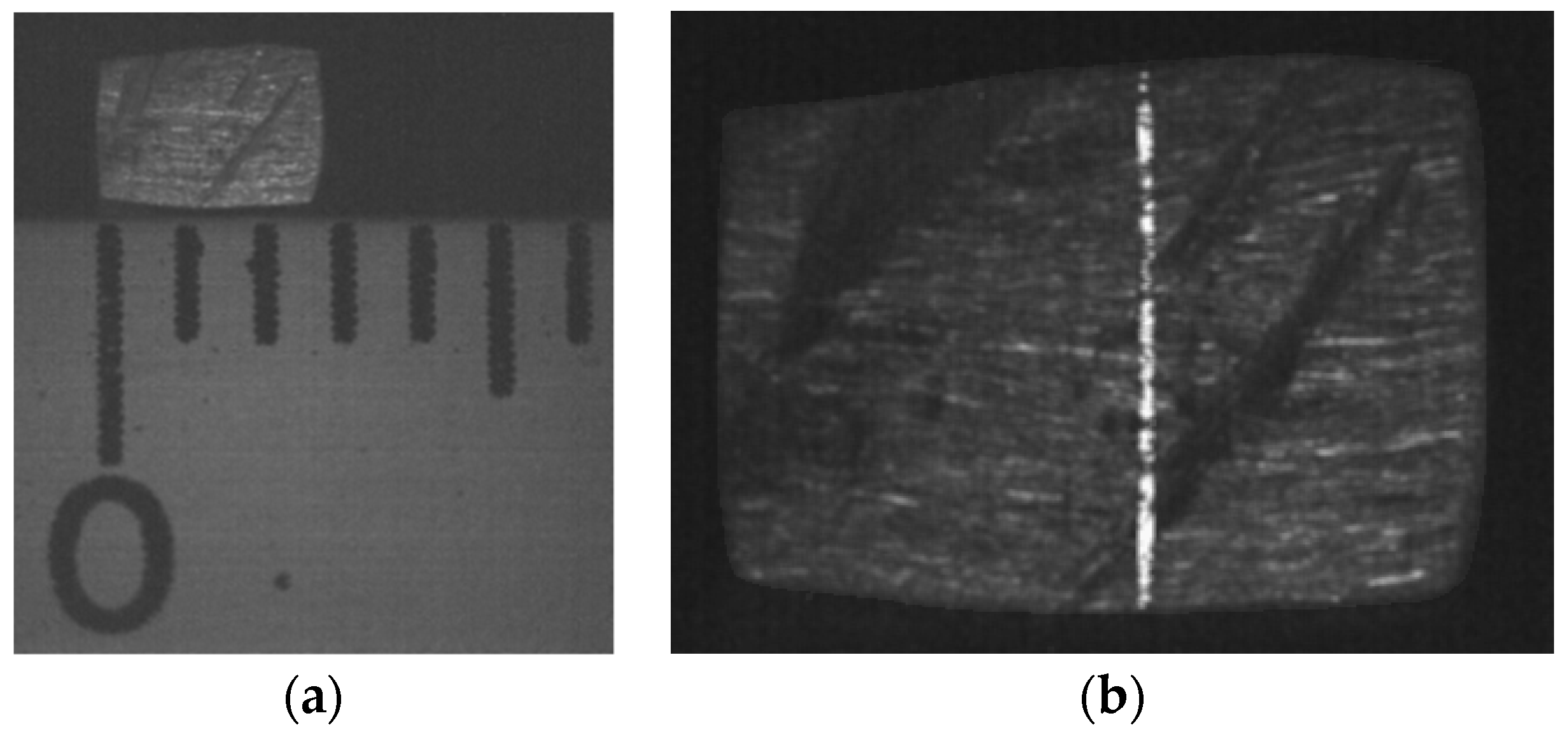
The micro-scale flat and free-form surface modeling was performed through the optical microscope system shown in Figure 4a. The free-form surface modeling at the micro-scale was implemented for the metallic object shown in Figure 5a. In this figure, the scale is indicated in millimeters in the x-axis. Additionally, Figure 5b shows the micro laser line projected on the object surface. In this way, the micro laser line scanned the object surface in the x-axis, and the laser line image was captured by the CCD camera. From the image, the line position coordinates (x_i,j, y_i,j) were computed by means of Equations (19) and (20), respectively. Then, the coordinate x_i,j was substituted in Equation (15) and the coordinate y_i,j was replaced in Equation (16) to compute the surface data (z_i,j, y_i,j). The slider device provided the surface data x_i,j.

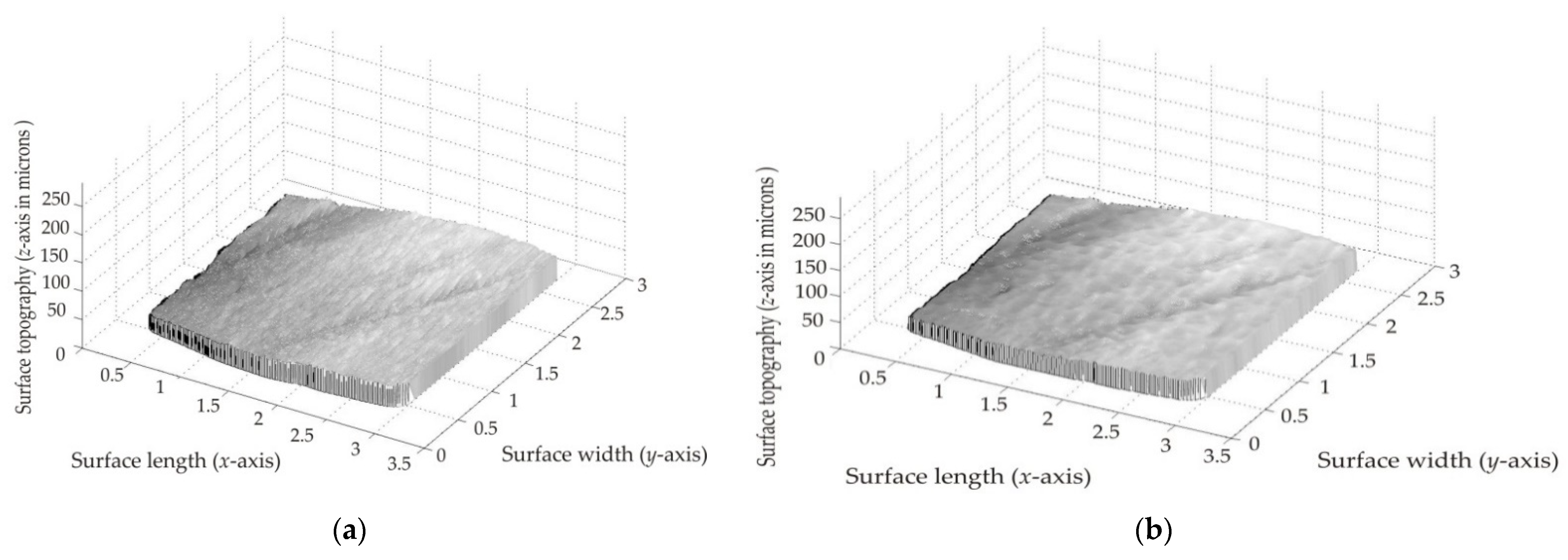
From the scanning, one hundred and sixty-eight images were captured to compute the object topography shown in Figure 6a. In this figure, the x-axis and y-axis are represented in millimeters, but the z-axis is represented in microns. The surface accuracy is computed through the relative error [39], which was calculated via reference data provided by a contact method. In this way, the surface accuracy was determined in terms of percentage by means of the expression

$$Error\%=\frac{100}{n\cdot m}{\displaystyle \sum _{i=0}^n{\displaystyle \sum _{j=0}^m\frac{\left|z_{i,j}-H_{i,j}\right|}{H_{i,j}}}},$$

(21)

In this equation, z_i,j represents the micro-scale surface calculated by means of Equation (15), H_i,j represents the surface reference, and n·m indicates the data number. Thus, Equation (21) was computed by employing the surface data shown in Figure 6a, and the relative error was 0.785%. From the surface shown in Figure 6a, a free-form surface model was constructed through the multi-objective optimization as described in Section 2.1. The steps of this procedure are described as follows.

The first step was to determine the initial population from the solution space of each weight, where the minimum and maximum of the weights were in the interval [0.7, 1.3]. In this way, the genetic algorithm computed four parents in random form from the solution space for each weight of the surface S_p,q(u,v). Then, the second step was to compute the current children through the crossover by replacing t = 0 and t = 1 in Equation (3) through Equation (6). The probability of crossover is deduced by means of the average fitness. Thus, the crossover is performed when the average fitness is enhanced. In this way, the loss of candidates is avoided to achieve the convergence. Then, the third step was to evaluate the fitness by substituting the weights of the parents and children in Equation (1) to compute Equation (7). Then, the fourth step was to select the parents of the next generation from the best current parents and children. Thus, the parents $\mathcal{P}$_1,k+1 and $\mathcal{P}$_3,k+1 were chosen from the pairs ($\mathcal{P}$_1,k, $\mathcal{P}$_2,k) and ($\mathcal{P}$_3,k, $\mathcal{P}$_4,k), respectively. In addition, the parents $\mathcal{P}$_2,t+1 and $\mathcal{P}$_4,t+1 were chosen from the children (C_1,k, C_2,k, C_3,k, C_4,k) and (C_5,k, C_6,k, C_7,k, C_8,k), respectively. Then, the fifth step was to mutate the worst parent, which was selected through the fitness. Thus, if the new parent enhanced the fitness, the worst parent was mutated. Otherwise, the worst parent was not mutated. In addition, one weight was mutated from a parent, which was selected in random form. To do so, a new weight was randomly generated from the solution space, and it was replaced in the selected parent to compute the fitness by means of Equation (7). If the new weight improved the fitness, the mutation was carried out; if not, the weight was not mutated. Then, the second step was carried out by computing Equation (3) through Equation (6) to create the children of the (k + 1) generation. In addition, the fitness of these children was computed by means of Equation (7). From this step, the population of the (k + 1) generation was completed. The steps to determine the (k + 1) generation were repeated until the multi-objective function in Equation (7) was minimized.

The iterations to obtain the optimal weights determine the number of generations. In this case, 174 generations were computed to accomplish the free-form surface model. Thus, the optimal weights were substituted in Equation (1) to obtain the free-form surface model, which generated the object surface shown in Figure 6b. The fitting accuracy of the free-form surface model was determined through the relative error by the expression

$$Error\%=\frac{100}{n\cdot m}{\displaystyle \sum _{i=0}^n{\displaystyle \sum _{j=0}^m\frac{\left|M_{i,j}-z_{i,j}\right|}{z_{i,j}}}},$$

(22)

In this equation, M_i,j represents the micro-scale surface calculated through the free-form surface model Equation (1), z_i,j represents the surface calculated by means of Equation (15), and n·m indicates the number of data. Additionally, the optimal gap of the genetic algorithm was determined by computing the relative error by means of Equation (22). From this step, the free-form surface model produced a relative error of 1.9731% with respect to the metallic surface shown in Figure 6a. The fitness variation indicated that the fitness decreased when the generation number increased.

The efficiency of the multi-objective optimization is described through the parameters in the genetic algorithm as follows. The population size is determined by the number of chromosomes in one generation. In this case, the free-surface model was established through the surface functions S_0,0(u,v), S_1,0(u,v), S_2,0(u,v), …, S_8,7(u,v). Each surface function contained a population of 96 chromosomes. Therefore, one generation included a population of 6912 chromosomes. The crossover probability determines how often the crossover is performed. The probability of crossover is determined via fitness. Thus, the crossover is carried out when the average fitness of the parents is improved. In this way, the multi-objective optimization is performed several times at the same free-form surface model. The result of the probability of crossover was in the interval from 0.27 to 0.53. The mutation probability determines how often the chromosome can be mutated. The mutation probability is determined via fitness. Thus, if the new parent improves the fitness, the worst parent is mutated. In the same way, for the parameter mutation, if the new parameter improves the fitness, the parameter is mutated. Thus, the multi-objective optimization is performed several times on the same free-form surface model. The result of the probability of mutation was in the interval from 0.26 to 0.59. The number of generations indicates the iterations to obtain the optimal control points. In this case, 174 generations were performed to accomplish the free-form surface model. The optimal gap was computed via Equation (22), and the result was a relative error of 1.9731%. Based on these results, the genetic algorithm was examined. For instance, the optimal crossover probability and mutation probability were defined in the interval between 0.3 and 0.6 for surface modeling in recent optimization research [40]. Therefore, the proposed genetic algorithm provided good crossover probability and mutation probability. The population size is related to the convergence and the number of parameters [41]. In this case, the genetic algorithm provided 12 chromosomes for each parameter. These chromosomes produced results near the optimal solution and reduced iterations. Therefore, the algorithm provided a good population size and number of iterations. The optimal gap established good fitting of the surface model to the target surface.

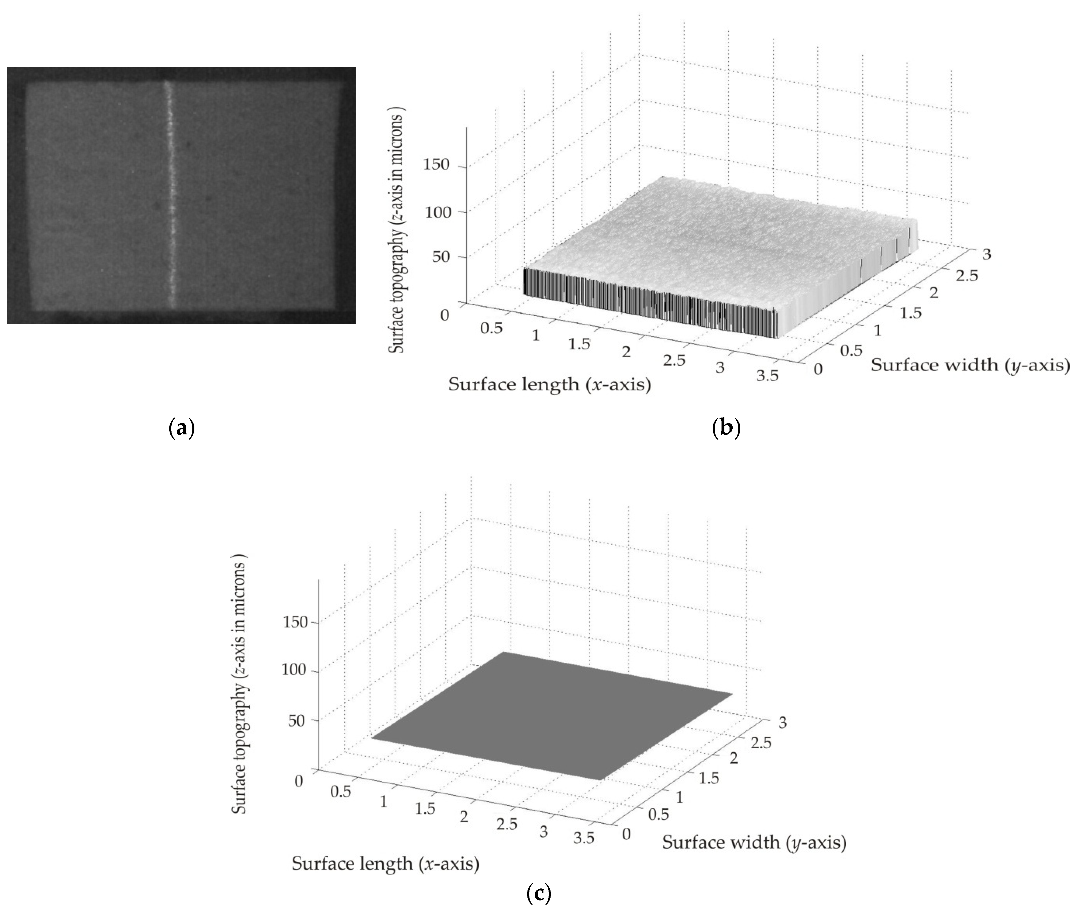
The micro-scale flat surface modeling was carried out for the paper surface shown in Figure 7a. In this way, the paper surface was scanned in the x-axis to retrieve the coordinates (x_i,j, y_i,j) by computing Equations (19) and (20) from the laser line image. Then, the coordinate x_i,j was replaced in Equation (15) and the coordinate y_i,j was replaced in Equation (16) to calculate the surface data (z_i,j, y_i,j). The slider device provided the surface coordinates x_i,j. In this way, one hundred and sixty-four images were captured from the scanning to compute the object topography shown in Figure 7b. In this figure, the x-axis and y-axis are represented in millimeters, but the z-axis is represented in microns. The surface accuracy was computed by means of the relative error Equation (21), where z_i,j represents the surface computed via Equation (15), H_i,j represents the reference data, and n·m indicates the number of data. In this way, Equation (21) was computed by employing the surface data shown in Figure 7a, and the relative error was 0.691%. From this surface, a flat surface model was generated via multi-objective optimization based on a genetic algorithm by means of Equation (8) and the coordinates (x_i,j, y_i,j, z_i,j). The steps of this multi-objective optimization are described as follows.

The first step was to determine the initial population through the coordinates (x_i,j, y_i,j, z_i,j). To carry it out, the initial constants (a, b, c) were computed by means of Equation (11) through Equation (13) as described in Section 2.2. Then, four parents ($\mathcal{P}$_1,1, $\mathcal{P}$_2,1, $\mathcal{P}$_3,1, $\mathcal{P}$_4,1) were computed by employing the sub-indices (i = 0, j = 0, δ = 82, Δ = 80), (i = 82, j = 0, δ = 82, Δ = 80), (i = 0, j = 80, δ = 82, Δ = 80), and (i = 82, j = 80, δ = 82, Δ = 80). In this case, n = 164 and m = 160. Thus, four constants (a, b, c) were obtained, and they were defined as the first parents ($\mathcal{P}$_1,2, $\mathcal{P}$_2,1, $\mathcal{P}$_3,1, $\mathcal{P}$_4,1), where the parent $\mathcal{P}$_1,1 is represented by the constants (a = −0.1061, b = −4.2290, c = 31.1214), the parent $\mathcal{P}$_2,1 is represented by (a = 0.5671, b = −3.672, c = 30.8239), the parent $\mathcal{P}$_3,1 is represented by (a = 0.8934, b = −1.1235, c = 29.1065), and the parent $\mathcal{P}$_4,1 is represented by (a = 0.1432, b = −0.4218, c = 27.8532). Then, the terms (am − 2*as) and (am + 2*as) were computed to determine the maximum and minimum of a. Additionally, the terms (bm − 2*as) and (bm + 2*bs) were computed to determine the maximum and minimum of b, and the terms (cm − 2*cs) and (cm + 2*cs) were computed to determine the maximum and minimum of c. Thus, the initial population was completed. Then, the second step was to determine the current children through the crossover by computing Equation (3) through Equation (6) by employing t = 0 and t = 1. The probability of crossover is deduced via average fitness. Thus, the crossover is performed when the average fitness is enhanced. Next, the third step was to evaluate the fitness by computing Equation (14) using the constants (a, b, c) and the coordinates (x_i,j, y_i,j, z_i,j). Then, the fourth step was to select the parents of the next generation from the best current parents and children, where the parents $\mathcal{P}$_1,k+1 and $\mathcal{P}$_3,k+1 were chosen from the pairs ($\mathcal{P}$_1,k, P_2,k) and ($\mathcal{P}$_3,k, $\mathcal{P}$_4,k), respectively. In addition, the parents $\mathcal{P}$_2,t+1 and $\mathcal{P}$_4,t+1 were chosen from the children (C_1,k, C_2,k, C_3,k, C_4,k) and (C_5,k, C_6,k, C_7,k, C_8,k), respectively. Then, the fifth step was to mutate the worst parent, which was selected through the fitness Equation (14). Thus, if the new parent enhanced the fitness, the worst parent was mutated. Otherwise, the worst parent was not mutated. In addition, one constant was mutated from a parent, which was selected in random form. To do so, a new constant was randomly generated from the solution space, and it was replaced in the selected parent to compute the fitness via Equation (14). If the new constant improved the fitness, the mutation was carried out; if not, the constant was not mutated. Then, the second step was carried out by computing Equation (3) through Equation (6) to create the children of the (k + 1) generation. Additionally, the fitness of these children was computed via Equation (14). From this step, the population of the (k + 1) generation was completed. The steps to compute the (k + 1) generation were repeated until the multi-objective function in Equation (14) was minimized. In this case, the number of generations to obtain the optimal constants (a, b, c) was 157. The optimal constants were a = 0.307, b = −1.983, and c = 28.723, and they were replaced in Equation (8) to determine the flat surface model z_i,j = 0.307x_i,j − 1.983y_i,j + 28.723. This flat surface model produced the flat surface shown in Figure 7c. The fitting accuracy provided by the flat surface model was determined by means of Equation (22) by employing the surface data shown in Figure 7b, where M_i,j represents the surface data provided by the flat surface model Equation (8), z_i,j represents the surface data recovered via Equation (15), and n·m indicates the data number. Additionally, the optimal gap of the genetic algorithm was determined by computing the relative error Equation (22). From this step, the flat surface model produced a relative error of 1.231% with respect to the paper surface shown in Figure 7b.

The running time is defined by the number of generations. In this case, 157 generations were computed to optimize the micro-scale flat surface model. In this way, the micro-scale flat surface modeling was performed through multi-objective optimization. The efficiency of the multi-objective optimization is described through the parameters in the genetic algorithm as follows. The population size is determined through the constants (a, b, c). For each constant, an initial population of twelve chromosomes was generated. Therefore, one generation included a population of 36 chromosomes. The crossover probability determines how often the crossover is performed. When the average fitness of the parents is improved, the crossover is carried out. In this way, the multi-objective optimization is performed several times on the same flat surface model. The result of the probability of crossover was in the interval from 0.21 to 0.55. The mutation probability determines how often the chromosome can be mutated. Thus, if the new parent improves the fitness, the worst parent is mutated. In the same way, for the parameter mutation, if the new parameter improves the fitness, the parameter is mutated. Thus, the multi-objective optimization is performed several times on the same flat surface model. The result of the probability of mutation was in the interval from 0.26 to 0.53. The number of generations indicates the number of the iterations to obtain the optimal constants. In this case, 157 generations were performed to accomplish the flat surface model. The optimal gap was computed via Equation (22), and the result was a relative error of 1.231%. Based on these results, the genetic algorithm was examined. In this case, the genetic provided good crossover probability and mutation probability. It is because the probability was in the interval established in the surface modeling optimization. The population size is related to the convergence and the number of parameters. In this case, the genetic algorithm provided 12 chromosomes for each parameter. These chromosomes produced results near the optimal solution and reduced iterations. Therefore, the algorithm provided a good population size and number of iterations. The optimal gap established good fitting of the surface model to the target surface.

4. Discussion

The viability of surface modeling in industry 4.0 is determined through the fitting accuracy [42]. In this way, the viability of the micro-scale flat and free-form surface modeling is determined through the fitting accuracy [43,44]. Therefore, the contribution of the proposed flat and free-form surface modeling is deduced from the fitting accuracy with respect to the experimental surface data. Additionally, the algorithm efficiency is included in the contribution. In the proposed multi-objective optimization, the fitting accuracy and efficiency provided good results. The fitting accuracy of the flat and free-form surface modeling was deduced through the quality gap, which was calculated by means of Equation (22). Thus, the micro-scale flat and free-form surface modeling performed via multi-objective optimization fit the surface data with an error smaller than 1.99%. On the other hand, the solution quality and algorithm structure determine algorithm efficiency. The algorithm structure optimized the surface model parameters in good manner. It is because the solution space is determined from the surface data, which provide the solution to accomplish the micro-scale flat and free-form surface models. In this way, the algorithm provided an initial population near the optimal parameters. Therefore, a low error was produced by the algorithm from the first generation. Thus, the algorithm reduced iterations to determine the surface model parameters. This led to providing a running time in a moderated number of iterations. In addition, the multi-objective objective function involves several objective functions to perform the optimization via a genetic algorithm. Thus, several solution candidates were obtained to achieve the convergence through the initial population. Based on these statements, the micro-scale flat and free-form surface modeling via multi-objective optimization enhanced the fitting accuracy of the optical microscope systems. Typically, the microscope systems perform the micro-scale flat and free-form surface modeling with a relative error over 4.6% [45,46], where the flat and free-form surface modeling is optimized through the least-squares method [47,48]. Additionally, the contour data accuracy is related to the fitting accuracy of the surface model. Typically, the optical microscope systems determine the topography data through the gray-level to perform the flat and free-form surface modeling [49,50]. However, the surface profile is not depicted by the gray-level profile. Therefore, the surface modeling via contouring based on gray-level does not provide the best fitting accuracy. Instead, micro laser line reflection depicts the micro-scale surface contour with high accuracy. It is because the laser line reflects the surface contour on the microscope image plane. Moreover, the algorithms of artificial intelligence were implemented in industry 4.0 to perform surface modeling [51]. In the same way, flat and free-form surface modeling has been developed through the algorithms of artificial intelligence [52,53]. These algorithms perform the parameter optimization by employing the traditional search structure [54,55], where the solution space is not defined through the data related to the surface model. Instead, the multi-objective optimization determines the solution space by employing contour data related to the surface model. This procedure provides values that produce a low error from the first generation. Thus, the search procedure begins on a path near the optimal parameters. In this way, the iterations to optimize the model parameters are reduced, and the efficiency is enhanced. This statement is corroborated by the low error produced in the initial population. Thus, the multi-objective optimization performs the optimization by employing contour data. Instead, traditional algorithms generate the initial population in random form [56]. It is because the traditional algorithms do not deduce the search space from the surface data. Furthermore, the multi-objective optimization performs a search inside and outside the parents to avoid the elimination of potential solution candidates. This leads to searching in the entire solution space to find the best solution in efficient form. The viability of the multi-objective optimization via a genetic algorithm is elucidated through the fitting accuracy based on the algorithms of artificial intelligence. To elucidate this, intelligent algorithms were employed to perform flat and free-form surface modeling. Thus, the results provided by these algorithms of artificial intelligence are mentioned as follows. The quality gap provided by ant colony and particle swarm optimization was over 4.23%. These methods performed more than 235 generations to accomplish the flat and free-form surface models. The suitable structure is discussed based on the structure of the particle swarm, which has been implemented to perform surface modeling in industry 4.0. For instance, the particle swarm determines the population through the learning factors, which are described as follows. In this way, the particle swarm performs the population evolution based on two learning factors (α, β), two random numbers (R₁, R₂), and an inertia weight w [57]. Therefore, the particle swarm should compute five variables to determine the population of each generation. Instead, the proposed algorithm computes the variable β through the spread factor α to create the population of each generation. Thus, the suitable structure of the multi-objective optimization via genetic algorithms provides a better efficiency than the particle swarm. In addition, the proposed genetic algorithm computes minus variables than simulated annealing and ant colony to optimize flat and free-form surface models. Based on these statements, the multi-objective optimization based on the genetic algorithm elucidates a suitable structure to construct flat and free-form surface models. This criterion was elucidated through the surface models optimized by particle swarm optimization and genetic algorithms [58]. Thus, the capability of the micro-scale flat and free-form surface modeling via multi-objective optimization is corroborated. Finally, the efficiency of the multi-objective optimization is elucidated through the parameters in the genetic algorithm. The population size is determined by the number of chromosomes of one generation. For instance, the free-form surface model included a population of 6912 chromosomes, and the flat surface model included 36 chromosomes in one generation. However, in both cases, the initial population provided data near the optimal solution. Therefore, a good convergence was achieved. This means that the algorithm provided a good population size in each generation. The crossover probability determines how often the crossover is performed. The mutation probability determines how often the chromosome can be mutated. Based on the results, the genetic algorithm provided a probability of crossover and mutation in and around the interval between 0.25 and 0.6, which was established by recent optimization research. Therefore, the proposed genetic algorithm provided a good crossover probability and mutation probability. The structure of the genetic algorithm reduced iterations. Based on the results described, the genetic algorithm provided a good number of iterations to optimize the model parameters. The optimal gap established good fitting of the surface model to the target surface. It is corroborated with respect to the particle swarm, which performs surface modeling. In addition, the multi-objective optimization via genetic algorithms provides a contribution with respect to our spherical and cylindrical surface modeling, which is referenced in Figure 4. It is because our spherical and cylindrical surface models are represented by just one equation. In this way, the free-form surface model does not fit accurately to the surface when the model is constructed by employing one equation. Therefore, it is necessary to construct the free-form surface model through multi-functions, which fits accurately to surface data. Additionally, the simple optical arrangement provides a low cost to increase the capability of the proposed micro-scale flat and free-form surface modeling. Thus, the multi-objective optimization based on a genetic algorithm and micro laser line projection makes a contribution in the field of flat and free-form surface modeling, which is performed by the optical microscope systems.

The micro-scale flat and free-form surface modeling was implemented in a computer at a velocity of 2.2 GHz. Additionally, the computer performed the control of the CCD camera, which captured 58 images per second. In addition, the slider device was moved by the computer through control software. In this way, the surface contour was recovered in 0.0052 s from each micro laser line image. Additionally, the time to perform the surface modeling was defined by including the surface recovering via laser line scanning. Thus, the free-form surface model of the metallic surface was performed in 67.57 s, and the flat surface model of the paper surface was carried out in 48.36 s.

5. Conclusions

A technique to perform flat and free-form surface modeling through the multi-objective optimization and micro laser line scanning was presented. The multi-objective optimization enhanced the fitting accuracy of the flat and free-form surface models, which was performed by the optical microscope system. This capability was elucidated through the algorithm efficiency and fitting accuracy to optimize flat and free-form surface models. The enhancement of the fitting accuracy was achieved through the algorithm structure, which accurately approximated the model to the micro-scale flat and free-form surfaces. Additionally, the improvement in fitting accuracy was given by the micro laser line scanning. It is because the laser line accurately reflects the surface topography on the microscope image plane. In this way, the micro-scale flat and free-form surface models were constructed through the real surface contour. The multi-objective efficiency was achieved through the solution space, which provided initial solutions with low error to achieve the optimal surface model. Thus, the iterations were reduced to accurately fit the flat and free-form surface models. Thus, the multi-objective optimization via a genetic algorithm proves valuable in industry 4.0 to perform flat and free-form surface modeling in the field of optical microscope systems. In addition, the optical microscope arrangement included simple components such as: an optical microscope, a diode laser, and a CCD camera. This led to reduced cost of the optical arrangement, and it corroborates the capability of the micro-scale flat and free-form surface modeling. Thus, the multi-objective optimization via genetic algorithms and micro laser line scanning was implemented to perform micro-scale flat and free-form surface modeling, with good results in the micro-scale interval.

References

1. Ghosh, A.K.; Ullah, A.S.; Kubo, A.; Akamatsu, T.; D’Addona, D.M. Machining phenomenon twin construction for Industry 4.0: A Case of Surface Roughness. J. Manuf. Mater. Process. 2020, 4, 11. [Google Scholar] [CrossRef]
2. Villalonga, A.; Beruvides, G.; Castaño, F.; Haber, R.E. Cloud-Based Industrial Cyber–physical system for data-driven reasoning: A review and use case on an Industry 4.0 Pilot Line. IEEE Trans. Ind. Inform. 2020, 16, 5975–5984. [Google Scholar] [CrossRef]
3. Gan, B.; Zhang, C.; Chen, Y.; Chen, Y.C. Research on role modeling and behavior control of virtual reality animation interactive system in Internet of Things. J. Real-Time Image Process. 2021, 18, 1069–1083. [Google Scholar] [CrossRef]
4. Nasr, M.M.; Anwar, S.; Al-Samhan, A.M.; Ghaleb, M.; Dabwan, A. Milling of graphene reinforced Ti6Al4V nanocomposites: An artificial intelligence based industry 4.0 approach. Materials 2020, 13, 5707. [Google Scholar] [CrossRef] [PubMed]
5. Majstorovic, V.; Stojadinovic, S.; Zivkovic, S.; Djurdjanovic, D.; Jakovljevic, Z.; Gligorijevic, N. Cyber-physical manufacturing metrology model (CPM3) for sculptured surfaces–turbine blade application. Procedia CIRP 2017, 63, 658–663. [Google Scholar] [CrossRef]
6. Elhoone, H.; Zhang, T.; Anwar, M.; Desai, S. Cyber-based design for additive manufacturing using artificial neural networks for Industry 4.0. Int. J. Prod. Res. 2020, 58, 2841–2861. [Google Scholar] [CrossRef]
7. Czimmermann, T.; Chiurazzi, M.; Milazzo, M.; Roccella, S.; Barbieri, M.; Dario, P. An autonomous robotic platform for manipulation and inspection of metallic Surfaces in Industry 4.0. IEEE Trans. Autom. Sci. Eng. 2022, 19, 1691–1706. [Google Scholar] [CrossRef]
8. Mishra, D.; Roy, R.B.; Dutta, S.; Pal, S.K.; Chakravarty, D. A review on sensor based monitoring and control of friction stir welding process and a roadmap to Industry 4.0. J. Manuf. Process. 2018, 36, 373–397. [Google Scholar] [CrossRef]
9. Yan, J.; Meng, Y.; Lu, L.; Li, L. Industrial big data in an Industry 4.0 environment: Challenges, schemes, and applications for predictive maintenance. IEEE Access 2017, 5, 23484–23491. [Google Scholar] [CrossRef]
10. Nadolny, K.; Kapłonek, W. Analysis of flatness deviations for austenitic stainless steel work pieces after efficient surface machining. Meas. Sci. Rev. 2014, 14, 204–212. [Google Scholar] [CrossRef] [Green Version]
11. Fei, W.; Narsilio, G.A.; Disfani, M.M. Impact of three-dimensional sphericity and roundness on heat transfer in granular materials. Powder Technol. 2019, 355, 770–781. [Google Scholar] [CrossRef]
12. Zheng, Y. A simple unified branch-and-bound algorithm for minimum zone circularity and sphericity errors. Meas. Sci. Technol. 2020, 31, 045005. [Google Scholar] [CrossRef]
13. Lei, L.; Xie, Z.; Zhu, H.; Guan, Y.; Kong, M.; Zhang, B.; Fu, Y. Improved particle swarm optimization algorithm based on a three–dimensional convex hull for fitting a screw thread central axis. IEEE Access 2021, 9, 4902–4910. [Google Scholar] [CrossRef]
14. Brad, E.; Brad, S. Algorithm for designing reconfigurable equipment to enable Industry 4.0 and circular economy-driven manufacturing systems. Appl. Sci. 2021, 11, 4446. [Google Scholar] [CrossRef]
15. Ding, Y.; Zhang, W.; Yu, L.; Lu, K. The accuracy and efficiency of GA and PSO optimization schemes on estimating reaction kinetic parameters of biomass pyrolysis. Energy 2019, 176, 582–588. [Google Scholar] [CrossRef]
16. Lodewijks, G.; Cao, Y.; Zhao, N.; Zhang, H. Reducing CO2 emissions of an airport baggage handling transport system using a particle swarm optimization algorithm. IEEE Access 2021, 9, 121894–121905. [Google Scholar] [CrossRef]
17. Saini, D.; Kumar, S.; Singh, M.K.; Ali, M. Two view NURBS reconstruction based on GACO model. Complex Intell. Syst. 2021, 7, 2329–2346. [Google Scholar] [CrossRef]
18. Tran, N.-H.; Park, H.S.; Nguyen, Q.V.; Hoang, T.D. Development of a smart cyber-physical manufacturing system in the Industry 4.0 Context. Appl. Sci. 2019, 9, 3325. [Google Scholar] [CrossRef]
19. Soori, M.; Asmael, M. A review of the recent development in machining parameter optimization. Jordan J. Mech. Ind. Eng. 2022, 16, 205–223. [Google Scholar]
20. Ye, X.; Luo, L.; Hou, L.; Duan, Y.; Wu, Y. Laser ablation manipulator coverage path planning method based on an improved ant colony algorithm. Appl. Sci. 2020, 10, 8641. [Google Scholar] [CrossRef]
21. Pathak, V.K.; Nayak, C.; Singh, R.; Dikshit, M.K.; Sai, T. Optimizing parameters in surface reconstruction of transtibial prosthetic socket using central composite design coupled with fuzzy logic-based model. Neural Comput. Appl. 2020, 32, 15597–15613. [Google Scholar] [CrossRef]
22. Kannan, K.; Arunachalam, N.; Chawla, A.; Natarajan, S. Multi-sensor data analytics for grinding wheel redress life estimation- an approach towards Industry 4.0. Procedia Manuf. 2018, 26, 1230–1241. [Google Scholar] [CrossRef]
23. Florková, Z.; Jambor, M. Quantification of aggregate surface texture based on three dimensional microscope measurement. Procedia Eng. 2017, 192, 195–200. [Google Scholar] [CrossRef]
24. Bustillo, A.; Pimenov Yu, D.; Mia, M.; Kapłonek, W. Machine-learning for automatic prediction of flatness deviation considering the wear of the face mill teeth. J. Intell. Manuf. 2021, 32, 895–912. [Google Scholar] [CrossRef]
25. Melentiev, R.; Fang, F. Tailoring of surface topography for tribological purposes by controlled solid particle impacts. Wear 2020, 444–445, 203164. [Google Scholar] [CrossRef]
26. Haitjema, H. Straightness, flatness and cylindricity characterization using discrete Legendre polynomials. CIRP Ann.-Manuf. Technol. 2020, 69, 457–460. [Google Scholar] [CrossRef]
27. Vidal, M.; Ostra, M.; Imaz, N. García-Lecina, E.; Ubide, C. Feature descriptors from scanned images of chromium electrodeposits as predictor parameters of surface roughness and crystallographic texture. Chemom. Intell. Lab. Syst. 2015, 149, 90–98. [Google Scholar] [CrossRef]
28. Shaukat, N.; Ahmad, A.; Mohsin, B.; Khan, R.; Ud-Din Khan, S.; Ud-Din Khan, S. Multi objective core reloading pattern optimization of PARR-1 using modified genetic algorithm coupled with Monte Carlo methods. Sci. Technol. Nucl. Install. 2021, 2021, 1802492. [Google Scholar] [CrossRef]
29. Melin, P.; Sánchez, D. Multi-objective optimization for modular granular neural networks applied to pattern recognition. Inf. Sci. 2018, 460–461, 594–610. [Google Scholar] [CrossRef]
30. Akleman, E.; Srinivasan, V.; Chen, J. Interactive modeling of smooth manifold meshes with arbitrary topology: G1 stitched bi-cubic Bézier patches. Comput. Graph. 2017, 66, 64–73. [Google Scholar] [CrossRef]
31. Long, Q.; Wu, C.; Wang, X.; Huang, T.; Wang, X. A genetic algorithm for unconstrained multi-objective optimization. Swarm Evol. Comput. 2015, 22, 1–14. [Google Scholar] [CrossRef]
32. Jia, L.; Cheng, D.; Chiu, M.S. Pareto-optimal solutions based multi-objective particle swarm optimization control for batch processes. Neural Comput. Appl. 2012, 21, 1107–1116. [Google Scholar] [CrossRef]
33. Hazra, J.; Sinha, A.K. Congestion Management Using Multiobjective Particle Swarm Optimization. IEEE Trans. Power Syst. 2007, 22, 1726–1734. [Google Scholar] [CrossRef]
34. Tan, K.C.; Chiam, S.C.; Mamun, A.A.; Goh, C.K. Balancing exploration and exploitation with adaptive variation for evolutionary multi–objective optimization. Eur. J. Oper. Res. 2009, 197, 701–713. [Google Scholar] [CrossRef]
35. Li, C.Y.; Zhu, C.G. G1 continuity of four pieces of developable surfaces with Bézier boundaries. J. Comput. Appl. Math. 2018, 329, 164–172. [Google Scholar] [CrossRef]
36. Tao, P.; Sun, Z.; Sun, Z. An improved intrusion detection algorithm based on GA and SVM. IEEE Access 2018, 6, 13624–13631. [Google Scholar] [CrossRef]
37. Muñoz-Rodríguez, J.A. Micro-scale spherical and cylindrical surface modeling via metaheuristic algorithms and micro laser line projection. Algorithms 2022, 15, 145. [Google Scholar] [CrossRef]
38. Muñoz-Rodríguez, J.A.; Rodríguez-Vera, R. Evaluation of the light line displacement location for object shape detection. J. Mod. Opt. 2003, 50, 137–154. [Google Scholar] [CrossRef]
39. Yu, H.; Huang, Q.; Zhao, J. Fabrication of an optical fiber micro-sphere with a diameter of several tens of micrometers. Materials 2014, 7, 4878–4895. [Google Scholar] [CrossRef]
40. Lin, T.W.; Wang, C.H. A hybrid genetic algorithm to minimize the periodic preventive maintenance cost in a series-parallel system. J. Intell. Manuf. 2012, 23, 1225–1236. [Google Scholar] [CrossRef]
41. Gibbs, M.S.; Maier, H.R.; Dandy, G.C. Relationship between problem characteristics and the optimal number of genetic algorithm generations. Eng. Optim. 2011, 43, 349–376. [Google Scholar] [CrossRef]
42. Cheng, X. Algorithm of CAD surface generation for complex pipe model in Industry 4.0 background. Comput. Intell. Neurosci. 2022, 2022, 7062052. [Google Scholar] [CrossRef] [PubMed]
43. Kovács, Z.F.; Viharos, Z.J.; Kodácsy, J. Surface flatness and roughness evolution after magnetic assisted ball burnishing of magnetizable and non-magnetizable materials. Measurement 2020, 158, 107750. [Google Scholar] [CrossRef]
44. Rena, M.J.; Suna, L.J.; Liub, M.Y.; Cheungb, C.F.; Yina, Y.H.; Cao, Y.L. A weighted least square based data fusion method for precision measurement of freeform surfaces. Precis. Eng. 2017, 48, 144–151. [Google Scholar] [CrossRef]
45. Miko, B. Assessment of flatness error by regression analysis. Measurement 2021, 171, 108720. [Google Scholar] [CrossRef]
46. Mikó, B.; Varga, B.; Zębala, W. The effect of the feed direction on the micro- and macro accuracy of 3D ball-end milling of chromium-molybdenum Alloy Steel. Materials 2019, 12, 4038. [Google Scholar] [CrossRef]
47. Ye, L.; Qian, J.; Haitjema, H.; Reynaerts, D. On-machine chromatic confocal measurement for micro-EDM drilling and milling. Precis. Eng. 2022, 76, 110–123. [Google Scholar] [CrossRef]
48. Zhu, D.; Feng, X.; Xu, X.; Yang, Z.; Li, W.; Yan, S.; Ding, H. Robotic grinding of complex components: A step towards efficient and intelligent machining–challenges, solutions, and applications. Robot. Comput.-Integr. Manuf. 2020, 65, 101908. [Google Scholar] [CrossRef]
49. Fang, H.; Zhu, H.; Yang, J.; Huang, X.; Hu, X. Three-dimensional angularity characterization of coarse aggregates based on experimental comparison of selected methods. Part. Sci. Technol. 2021, 1, 1–9. [Google Scholar] [CrossRef]
50. Chen, L.C. Automatic 3D surface reconstruction and sphericity measurement of micro spherical balls of miniaturized coordinate measuring probes. Meas. Sci. Technol. 2007, 18, 1748–1755. [Google Scholar] [CrossRef]
51. Stojadinovic, S.M.; Majstorovic, V.D.; Gąska, A.; Sładek, J.; Durakbasa, N.M. Development of a coordinate measuring machine—based inspection Planning system for industry 4.0. Appl. Sci. 2021, 11, 8411. [Google Scholar] [CrossRef]
52. Shu, H.; Zou, C.; Chen, J.; Wang, S. Research on micro/nano surface flatness evaluation method based on improved particle swarm optimization algorithm. Front. Bioeng. Biotechnol. 2021, 9, 775455. [Google Scholar] [CrossRef]
53. Yang, Y.; Dong, Z.; Meng, Y.; Shao, C. Data-driven intelligent 3D surface measurement in smart manufacturing: Review and outlook. Machine 2021, 9, 13. [Google Scholar] [CrossRef]
54. Liang, Z.; Liu, X.; Ye, B.; Wang, Y. Performance investigation of fitting algorithms in surface micro-topography grinding processes based on multi-dimensional fuzzy relation set. Int. J. Adv. Manuf. Technol. 2013, 67, 2779–2798. [Google Scholar] [CrossRef]
55. Tian, X.; Kong, L.; Kong, D.; Yuan, L.; Kong, D. An improved method for NURBS surface based on particle swarm optimization BP neural network. IEEE Access 2020, 8, 184656–184663. [Google Scholar] [CrossRef]
56. Wu, Z.; Wang, X.; Fu, Y.; Shen, J.; Jiang, Q.; Zhu, Y.; Zhou, M. Fitting scattered data points with ball B-Spline curves using particle swarm optimization. Comput. Graph. 2018, 72, 1–11. [Google Scholar] [CrossRef]
57. Tsiptsis, I.N.; Liimatainen, L.; Kotnik, T.; Niiranen, J. Structural optimization employing isogeometric tools in Particle Swarm Optimizer. J. Build. Eng. 2019, 24, 100761. [Google Scholar] [CrossRef]
58. Wang, S.; Xia, Y.; Wang, R.; You, L.; Zhang, J. Optimal NURBS conversion of PDE surface-represented high-speed train heads. Optim. Eng. 2019, 20, 907–928. [Google Scholar] [CrossRef] [Green Version]
Figure 1. Free-form surface data to perform surface modeling.
Energies 15 06571 g001
Figure 2. (a) Contour data to construct free-form surface model. (b) Flowchart to perform multi-objective optimization through a genetic algorithm. (c) Surface generated by the free-form surface model Equation (1).
Energies 15 06571 g002
Figure 3. Surface coordinates to perform flat surface modeling.
Energies 15 06571 g003
Figure 4. (a) Microscope vision system to compute micro-scale flat and free-form topography [37]. (b) Lateral geometry of the microscope system in x-axis. (c) Geometry of the microscope system in y-axis.
Energies 15 06571 g004
Figure 5. (a) Metallic object surface with scale in mm in x-axis. (b) Micro laser line projected on the object surface.
Energies 15 06571 g005
Figure 6. (a) Micro-scale topography recovered via micro laser line scanning. (b) Object surface computed by the free-form surface model generated via Equation (1).
Energies 15 06571 g006
Figure 7. (a) Micro laser line projected on flat surface to perform micro-scale flat surface modeling. (b) Micro-scale surface retrieved via micro laser line scanning. (c) Surface computed by the flat surface model generated via Equation (8).
Energies 15 06571 g007