Abstract
This paper presents an experimental platform for regulating the DC motor angular speed powered by photovoltaic cells. The experimental platform comprises an Eco Green Energy EGE-260P-60 solar panel, DC/DC SEPIC converter, DC bus, DC/DC buck converter, DC motor and Nexys 4 board with an Artix-7 100T FPGA. The DC/DC SEPIC converter is used for harvesting the maximum amount of energy from the PV cells using the perturb and observe algorithm to track the maximum power point. The DC/DC buck converter is used as the motor drive using the active disturbance rejection control to regulate the angular speed of the DC motor. In addition, the FPGA architecture design is presented using a hierarchical top-down methodology with the VHDL hardware description language and Xilinx System Generator tool. The software takes advantage of the FPGA’s concurrency to simultaneously evaluate the different processes, which is the main reason for choosing this digital device. Several tests were performed on the platform such as irradiance changes, DC bus variations, DC motor connection and load torque variations applied in the motor shaft. The results indicate that the maximum power is obtained from the photovoltaic cells, establishing the minimum operating conditions. In addition, the control approach estimates and cancels the effects of disturbances caused by variations in the environmental conditions, photovoltaic system, DC bus, and load changes in order to regulate DC motor speed.
1. Introduction
In recent years, the environmental problems caused by conventional energy sources have become major concerns due to the emission of greenhouse gases and the depletion of energy sources [1,2]. In addition, electric motor drive systems are the largest source of power consumption, representing more than 40% of the global consumption [3,4]. Therefore, innovation in sustainable energy supply is essential in order to provide reliable and clean energy sources, in which a motor plays a prominent role [5]. One of the most appealing renewable energy sources is photovoltaic (PV) solar energy because it is an inexhaustible source of energy present on the entire surface of the earth, which is suitable for isolated locations and has low installation and maintenance costs. As a result, solar PV energy is a viable option for replacing conventional energies, especially in areas with a high solar radiation [6,7].
However, PV cells are non-linear energy sources that depend on environmental conditions. PV cells have a maximum power point (MPP) at which the transformation of solar energy into electrical energy is maximized [8,9]. The MPP involves maximum energy harvesting; therefore, it is essential to find this point through Maximum Power Point Tracking (MPPT) techniques using a suitable converter topology. A large number of MPPT techniques have been developed, including advanced techniques, such as fuzzy logic control [10,11]; ant colony optimization-based [12,13]; differential evolution-based [14]; moth-flame optimization-based [15,16]; artificial neural networks [17,18]; and adaptation of conventional techniques [19,20]. The reviews of [21,22,23] draw comparisons in terms of the speed and accuracy of MPP tracking, the sensors required, the software and resources used, the complexity of implementation, and the overall cost. As a result, the perturb and observe (P&O) algorithm is the most widely used technique because of it is simple to operate, uses few resources, and is easy to implement.
Regarding the DC/DC converter topology, refs. [24,25,26] present reviews on the different isolated and non-isolated MPPT topologies. In this context, the buck-boost, Cuk and SEPIC converters are the most suitable topologies for this purpose. As a result, the SEPIC converter is the most practical to use because its output voltage has the same polarity as the input voltage, while the other two topologies invert it.
The state-of-the-art DC motor drives powered by DC power supplies in recent years are as follows: Yang and Li [27] proposed a robust predictive speed regulation of a permanent magnet DC motor driven by the DC/DC buck converter, where the DS1103 dSPACE board is used to implement the proposed closed-loop feedback control scheme. Hoyos et al. [28] presented the zero-average dynamics and fixed-point induction control approaches to regulate the speed of a DC motor using the DC/DC buck converter as the motor drive, where the DS1104 dSPACE board was used. Nizami et al. [29] proposed a Hermite neural network (HNN) scheme for the angular speed tracking of a permanent magnet DC motor driven by a DC/DC buck converter. The scheme consists of an HNN combined with on-board adaptive learning to counteract the unknown non-linear time-varying load torque, where the TM320F240 DSP and the dSPACE DS1103 boards are used. Alajmi et al. [30] proposed a small signal control to regulate the angular speed of a permanent magnet DC motor using the DC/DC boost converter for electric vehicle applications, where the control approach was implemented using the DS1103 dSPACE board. Hernandez-Marquez et al. [31] proposed a robust hierarchical tracking controller for a system that comprises a bidirectional DC/DC buck–boost converter, an inverter and a DC motor. This controller considers a high-level control for the inverter-DC motor subsystem and a low-level control for the DC/DC buck–boost converter subsystem. Both controllers are experimentally implemented on a prototype using the DS1104 dSPACE board. Guerrero et al. [32] proposed a robust speed controller of a DC motor driven by the parallel–DC/DC buck converter from the perspective of generalized proportional integral (GPI) observers and the active disturbance rejection control (ADRC). A rapid prototyping tool is used for synthetizing the proposed controller into a field-programmable gate array (FPGA) using the Matlab/Simulink and Xilinx System Generator (XSG) tools.
The related studies that focus on PV energy are the following: Kottas et al. [33] proposed the speed regulation of a DC motor using a system that comprises the PV cells, three DC/DC buck–boost converters and an auxiliary storage energy system (batteries). The fuzzy cognitive network and a fuzzy controller were used in order to regulate the speed of the DC motor by adjusting its load–speed characteristics, whereby batteries were used to supply or absorb the remaining energy. Therefore, the system has higher costs because of the multiple additional stages involved if its main function is to regulate the speed. Viji et al. [34] proposed a DC motor speed regulation technique using a system that comprises PV cells, a DC/DC boost converter and a chopper converter as the motor drive. This system uses the P&O algorithm to track the MPP and the discrete sliding mode theory to control the speed of the DC motor. This was a simulation study in which irradiance does not significantly vary, meaning that changes in environmental conditions were not reflected in the operating conditions. Silva-Ortigoza et al. [35] proposed the speed regulation of the DC motor powered by a PV emulator using a DC/DC buck converter. This system uses a robust flatness-based approach to regulate the DC motor speed, although the trade-off is that it does not provide MPP tracking. However, the negative effects of ignoring the MPPT are not reflected because a controlled PV emulator is used to replace the PV cells, which can easily adapt to suitable conditions. The experiment was carried out using the TDK-Lambda G100-17 programmable DC power supply and the DS1104 dSPACE board.
Other studies related to a photovoltaic energy power supply with MPPT approaches are presented in [36,37,38,39,40,41,42]. In contrast with previous research, modern studies focus on pumping applications or speed regulation using AC motor drives. The systems have several aspects in common despite the use of different converter topologies, motors and control theories:
- Two stages of power electronic converters are required: one is used to track the MPP and the other is the motor drive.
- In cases where only a single converter is used, a control objective is then lost, either through obtaining the MPP of the PV cells or regulating the motor speed. Most of the systems prefer to track the MPP over speed regulation, as these systems are designed for pumping water, where it is important to take advantage of the maximum available energy. The P&O and INC algorithms are the most commonly used MPPT techniques.
- A DC bus is always used, either between the PV cells and the single converter, or between the power electronic converters if more than one is used in the system.
- Motor drivers are directly powered by the DC bus, as this is a better way of harnessing DC power than in DC/AC/DC transformations.
Discussion of Related Studies, Motivation and Contributions
The studies in [27,28,29,30,31] present different control schemes for the regulation and tracking tasks of DC motor drives when regulated DC power supplies are used. In these studies, the dSPACE board is most commonly used to implement these controllers. However, the dSPACE board is more expensive than other digital solutions such as microprocessors, application-specific integrated circuits or FPGAs. Therefore, the dSPACE board increases the cost and system size and has limited functionality, for example, a low sampling frequency and large execution time. As a result, an FPGA is an excellent option to implement the control approach because the software takes advantage of the FPGA’s ability to simultaneously evaluate the P&O algorithm and ADRC approach, which is the main reason for choosing this digital device [43,44].
The studies in [33,34,35,36,37,38,39,40,41,42] show that it is essential to track the MPP in order to harvest the maximum energy of the PV cells, where the P&O algorithm is the most widely used. The main difference between these studies lies in the manner in which the motor speed is controlled. In this sense, it is necessary to consider that solar energy is a variable power supply, and a suitable control approach is needed against changes in voltage and current caused by power supply dynamics.
One of the control approaches that has been tested for systems with variable and unknown dynamics is the ADRC approach. The idea behind this approach is to include all nonlinearities along with external and internal disturbances into a single term, which is estimated by a GPI observer. Then, the negative effects of the estimated term are canceled out in a linear control law. The ADRC approach has been successfully applied in converters [45,46]; motor control [32,47]; liquid level control [48]; robotics [49,50]; hydraulic systems [51]; and PV systems [52]; among others. In these studies, the ADRC approach has a satisfactory performance and shows that it is suitable for the proposed system.
Based on the aforementioned studies, this paper presents an experimental platform using two power electronic converters in order to harvest the maximum amount of energy from the PV cells and to control the DC motor. The control approach uses the perturb and observe algorithm to track the MPP of the PV cells and the ADRC to regulate the angular speed of the DC motor. In contrast to [27,28,29,30,31,32,35], this paper uses PV cells instead of a traditional DC power supply or a PV emulator. In addition, the control approach is focused on speed regulation by taking advantage of MPP tracking, as opposed to pumping applications in [36,37,38,39,40,41,42], where the angular speed is not regulated. Therefore, the scientific contribution of this paper focuses on two aspects: the first aspect is applying the ADRC approach to regulate the motor speed, while it is powered by a PV system with maximum energy harvesting, which has not yet been reported in the literature. The control approach estimates and cancels the effects of variations in the environmental conditions, photovoltaic system, DC bus, and load changes in order to regulate the DC motor speed. The second contribution shows the FPGA architecture design in detail to implement the control approach using a hierarchical top-down methodology, where the procedure design is supported by the openly available supplementary material. The FPGA architecture uses the VHDL hardware description language and the Xilinx System Generator tool.
The remainder of the paper is organized as follows: Section 2 presents the system design, system modeling and asymptotic stability analysis. Section 3 presents the software and hardware development, including the implementation of the experimental platform and the FPGA design of the P&O algorithm and ADRC approach. Section 4 presents the experimental results considering variations in atmospheric conditions, DC bus variations and changes in the load of the motor shaft. Finally, Section 5 provides general conclusions and the discussion of the study.
2. Materials and Methods
Figure 1 shows the proposed system for regulating the angular speed of a DC motor powered by PV cells. This system comprises five stages: the PV cells, the DC/DC SEPIC converter, a DC bus with additional stages, the DC/DC buck converter and the DC motor. The PV cells are connected with the capacitor Cpv and its corresponding converter, where vpv and ipv are the voltage and the current of the PV cells, L1 and L2 are the inductors, and C1 is the capacitor of the SEPIC converter. The control signal of this converter corresponds to the P&O algorithm to track the MPP of the PV cells. The DC bus facilitates the connection of additional stages, such as DC load or another power electronic converter. In this case, the variation in the DC bus is represented by Rdc. The DC/DC buck converter is used as the motor drive, where L and C are the inductor and the capacitor of the converter, respectively. The control signal of this converter is the ADRC approach, which is used to counteract system-wide variations and regulate the angular speed.
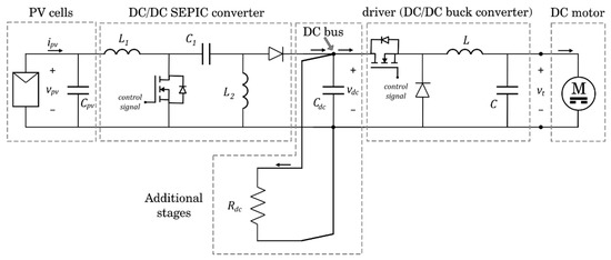
Figure 1.
Proposed system to regulate the angular speed of a DC motor powered by PV cells.
2.1. Modeling, Design and Control of the PV System
2.1.1. Modeling of the PV Cells
The equivalent electric circuit of the PV cells is shown in Figure 2. This is the most commonly used circuit in PV cell modeling and is known as the five-parameter model [53]. The circuit mainly comprises the following:

Figure 2.
Model of the PV cells.
ipv is the output current of the PV cells.
vpv is the output voltage of the PV cells.
IL = NpIph is the total photocurrent of the PV cells.
Np is the number of parallel PV cells.
Iph is the photocurrent of an individual PV cell.
I0 = NpIos is the saturation current of the diode.
Ios is the saturation current of an individual diode.
Rs is the series resistance of the PV cells.
Rp is the parallel resistance of the PV cells.
is the thermic voltage of the PV cells.
Ns is the number PV cells in series.
n is the emission coefficient.
kB is the Boltzmann constant with a value of .
is the electron charge with a value of .
T is the temperature of the PV cells, indirectly affected by the ambient temperature.
The current of the PV cells is given by:
Assuming that and , the following simplification of Equation (1) is made [54]:
2.1.2. P&O Algorithm Design on the SEPIC Converter
The operating principle of the P&O algorithm is based on the real-time voltage and current measurement of the PV cells to calculate the power and compare it iteratively with its previous value. Based on this comparison, the duty cycle of the converter is modified to track the MPP according to the higher power [20,55]. Figure 3 shows the P&O algorithm in the non-linear voltage vs. power curve of the PV cells using the SEPIC converter. Figure 3a shows the iterative MPP tracking process, where the algorithm’s behavior on the curve shows that its main drawback are oscillations around the MPP, involving variations in the DC bus. Figure 3b shows the basic cases of the algorithm, where ΔP and ΔV are the differences in the power and voltage of the PV cells with respect to their actual and previous values. As a result, the operating point on the curve can be to the left, the right, or exactly on the MPP. The duty cycle of the converter is modified to track the MPP depending on the location of the operating point on the curve.
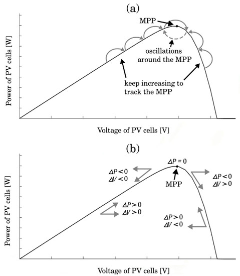
Figure 3.
P&O algorithm in the voltage versus power curve: (a) its behavior on the curve, (b) cases of the algorithm.
Figure 4 shows the flowchart of the P&O algorithm for the SEPIC converter based on the flowchart of the P&O algorithm, where ΔP is the power difference between the actual sample and the previous sample ; ΔV is the voltage difference between and the previous sample ; D is the duty cycle; and ΔD is the fixed increment to be added/subtracted to the duty cycle [55].

Figure 4.
Flowchart of the P&O algorithm for the SEPIC converter.
2.1.3. Modeling of the SEPIC Converter
The DC/DC SEPIC converter is used as the interface between the PV cells and DC bus, as shown in Figure 1. The dynamics of this converter and the PV cells are governed by Equation (3), where and are the current of the inductors and , respectively; is the current of the PV cells; , and are the voltages of the capacitors , and , respectively; is the impedance of the additional stages connected to the DC bus; and is the average control signal of the converter:
Equation (3) can be expressed as follows:
where:
The converter associated with the PV system is used to adjust the impedance seen by the PV cells. Therefore, in order to determine the relationship between the converter and this impedance, it is assumed that at a steady state the output voltage of the converter is:
If an energy balance is considered in the SEPIC converter , then the relationship between voltages and impedances of Equation (7) is obtained, where is the input impedance of the converter (also seen by the PV cells), and is the output impedance of the SEPIC converter (DC bus side):
By substituting Equation (6) into Equation (7), it is easy to deduce that:
It is observed from Equation (8) that the duty cycle of the SEPIC converter modifies the relationship between the impedances, which is the reason for using it as an interface to track the MPP. In addition, it is observed from Equation (6) that the converter also increases or decreases the input–output voltage ratio based on the duty cycle . As a result, if decreases/increases then also increases/decreases, though not proportionally, as shown in Equation (8). Similarly, will decrease/increase and will increase/decrease based on the voltage vs. current curve of the PV cells shown in Figure 5. The figure also shows that, when the impedance is higher, it enters the open-circuit voltage region, while it is in the short-circuit current region when the impedance tends to zero. The above shows that the rate of change in the duty cycle is always the opposite to the PV cells’ voltage rate, mathematically expressed as:
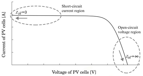
Figure 5.
Voltage vs. current curve of the PV cells.
2.1.4. Stability Proof of the PV System
The PV power is given by , and the power optimization is carried out by pushing the system to track a defined point as shown in Figure 6, resulting in:
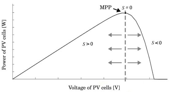
Figure 6.
Lyapunov function in the voltage vs. power curve of the PV cells.
Based on the Lyapunov function, the variable structure mode control requires that the following conditions be satisfied:
The Lyapunov function is proposed, as shown Equation (12), which considers the simplification of the current of the PV cells established in Equation (2):
From Equation (10) it is clear that when , the PV system reaches the maximum power point, and the system dynamics are analyzed in the other two states and . This is shown in Figure 6, where S < 0 corresponds to the right side of the MPP on the voltage vs. power curve, while corresponds to the left side of the same curve. Therefore, Equation (13) is obtained by partially deriving with respect to :
In the case of , cases ( and ) and ( and ) are covered, as shown in Figure 3b and Figure 6. This results in according to the P&O algorithm in Figure 4. Thus, from Equation (9) it follows that:
Replacing Equation (14) with Equation (13) results in:
In the case of , cases ( and ) and ( and ) are covered, as shown in Figure 3b and Figure 6. This results in according to the P&O algorithm in Figure 4. Equation (9) implies that the PV cells’ voltage increases and that:
Replacing Equation (16) into Equation (13) results in:
According to Equations (15) and (17), the system is globally stable since both conditions of Equation (11) are satisfied, and if then the system operates in the MPP according to Equation (10), which also makes it stable [54].
2.2. Modeling and ADRC Approach Design on the Motor Drive
Figure 7 shows the electrical diagram for regulating the angular speed of the DC motor, where is the average control signal of the ADRC approach, is the current of the inductor is the voltage of capacitor C (this voltage is the same as the motor terminals ), and are the inductance and resistance of the armature winding, respectively. , and represents the inertia, the coefficient of viscous friction, and the constant of the electromotive force of the DC motor, respectively. In addition, is the armature current, the electromotive force of the DC motor, is the angular speed and is the applied external torque. As the figure shows, is the variable power supply that includes variations in the DC bus caused by other stages connected to the bus, including the dynamics of the PV cells with the SEPIC converter, which in turn depend on environmental conditions.
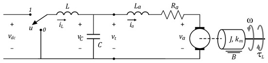
Figure 7.
Electrical diagram to regulate the angular speed of the DC motor using the ADRC approach.
The value of is considered constant only to simplify the mathematical model shown below, although it is clearly a variable term affected by environmental factors—the PV system and the DC bus itself. The aforementioned point represents a major advantage in reducing the design complexities of the control approach, and simplification is used because the ADRC approach is robust to changes in model parameters and the exact model of the system is not required. Moreover, it is observed in the results that the ADRC approach counteracts the effects of variations in the DC bus [50,56,57,58].
The average model of the system in state-space form is shown in Equation (18) and is only valid in the continuous conduction mode. The states are: , , , and . It is a fourth-order model () with a single input and a single output, and is linearly expressed in the typical form :
The operating points at which the system tends to operate under certain conditions of the variables are given by Equation (19), considering a constant steady-state value of voltages, currents and angular speed, i.e., from Equation (18). These operating points consider that is the desired angular speed of the DC motor, and is a constant steady-state applied torque on the motor shaft:
The dynamic design of the ADRC approach uses the differential flatness property, where the control inputs and all state variables are expressed in terms of the so-called flat outputs , where is the number of control signals. In this case, because the simplified system, as shown in Figure 7, only uses the control input . Therefore, the model of Equation (18) is expressed in terms of the flat output and its time derivatives by performing algebraic operations. For more details about differential flatness property, differentially flat systems and flat outputs, please consult references [59,60,61,62].
In this case, the proposed system is differentially flat if the system is shown to be controllable. Therefore, Equation (20) shows the Kalman controllability matrix , and the determinant of this matrix is shown in Equation (21). As a result, the system is differentially flat because it is also controllable:
The flat output of the system is determined using the inverse controllability matrix of Equation (20) and the state vector . The flat output is calculated using Equation (22), which results in the flat output being . However, the flat output is taken as the angular speed of the DC motor without loss of generality, i.e., [58,60]:
The state variables and the control signal of the model of Equation (18) are expressed in terms of the flat output and its time derivatives , , and . The result is shown in Equation (23):
The control signal of Equation (23) has several terms that are not so easily calculable or measurable. Therefore, Equation (24) shows a compact expression of this variable in terms of the highest-order derivative of the flat output and of a disturbance term . This term includes nonlinearities and internal and external disturbances in the system and is estimated by a GPI observer:
with
The design of the GPI observer to estimate the disturbance term begins with rearranging Equation (24) to express it in terms of , as shown in Equation (26). The basic idea of a GPI observer is to implement a linear observer that naturally incorporates integral actions regarding the output error. Similarly, for more details on GPI observers, please refer to [59,61,62]:
with
The next step consists of transforming Equation (26) as a pure integration chain as shown in Equation (28), where , and . These auxiliary variables express the equations based on the first derivative of each state variable to enable a better understanding of this integration chain:
Equation (29) shows the GPI observer, which consists of a reconstruction of (28) that includes a polynomial model in the time update of the perturbation in a natural and embedded form. The observer, which is similar to a Luenberger observer, uses the correcting terms to compensate for the estimated error. As a result, , and its four time derivatives are simultaneously estimated:
The system reconstruction error is shown in Equation (30), which is obtained by subtracting Equations (28) and (29), where , , and are the estimation errors of , , , and , respectively:
The system reconstruction error is reordered as:
In Equation (31), the following procedure is performed: the first four equations are derived and iteratively substituted with one another. As a result, the variable satisfies the following perturbed linear dynamics:
By applying the Laplace transform to Equation (32) with zero initial conditions, the characteristic polynomial of the tracking error is:
The choice of is set according to the characteristic polynomial of a desired, asymptotically and exponentially stable and unperturbed injected observation error dynamics [60,63]. For suitable strictly positive parameters , and , this polynomial is chosen as a fifth-order Hurwitz polynomial, as shown in Equation (34):
The values , and are chosen from the desired stability values using the pole placement method [32,59]. To facilitate the choice of these values, the recommended setting is or , and as half of , i.e., [60]. Subsequently, a sweep of is performed, starting with initial until a desirable behavior of the GPI observer is obtained:
In addition to the GPI observer, used to estimate the disturbance term, a second GPI observer is designed to estimate the load torque . This observer is not required by the ADRC approach and only performs the role of determining the torque caused by load and the external applied torque. The second GPI observer is designed in Equation (36), which is obtained from the angular speed equation of the dynamic model of Equation (18). Additionally, it is required to provide feedback of the armature current for proper operation:
The choice of , is also established according to the pole placement method using the following second-order Hurwitz polynomial:
where the values of and are given by Equation (38), with and :
With the GPI observer of Equation (29), the perturbation term is estimated, then the term of Equation (27) is estimated as shown in Equation (39):
Equation (39) implies that is now also known, so the control signal of Equation (24) is expressed as Equation (40):
An auxiliary controller is proposed to replace the higher-order derivative of the flat output, i.e., . This auxiliary controller is given by Equation (41) and performs the function of imposing closed-loop error dynamics behavior, as it is intended for , where is the angular reference angular speed of the DC motor [58,64]:
Substituting Equation (41) for Equation (40) results in:
By developing and comparing Equations (40) and (42), the following is obtained:
If the tracking error is , then , , and ; thus, the dynamics of the closed loop tracking error satisfies:
by applying the Laplace transform with initial conditions equal to zero:
As a result, the characteristic polynomial of the tracking error dynamics is obtained as:
where the gains of this characteristic polynomial must be chosen in such a way that their roots are located in the left semiplane of the complex plane. For this reason, a fourth-order Hurwitz polynomial is proposed to impose the desired dynamic—:
The values of the auxiliary controller coefficients are obtained in Equation (48), where and . The pole placement method is also used as with the GPI observers to facilitate the choice of these values. In this case, the recommendation is to set = 0.707 or = 0.9, while must be selected between five and ten times less than the [60]. It is then corroborated whether the angular speed behavior of the DC motor satisfies requirements such as maximum overshoot or settling time in accordance with the system requirements:
Finally, this study is only concerned with angular speed regulation without trajectory tracking, which implies: . Therefore, Equation (49) shows the simplified auxiliary controller of Equation (41), which also considers the time derivatives of the flat output estimated by the GPI observer of Equation (29):
The final form of the control law for the regulation of the DC motor’s angular speed by means of the ADRC approach is expressed in Equation (50):
The FPGA implementation requires discretization of the equations. The simplest form is the recursive Euler approximation method given by Equations (51) and (52), where is the approximate derivative; and are the outputs of the current and previous samples, respectively. is the sampling period between each sample. The reason for selecting this approach is that it is easier to implement than the forward or trapezoidal Euler’s methods, since it only requires the present and past values of the variable to be discretized. In addition, the results below show that this method is sufficient:
Then, the discretization of the GPI observer to estimate the disturbance term in Equation (29) is:
The discretization of the second GPI observer used to estimate the load torque in Equation (36) is:
and the discretization of the auxiliary controller in Equation (49) is:
Finally, the discretization of the control law in Equation (50) is:
Table 1 summarizes the equations required to control the entire system, which were discretized if necessary. These equations are implemented in the Nexys 4 development board with an Artix–7 FPGA in Section 3.

Table 1.
Equations required to control the entire system.
3. FPGA Architecture and Hardware Implementation
Figure 8 shows the block diagram of the proposed system’s organization. The hardware includes the PV cells, two electronic converters, the DC motor, a dynamometer to measure the angular speed and apply a load torque to the motor shaft, voltage and current sensors, analogic-to-digital converters (ADCs) to digitize the sensor signals, and the PWM control signal conditioning stage that uses transistor gate drivers and the Nexys 4 development board with an FPGA from the Artix-7 family. The software includes digitized signals in a 32-bit floating-point representation using the IEEE 754–1985 standard, synthesis of the P&O algorithm and the ADRC approach, including the GPI observer, auxiliary controller and linear controller, and the PWM generation to convert the average signal into a switched signal. The software takes advantage of the FPGA’s concurrency to simultaneously evaluate the different process, which is the main reason for choosing this digital device. Further details on FPGA architecture and the implementation of the experimental platform are presented below.
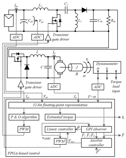
Figure 8.
Block diagram of the proposed system.
3.1. FPGA Architecture
The FPGA architecture design uses the VHDL hardware description language and the Xilinx System Generator tool in a hierarchical and modular manner with a top-down methodology. The operating frequency is, which is equivalent to a period of . In addition, a clock frequency of is used for the ADC, where the time for digitizing a data is:
Figure 8 shows that the resulting FPGA architecture is composed of six main modules: the P&O algorithm module, two GPI observer modules, the auxiliary controller module, the linear controller module, and the PWM module.
Figure 9 shows the implementation of a P&O algorithm module based on the flowchart in Figure 4. The structure of this module was designed to take advantage of the independence between its elements and the concurrent paradigm that an FPGA offers. The implementation of Figure 9 has the following considerations:

Figure 9.
Implementation of P&O algorithm module.
- The current Ipv[k] and the voltage Vpv[k] are measured in the PV cells. A throughput rate of 1 KSPS is defined, considering that the dynamics of the PV cells is relatively slow. Therefore, the sampling period is Ts,P&O = 1 ms.
- The power of the current sample is then calculated. The previous power is also calculated using the previous values of current and voltage stored in registers.
- The power and voltage differences are calculated in order to proceed to the decision stage, i.e., and .
- The decision stage of the P&O algorithm is carried out through the multiplexers where it is compared if ΔP = 0, ΔP > 0 and ΔV > 0. The output value of this process is one of the three possible fixed values {–1, 0, 1}.
- The output value multiplies ΔD = 0.005 to obtain one of three values {−ΔD, 0, ΔD}. The result is added to the duty cycle of the previous sample and a new iteration is generated to modify the voltage’s behavior versus the power curve of the PV cells, i.e., .
- As a result, there is an average continuous control signal D[k] ∈ [0,1].
- The synthesis tool shows that the propagation delay generated by this module is:
In the case of ADRC approach used to control the motor drive, Figure 10, Figure 11, Figure 12 and Figure 13 show the FPGA architecture of the equations in Table 1 for the DC motor angular speed control. This approach needs to measure the flat output , as shown in Figure 10, Figure 11 and Figure 12. In addition, the second GPI observer also needs to measure the armature current of the DC motor for estimating the torque in the shaft, as shown in Figure 11. These signals are monitored with a dynamometer, as well as a current sensor, and are discretized by the ADC. In this case, the sampling period is , which is a much shorter period than the P&O algorithm module because the DC motor dynamics are faster than the PV dynamics. The FPGA architecture consists of addition, subtraction and multiplication operations that are concurrently performed with non-pipeline stages in a 32-bit floating point arithmetic. The propagation delay of the multipliers, adders and subtractors are , and , according to the synthesis tool. In some cases, there are registers to synchronize all the necessary input signals, where its propagation delay is .
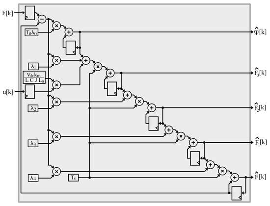
Figure 10.
Implementation of the GPI observer module that estimates the disturbances.
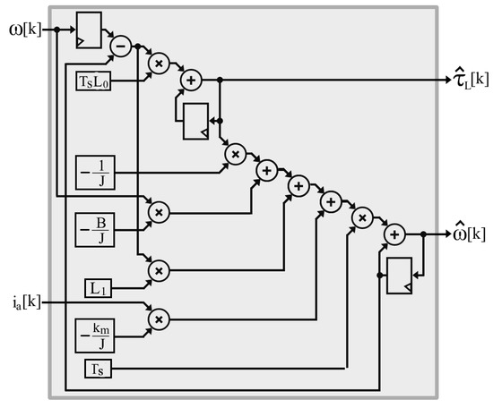
Figure 11.
Implementation of the GPI observer module that estimates the load torque.
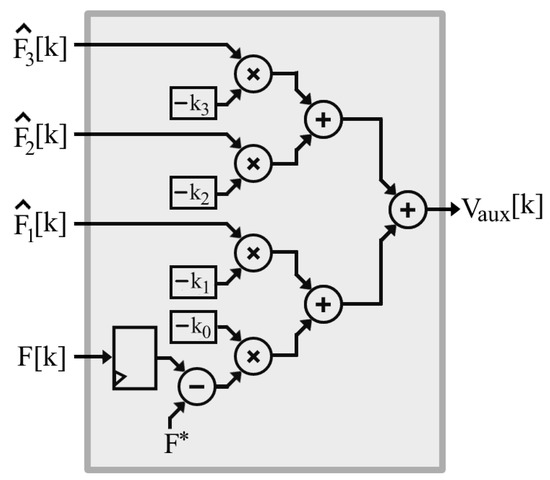
Figure 12.
Implementation of the auxiliary controller module.
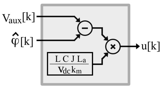
Figure 13.
Implementation of the final linear control law module.
Figure 10 shows the implementation of the GPI observer module that estimates the disturbances given by Equation (53). As a result, and the flat output and their first three temporal derivatives are simultaneously estimated. As previously mentioned, this module was designed in a concurrent manner to take advantage of the independence of its different elements and minimize propagation time. The propagation delay generated by this module, considering that the signal has the largest number of mutually dependent operations, results in a propagation delay of:
Figure 11 shows the implementation of the second GPI observer module, which estimates the load torque given by Equation (54). The propagation delay of this module is defined by Equation (60), considering that is the variable with the largest number of mutually dependent operations:
Figure 12 shows the implementation of the auxiliary controller module given by Equation (55). In this module, only the input is synchronized through the register, as the other signals are directly connected from the output of the GPI observer module from Figure 10. It can also be noted that the desired angular speed is set in this module. As a result, the propagation delay is:
Figure 13 shows the implementation of the final linear control law module given by Equation (56). This module is the simplest element of ADRC approach, which does not include input registers as all signals are directly connected from the output of the GPI observer module and the auxiliary controller module from Figure 10 and Figure 12, respectively. The propagation delay of this module is:
Figure 14 shows the implementation of an individual PWM module. The PWM module transforms the average control of the P&O algorithm module and the final linear control law module , from Figure 9 and Figure 13, respectively, into switched signals for the proper operation of the DC/DC converters. The module consists of fast PWM, where the average signal is compared to a triangular signal generated from an 11-bit counter. The PWM module includes a submodule that converts it into an 11-bit unsigned binary format, since the average signal is represented by a 32-bit floating point arithmetic. The PWM frequency is defined by Equation (63), where the frequency of the clock counter is , and the count ranges from 0 to 1999.
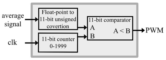
Figure 14.
Implementation of an individual PWM module.
As a result, the propagation delay of the PWM module is:
Figure 15 shows the timing diagram of the FPGA architecture. There are three main independent parts running in parallel: the P&O algorithm, the load torque GPI observer, and the ADRC approach. The figure shows the times for each part, where the period required for digitizing data is the component that requires the most time. As a result, the ADRC approach takes the longest time to complete, although the time is almost half of the minimum value established as the sampling time. This is because the architecture takes advantage of the concurrence, as if a sequential device were used; therefore, the time would certainly be longer than the set sampling time. If this were to occur, it would lead to problems of signal collision.
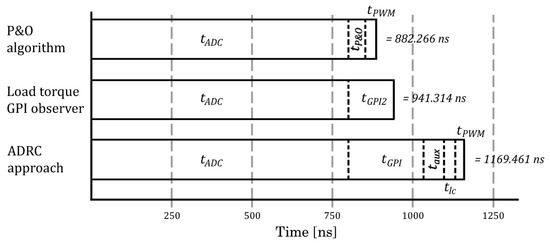
Figure 15.
Timing diagram of the software.
Finally, Table 2 summarizes the device utilization reports with the main resources used by the FPGA and shown in Figure 9, Figure 10, Figure 11, Figure 12, Figure 13 and Figure 14, according to the synthesis tool. Embedded multipliers (DSP48E1s) are the most commonly used resource (92%), as floating-point arithmetic operations are performed by these resources. Based on these data, the FPGA resources are sufficient for all the software used.
Table 2.
Device utilization reports used by the Artix–7 FPGA.
Simulation and implementation projects are available as Supplementary Material. This material is openly available in FigShare at https://doi.org/10.6084/m9.figshare.20405913, reference number [65]. The simulation project includes a Matlab/Simulink simulation of the system: photovoltaic cells + SEPIC converter + Buck converter + DC motor. The simulation uses XSG blocks for the control stage and Simulink blocks for the power stage. The implementation project includes the whole control part of the system to be implemented on the Nexys 4 development board (see Figure 9, Figure 10, Figure 11, Figure 12, Figure 13 and Figure 14). In addition, three examples of ISE design projects created with different speed references are shown.
3.2. Hardware Implementation
According to Figure 1 and Figure 8, the hardware employed in this system consists of PV cells, the SEPIC converter, the DC bus, a resistor in the DC bus used as variable loads, the DC/DC buck converter and the DC motor. With regard to the PV cells, Table 3 shows the nominal values of the Eco Green Energy EGE-260P-60 solar panel used under standard test conditions (STC) and normal operating cell temperature (NOCT).
Table 3.
Nominal values of the solar panel Eco Green Energy EGE-260P-60.
The nominal values used in the SEPIC converter are:
, , .
The nominal values used in the DC bus and the motor drive are:
,
, .
The nominal DC motor parameters are:
, , , .
with the following electromagnetic design parameters:
, La = 0.039 H, , , .
Experimental tests showed that the efficiency of the SEPIC and buck converters are 90% and 91%, respectively. However, it should be clear that the motor has a load-dependent power consumption, so not all of the power from the PV cells is required by the DC motor. In fact, it is more important that the energy harvested from the PV system is the energy needed to feed the DC motor and the additional stages. Therefore, the efficiencies are relatively sufficient for the purpose of the system, although better designed converters would be preferable in order to increase the efficiency of the system.
In addition, the system has the following additional hardware:
- Lem HX-15-P hall effect current sensor for measuring the PV cells and DC motor currents.
- A resistive network to measure the PV cells voltage.
- AD7476A ADC with a resolution of 12 bits. This is used to digitize the voltage and current of the PV cells, the current and the speed of the DC motor.
- The IRF640 MOSFET and the U15A40 diode are the semiconductor devices in each converter.
- To increase the switch’s reliability, a resistor–capacitor–diode snubber circuit is used in each converter, where the resistance and capacitor values for the SEPIC and buck converter are 15 Ω/68 nF and 47 Ω/22 nF, respectively.
- Conditioning of the PWM signals to properly switch the power converters, which consists of an isolation by means of an optocoupler (PC923 CI) and a power driver (IRF2117 CI).
Figure 16 shows the Eco Green Energy EGE-260P-60 solar panel that was used, with a N142° orientation basis. The figure shows three solar panels but only one is used which is marked in a box. The structure supporting the PV cells has a minimum height of 0.2 m and a maximum height of 0.4 m, so that it is ventilated for a better performance. Therefore, the inclination angle of the solar panel is 20° from its lowest part. The experimental platform is shown in Figure 17, where the connections consist of the solar panel voltage input, as shown in Figure 16, to a PCB for measuring its voltage and current. The output of this PCB is then connected to the SEPIC converter, which in turn is connected to a resistor array Rdc and the motor drive. The motor drive is the DC/DC buck converter, which is connected to the DC motor at the output. In the motor drive’s PCB, the current circulating in the DC motor armature winding is measured. The DC motor is connected to the dynamometer through a toothed belt, so the dynamometer is used for measuring the angular speed and applying the torque on the shaft. In addition, the Nexys 4 development board connects to the ADCs to acquire the different signals being measured. The board also interfaces with the PWM signal conditioning stage before being routed to the power electronic converters.
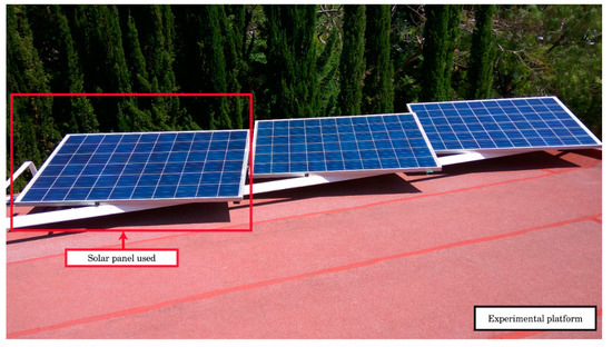
Figure 16.
Eco Green Energy EGE-260P-60 solar panel used.
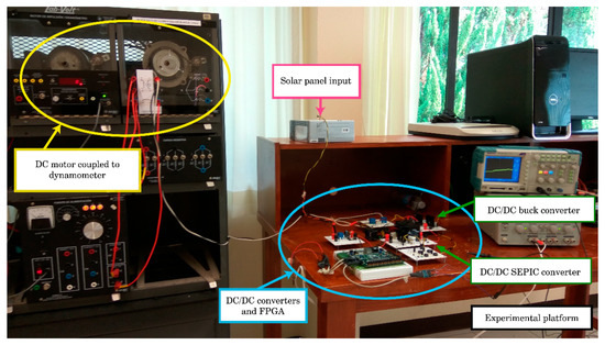
Figure 17.
Experimental prototype of the PV system.
4. Experimental Results
Figure 18 shows the behavior of the incident irradiance from 8:00 a.m. to 7:00 p.m. in the second half of August 2020 in the city of Huajuapan de León, Oaxaca, Mexico (17°48′14″ N, 97°46′33″ W). The behavior of the irradiance resembles a parabolic cylinder, where the highest levels are obtained between 1:00 p.m. and 2:30 p.m., while the lowest levels occur at dawn and sunset. In addition, the irradiance never remains constant, which in turn implies that the maximum power point of the solar panel also varies during the day.
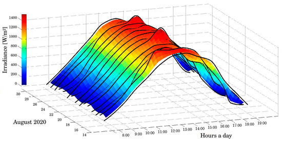
Figure 18.
Experimental test irradiance.
4.1. Maximum Power Point Tracking of the PV Cells
The first test focuses on MPP tracking using the P&O algorithm, as shown in Figure 19. In this test, a constant duty cycle of 0.5 is initially used in the SEPIC converter with the following irradiances , considering that the PV cells are not in the MPP. At t = 0.4 s, the P&O algorithm is enabled in the PV system to track the MPP. Figure 19a shows the behavior of the duty cycle of the SEPIC converter, where it is observed that in all cases, the value of the duty cycle is modified to track the MPP. In addition, the duty cycle is higher if the irradiance also increases. Figure 19b shows the output voltage of the SEPIC converter, which is the same as the DC bus vdc. This figure shows that the SEPIC converter boost the input voltage of the PV cells, according to the duty cycle of the P&O algorithm. Figure 19c shows the voltage of the PV cells, where it is observed that the voltage decreases when operating at MPP. Figure 19d shows the current of the PV cells, where it is observed that the current significantly increases when the system operates at MPP. According to the voltage and current behavior shown in Figure 19c,d, it is noted that the initial constant duty cycle of 0.5 operates on the open-circuit voltage-side of the PV cells (see Figure 3a and Figure 5). Figure 19e shows the power of the PV cells, which is a multiplication of its voltage and current. The results show the importance of MPP tracking since the constant duty cycle only obtains an approximate PV cell power of 20 W, while the power varies using the P&O algorithm depending on environmental conditions, although it is always higher. In the best case scenario, the power output of the PV cells under the same conditions is 10.5 times higher (considering ), and in the worst case scenario, it is 5.8 times higher (considering ).
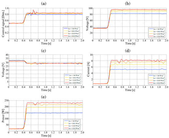
Figure 19.
MPP tracking: (a) P&O algorithm signal control, (b) DC bus voltage, (c) PV cells voltage, (d) PV cells current, and (e) PV cells power.
Irradiance greatly influences the behavior of the control signal, voltage, current and power of the PV cells in the MPP. Therefore, this test consisted of obtaining the MPP of the PV cells under different irradiance levels to measure the values of the different variables involved. Figure 20 shows the behavior of these signals as a function of the incident irradiance to appreciate the dependence. The figure shows the experimental values obtained together with their curve fitting, considering a second-degree polynomial function. In Figure 20a, the behavior of the control signal in the P&O algorithm’s MPP is shown, which tends to increase when the irradiance also increases. Figure 20b shows that the DC bus vdc also tends to be higher as the irradiance increases, mainly because the duty cycle increases. The opposite occurs in the case of the PV cells voltage in the MPP, since Figure 20c shows that when the irradiance is greater, this leads to a temperature increase in the PV cells, and then the Vmpp decreases. Figure 20d shows that the current in the MPP also tends to increase according to the irradiance levels, with the irradiance having a much greater influence on the current obtained, and consequently, an influence on the power of the PV cells. Finally, Figure 20e shows that the maximum power of the PV cells also increases as the irradiance increases. For example, when there is a maximum power of approximately 135 W with an irradiance of 700 W/m2, the maximum power is approximately 230 W for an irradiance of 1260 W/m2, i.e., a difference of 95 W. If transferred to that shown in Figure 18, this would mean that the maximum power at 9:00 h under optimal environmental conditions would be at least 95 W, and would be better during the day until reaching the MPP at about 13:30 h.
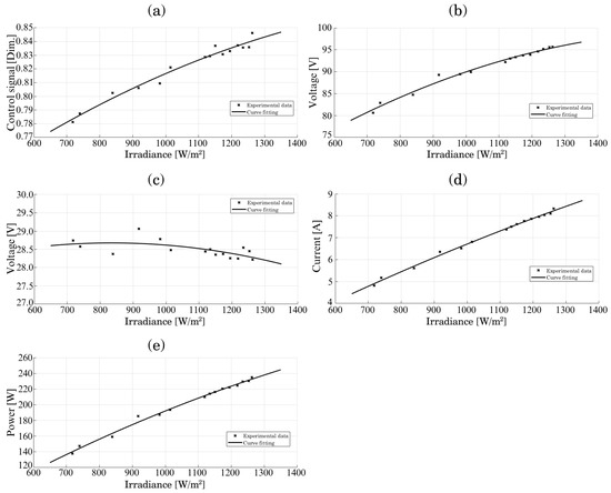
Figure 20.
PV system variables behavioral in the MPP: (a) P&O algorithm signal control, (b) DC bus voltage, (c) PV cells voltage, (d) PV cells current, and (e) PV cells power.
Based on the results, the P&O algorithm is sufficient for the purposes of this system. It can also be noted from the results that the maximum power is never equal to the values in Table 3 since they do not operate under the STC or NOCT conditions. In addition, it is shown that PV cells are not a power source that provide a constant voltage/current; its behavior is non-linear and mainly depends on the irradiance. Therefore, this should be taken into consideration and verified in the power design requirements of any system or, in any case, an oversized PV system.
4.2. Effects in the MPP of PV Cells Due the Connection of the DC Motor
Figure 19 and Figure 20 focus on the variables related to the PV cells and its corresponding converter to MPP tracking under different irradiance levels. This section aims to observe the performance of the whole system due to the connection of the DC motor. Therefore, Figure 21 shows the behavior of an experimental test with a particular irradiance Irr = 1186 W/m2, where the voltage, current and power in the MPP in the specific irradiance are: , and , respectively. The figure includes the following four stages:
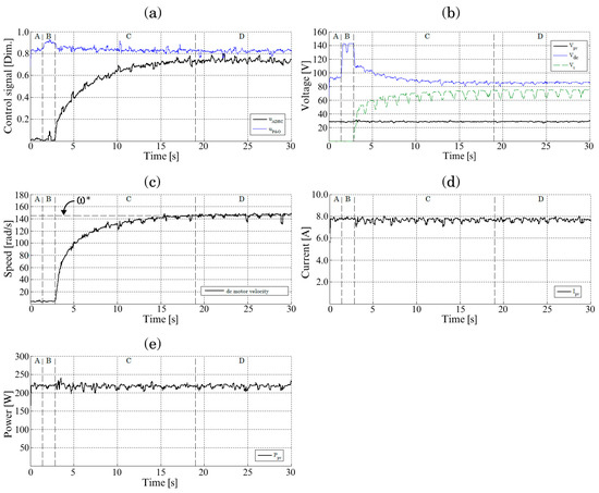
Figure 21.
PV system behavioral with (a) P&O algorithm and ADRC approach control signals; (b) PV cells, DC bus and DC motor terminals voltages; (c) DC motor angular speed (d) PV cells current; and (e) PV cells power.
- Stage (A): The PV cells are at MPP, which occurs after enabling the P&O algorithm, as shown in Figure 19. The resistor Rdc has a value of 54 Ω, which emulates the connection of other loads. In addition, the ADRC control signal is disabled, and the DC motor has a speed of 0 rad/s.
- Stage (B): At t = 1.40 s, there is a change in the resistance of the DC bus Rdc, from 54 Ω to 155 Ω. This change in the load causes variations in the DC bus and is a disturbance that the ADRC approach must counteract.
- Stage (C): At t = 2.85 s, the ADRC signal is enabled, causing the operation of the driver and starting the DC motor. At this time, the drive impedance varies, so the ADRC approach must also counteract this disturbance.
- Stage (D): At t = 19 s, the DC motor angular speed reaches the steady state, and F* = ω* = 145 rad/s. Therefore, the PV cells are at MPP, and the DC motor has the desired angular speed.
Figure 21a shows the evolution of the control signals during the four stages of the P&O algorithm and the ADRC approach. Originally, the steady-state value of the P&O algorithm control signal is 0.83 for stage A, but it reaches 0.90 for stage B and 0.82 for stage D. It should be noted that, although the irradiance is the same during the four stages, the control signal varies in order to track the MPP. The control signal of the ADRC approach is different to zero when enabled at stage C and reaches a steady-state value of 0.77 at stage D. At the beginning of stage C, the motor starts to rotate and the evolution of the motor’s angular speed is shown in Figure 21b. This figure shows that the desired velocity of 145 rad/s is reached during stage D.
Figure 21c shows the voltage behavior of the PV cells Vpv, the DC bus Vdc, and the voltage in the terminals of the DC motor Vt. In the case of Vpv, this remains at an average value of 28.40 V at all stages, which is a voltage at the MPP for the specified irradiance. Vt has a value greater than zero up to stage C because at this point the ADRC approach is enabled. vdc increases from 92.50 V in stage A to 142.50 V in stage B, but drastically decreases when the DC motor starts operating. All of these changes are caused by impedance changes in the DC bus. The changes in vdc are due to the P&O algorithm tracking the MPP, which depends on the impedance reflected at the input of the SEPIC converter, affected by Rdc and the impedance of the DC motor drive.
Figure 21d,e show the current Ipv and power Ppv of the PV cells, respectively. As in the case with Vpv, both Ipv and Ppv present minimal variations, maintaining the average current and power of 7.770 A and 220.67 W delivered by the PV cells. These values are maintained despite the changes in the DC bus, in particular the change in Rdc and the connection of the DC motor drive. Based on the above, the effectiveness of the P&O algorithm to track the MPP is demonstrated and is sufficient for this purpose. In addition, the maximum power of the PV cells Pmpp depends on their respective incident irradiance and temperature, and not on the variations in the load or the DC bus, as shown by the different stages presented.
4.3. DC Motor Angular Speed Regulation
This section focuses on the DC motor angular speed regulation results, which are equivalent to stages C and D of Figure 21. Therefore, the PV system is assumed at MPP to occur during stage B. In the following test, the PV system has an incident irradiance of Irr = 1263 W/m2 with an applied load torque of to the DC motor shaft. In addition, the PV cells are in the MPP with a . The GPI observer, auxiliary controller and torque estimator gains are shown in Table 4. It is worth mentioning that, for all the tests and environmental conditions the same gains of the GPI observers of Equations (35) and (38), and the auxiliary controller of Equation (48) were used.
Table 4.
GPI observer and auxiliary controller gains.
Figure 22a shows the soft evolution of the average ADRC signal, reaching an approximate steady-state value of , with an establishing time of s. Figure 22b shows the DC motor angular speed, which corresponds to the reference value of during the establishing time. Figure 22c shows the angular speed error between the desired speed and motor shaft speed, where there is a maximum error of which is equivalent to a maximum error of . The integral absolute error (IAE) given by Equation (65) is used to quantitatively evaluate the performance of the ADRC approach. Therefore, Figure 22d shows the behavior of the IAE of the ADRC approach, which presents a significant value given that it is a regulating study and not a trajectory tracking. This implies that a relatively large error occurs during the motor start-up, where it takes approximately to reach the desired angular speed.
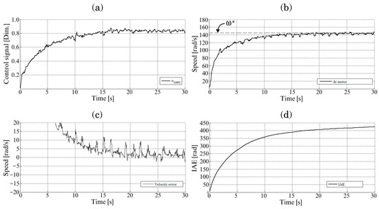
Figure 22.
DC motor angular speed regulation: (a) ADRC approach control signal, (b) DC motor angular speed, (c) speed regulation error, and (d) IAE of angular speed.
It should be noted in Figure 21 and Figure 22 that the desired angular velocity is obtained despite the different variations in the DC bus and PV cells as it counteracts them. Proper control performance depends on an accurate estimation of system disturbances, which is obtained through a GPI observer. Therefore, Figure 23a shows the estimation of the disturbance from Equation (53), which has a steady-state value of −3.3 × 10¹¹ rad/s5. This estimated term is counteracted in the linear controller of Equation (56), which is the reason for the effectiveness of the ADRC approach. Figure 23b shows the comparison between the output and the estimated angular speed from Equation (53). The output of this observer is considered functional since it presents similar values of estimation with a real speed, which gives certainty to the perturbation estimation. Figure 23c shows the estimation error between the estimated speed and motor shaft speed, which is approximately zero. Figure 23d shows the histogram of the estimation error in conjunction with its normal distribution, where the statistical summary is given by Table 5. The data of Figure 23d and Table 5 show that the estimation error is centered around zero, where the measures of location do not exceed a maximum error of , although the maximum error is greater than 10 rad/s. Finally, Figure 23e shows the estimated torque given by Equation (54), which is the sum of the applied torque and the torque generated by the friction of the toothed belt that connects the DC motor to the dynamometer. As a result, the value of the estimated torque is , which is consistent with the applied torque. Based on Figure 21, Figure 22 and Figure 23, the effectiveness of the GPI observers is demonstrated and can also counteract undesired effects in order to regulate the speed to the desired value. It is extremely important to note that if the estimator fails, then the desired speed cannot be reached.
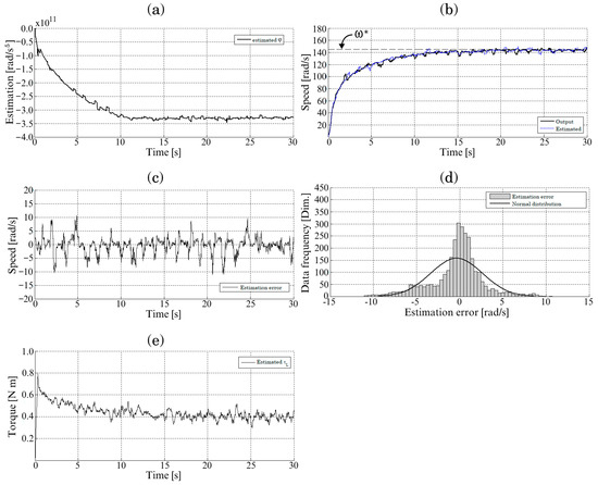
Figure 23.
GPI observers signals: (a) estimation of disturbances , (b) output and estimated angular speed, (c) estimation error, (d) histogram of estimation error, and (e) torque load estimation.
Table 5.
Summary statistics of GPI observer that estimate the disturbances.
4.4. Effects of Irradiance Variations on the Angular Speed of the DC Motor
It is shown in Figure 19, Figure 20 and Figure 21 that the PV cells are a non-linear power supply that depend on the incident irradiance. However, the angular speed of the DC motor also indirectly depends on this independent variable since the motor consumes a certain amount of Pmot = 160 W power because of the tests carried out. Therefore, this power must at least be supplied by the PV cells, an example being the irradiance used in the test of Figure 21, which was Irr = 1186 W/m2, while the test in Figure 22, it was Irr = 1263 W/m2. The PV system consequently requires a minimum irradiance to satisfy the power demand of the load, in this case, the motor drive and resistance Rdc. Figure 24 shows the effect of irradiance variations on different signals related to the angular speed control of the DC motor to determine the minimum operating conditions for regulating the speed to the desired value. Figure 24a shows the DC motor input voltage, which varies from 70 V to 85 V, with an irradiance of 975 W/m2 from 1240 W/m2, respectively. Figure 24b shows the ADRC approach control signal, and Figure 24c shows the DC motor angular speed. As can be seen, if the irradiance is less than 975 W/m2, then the desired angular speed of 145 rad/s cannot be reached. Based on the above, it is established that the minimum irradiance for correctly regulating the angular speed in 145 rad/s of the DC motor must be at least 1000 W/m2 under the design aspects used in the system. The previously mentioned data do not imply that the ADRC approach is not sufficiently robust to changes of irradiance, as this approach was able to regulate the angular speed of the DC motor to the desired level under different test scenarios. However, what is determined is the minimum level of irradiance required for proper operation, when due to an uncontrolled physical limitation, the PV cells do not supply enough energy to the load, and thus cannot be regulated to the desired angular speed.

Figure 24.
Irradiance variation effects in: (a) DC motor input voltage, (b) ADRC signal control, and (c) DC motor speed.
5. Conclusions
A system for controlling the speed of a DC motor powered by solar PV energy is presented in this paper. An initial problem appears because the PV cells are a non-linear power supply. The results from Figure 20 show that the maximum energy harvesting from PV cells is especially dependent on the incident irradiance, since a higher irradiance increased the maximum amount of energy. For this reason, a SEPIC converter and the P&O algorithm were used to track the MPP, which implied transferring the maximum power from the PV cells to the DC bus.
The results from Figure 19, Figure 20 and Figure 21 and Figure 24 show the importance of MPP tracking. In particular, Figure 19 shows that the energy harvested from PV cells is five to ten times higher when the P&O algorithm is used. The P&O algorithm was appropriate for this purpose even though there are better techniques because it is a relatively small system that had no problems with the partial shading condition.
However, the P&O algorithm and many MPPT techniques only harvest the maximum energy from the PV cells. This caused variables such as voltage and current to vary in achieving their objective, resulting in a variable source for the DC motor. For this reason, the ADRC approach was used to counteract the effects of these and other variations.
Figure 21, Figure 22 and Figure 23 show that the ADRC approach regulated the angular speed of the DC motor to a desired value under varying conditions. In particular, Figure 21 and Figure 23 show that the control approach estimated and canceled the effects of variations in environmental conditions, the photovoltaic system, the DC bus, and the load changes in order to regulate the DC motor speed.
In addition, this paper shows the complete design of the FPGA architecture to implement the P&O algorithm and the ADRC approach. The architecture design was developed in a hierarchical and modular manner using a top-down methodology. It is important to mention that this material is openly available. The designed architecture could reduce software execution times through the simultaneous use of methods. In this sense, Figure 15 shows that three main tasks were performed in parallel, and even within these tasks, other operations are performed in parallel. As a result, the execution time of the whole control approach corresponds to the execution time of the ADRC approach since only the longest execution time among all tasks is considered. Figure 15 shows that this time is approximately 1.170 µs, much less than the established sampling time of 2 µs.
Finally, Figure 24 shows that the angular speed also depends on the level of irradiance in this system. In this case, a minimum irradiance of 1000 W/m2 is required according to the experimentation for a desired angular speed of 145 rad/s, with a load torque of τL = 0.40 Nm. This is an important consideration that must be taken into account in the design of systems using this type of energy. Based on the above, future research should focus on the design of a more complete system based on distributed generation, where the PV system has a stage that transfers energy to the grid when the energy generated is greater than the energy used. This configuration allows the DC motor to simultaneously use and transfer energy to the grid when necessary. In addition, the dissipating load Rdc is replaced by a more practical stage.
Author Contributions
Conceptualization, E.G.-R. (Esteban Guerrero-Ramirez) and M.A.C.-O.; methodology, E.G.-R. (Esteban Guerrero-Ramirez) and A.M.-B.; software, E.G.-R. (Esteban Guerrero-Ramirez), A.M.-B. and E.G.-R. (Enrique Guzman-Ramirez); validation, G.G.-R., J.L.B.-A. and M.A.-M.; formal analysis, E.G.-R. (Esteban Guerrero-Ramirez), M.A.C.-O. and G.G.-R.; investigation, A.M.-B., J.L.B.-A. and E.G.-R. (Enrique Guzman-Ramirez); resources, E.G.-R. (Enrique Guzman-Ramirez) and M.A.-M.; data curation, A.M.-B.; writing—original draft preparation, E.G.-R. (Esteban Guerrero-Ramirez) and A.M.-B.; writing—review and editing, M.A.C.-O., G.G.-R., E.G.-R. (Enrique Guzman-Ramirez), J.L.B.-A. and M.A.-M.; project administration, E.G.-R. (Esteban Guerrero-Ramirez). All authors have read and agreed to the published version of the manuscript.
Funding
This research has been funded in part by TecNM/Cenidet. Project number: 63n4up (14877.22-P).
Institutional Review Board Statement
Not applicable.
Informed Consent Statement
Not applicable.
Data Availability Statement
Not applicable.
Conflicts of Interest
The authors declare no conflict of interest.
References
- Rabaia, M.K.H.; Abdelkareem, M.A.; Sayed, E.T.; Elsaid, K.; Chae, K.-J.; Wilberforce, T.; Olabi, A. Environmental impacts of solar energy systems: A review. Sci. Total Environ. 2021, 754, 141989. [Google Scholar]
- Sampaio, P.G.V.; González, M.O.A. Photovoltaic solar energy: Conceptual framework. Renew. Sustain. Energy Rev. 2017, 74, 590–601. [Google Scholar] [CrossRef]
- Bose, B.K. Global Energy Scenario and Impact of Power Electronics in 21st Century. IEEE Trans. Ind. Electron. 2013, 60, 2638–2651. [Google Scholar] [CrossRef]
- Rahman, S.; Meraj, M.; Iqbal, A.; Tariq, M.; Maswood, A.I.; Ben-Brahim, L.; Al-Ammari, R. Design and Implementation of Cascaded Multilevel qZSI Powered Single-Phase Induction Motor for Isolated Grid Water Pump Application. IEEE Trans. Ind. Appl. 2019, 56, 1907–1917. [Google Scholar] [CrossRef]
- De Almeida, A.; Fong, J.; Brunner, C.U.; Werle, R.; Van Werkhoven, M. New technology trends and policy needs in energy efficient motor systems–A major opportunity for energy and carbon savings. Renew Sustain. Energy Rev. 2019, 115, 109384. [Google Scholar] [CrossRef]
- Kabir, E.; Kumar, P.; Kumar, S.; Adelodun, A.A.; Kim, K.-H. Solar energy: Potential and future prospects. Renew. Sustain. Energy Rev. 2018, 82, 894–900. [Google Scholar] [CrossRef]
- Wang, J.; O’Donnell, J.; Brandt, A.R. Potential solar energy use in the global petroleum sector. Energy 2017, 118, 884–892. [Google Scholar] [CrossRef]
- Hernández-Callejo, L.; Gallardo-Saavedra, S.; Alonso-Gómez, V. A review of photovoltaic systems: Design, operation and maintenance. Sol. Energy 2019, 188, 426–440. [Google Scholar] [CrossRef]
- Obeidat, F. A comprehensive review of future photovoltaic systems. Sol. Energy 2018, 163, 545–551. [Google Scholar] [CrossRef]
- Algarín, C.R.; Giraldo, J.T.; Álvarez, O.R. Fuzzy Logic Based MPPT Controller for a PV System. Energies 2017, 10, 2036. [Google Scholar] [CrossRef]
- Rezk, H.; Aly, M.; Al-Dhaifallah, M.; Shoyama, M. Design and Hardware Implementation of New Adaptive Fuzzy Logic-Based MPPT Control Method for Photovoltaic Applications. IEEE Access 2019, 7, 106427–106438. [Google Scholar] [CrossRef]
- Jiang, L.L.; Maskell, D.L.; Patra, J.C. A novel ant colony optimization-based maximum power point tracking for photovoltaic systems under partially shaded conditions. Energy Build. 2013, 58, 227–236. [Google Scholar] [CrossRef]
- Titri, S.; Larbes, C.; Toumi, K.Y.; Benatchba, K. A new MPPT controller based on the Ant colony optimization algorithm for Photovoltaic systems under partial shading conditions. Appl. Soft Comput. 2017, 58, 465–479. [Google Scholar] [CrossRef]
- Tey, K.S.; Mekhilef, S.; Seyedmahmoudian, M.; Horan, B.; Oo, A.T.; Stojcevski, A. Improved Differential Evolution-Based MPPT Algorithm Using SEPIC for PV Systems Under Partial Shading Conditions and Load Variation. IEEE Trans. Ind. Inform. 2018, 14, 4322–4333. [Google Scholar] [CrossRef]
- Aouchiche, N.; Aitcheikh, M.; Becherif, M.; Ebrahim, M. AI-based global MPPT for partial shaded grid connected PV plant via MFO approach. Sol. Energy 2018, 171, 593–603. [Google Scholar] [CrossRef]
- Shi, J.-Y.; Zhang, D.-Y.; Xue, F.; Li, Y.-J.; Qiao, W.; Yang, W.-J.; Xu, Y.-M.; Yang, T. Moth-Flame Optimization-Based Maximum Power Point Tracking for Photovoltaic Systems Under Partial Shading Conditions. J. Power Electron. 2019, 19, 1248–1258. [Google Scholar]
- Messalti, S.; Harrag, A.E.; Loukriz, A. A new variable step size neural networks MPPT controller: Review, simulation and hardware implementation. Renew. Sustain. Energy Rev. 2017, 68, 221–233. [Google Scholar] [CrossRef]
- Elkholy, M.M.; Fathy, A. Optimization of a PV fed water pumping system without storage based on teaching-learning-based optimization algorithm and artificial neural network. Sol. Energy 2016, 139, 199–212. [Google Scholar] [CrossRef]
- Abdel-Salam, M.; El-Mohandes, M.T.; El-Ghazaly, M. An Efficient Tracking of MPP in PV Systems Using a Newly-Formulated P&O-MPPT Method Under Varying Irradiation Levels. J. Electr. Eng. Technol. 2020, 15, 501–513. [Google Scholar]
- Ahmed, J.; Salam, Z. An Enhanced Adaptive P O MPPT for Fast and Efficient Tracking Under Varying Environmental Conditions. IEEE Trans. Sustain. Energy 2018, 9, 1487–1496. [Google Scholar] [CrossRef]
- Danandeh, M.A.; Mousavi, G.S.M. Comparative and comprehensive review of maximum power point tracking methods for PV cells. Renew. Sustain. Energy Rev. 2018, 82, 2743–2767. [Google Scholar] [CrossRef]
- Mohapatra, A.; Nayak, B.; Das, P.; Mohanty, K.B. A review on MPPT techniques of PV system under partial shading condition. Renew. Sustain. Energy Rev. 2017, 80, 854–867. [Google Scholar] [CrossRef]
- Podder, A.K.; Roy, N.K.; Pota, H.R. MPPT methods for solar PV systems: A critical review based on tracking nature. IET Renew. Power Gener. 2019, 13, 1615–1632. [Google Scholar] [CrossRef]
- Amir, A.; Amir, A.; Che, H.S.; Elkhateb, A.; Rahim, N.A. Comparative analysis of high voltage gain DC-DC converter topologies for photovoltaic systems. Renew. Energy 2019, 136, 1147–1163. [Google Scholar] [CrossRef]
- Singh, S.N. Selection of non-isolated DC-DC converters for solar photovoltaic system. Renew. Sustain. Energy Rev. 2017, 76, 1230–1247. [Google Scholar]
- Raghavendra, K.V.G.; Zeb, K.; Muthusamy, A.; Krishna, T.N.V.; Prabhudeva Kumar, S.V.S.V.; Kim, D.-H.; Kim, M.-S.; Cho, H.-G.; Kim, H.-J. A Comprehensive Review of DC–DC Converter Topologies and Modulation Strategies with Recent Advances in Solar Photovoltaic Systems. Electronics 2020, 9, 31. [Google Scholar] [CrossRef]
- Yang, J.; Li, S. Robust predictive speed regulation of converter-driven dc motor via a discrete-time reduced–order GPIO. IEEE Trans. Ind. Electron. 2018, 66, 7893–7903. [Google Scholar] [CrossRef]
- Hoyos, F.E.; Candelo-Becerra, J.E.; Velasco, I.H. Application of zero average dynamics and fixed point induction control techniques to control the speed of dc motor with a buck converter. Appl. Sci. 2020, 10, 1807. [Google Scholar] [CrossRef]
- Nizami, T.K.; Chakravarty, A.; Mahanta, C.; Iqbal, A. Enhanced dynamic performance in DC-DC converter-PMDC motor combination through an intelligent non-linear adaptive control scheme. IET Power Electron. 2022, 1, 1–10. [Google Scholar] [CrossRef]
- Alajmi, B.N.; Ahmed, N.A.; Al-Othman, A.K. Small-signal analysis and control implementation of boost converter fed PMDC motor for electric vehicle applications. J. Eng. Res. 2021, 9, 189–208. [Google Scholar] [CrossRef]
- Hernández-Márquez, E.; Ávila-Rea, C.A.; García-Sánchez, J.R.; Silva-Ortigoza, R.; Silva-Ortigoza, G.; Taud, H.; Marcelino-Aranda, M. Robust Trackin Controller for a DC/DC Buck-Boost Converter-DC Motor system. Energies 2018, 11, 2500. [Google Scholar] [CrossRef]
- Guerrero, E.; Guzmán, E.; Linares, J.; Martínez, A.; Guerrero, G. FPGA-based active disturbance rejection velocity control for a parallel DC/DC buck converter-DC motor system. IET Power Electron. 2020, 13, 356–367. [Google Scholar] [CrossRef]
- Kottas, T.L.; Karlis, A.D.; Boutalis, Y.S. A Novel Control Algorithm for DC Motors Supplied by PVs Using Fuzzy Cognitive Networks. IEEE Access 2018, 6, 24866–24876. [Google Scholar] [CrossRef]
- Viji, K.; Chitra, K.; Someswari, T.; Ruby, M.R.; Sandhya, P. Solar Powered DC Motor Speed Control by MPPT and Discrete Controller. In Proceedings of the 2021 Third International Conference on Intelligent Communication Technol and Virtual Mobile Networks, Tirunelveli, India, 4–6 February 2021; Volume 1, pp. 651–655. [Google Scholar]
- Silva-Ortigoza, R.; Roldán-Caballero, A.; Hernández-Márquez, E.; García-Sánchez, J.R.; Marciano-Melchor, M.; Hernández-Guzmán, V.M.; Silva-Ortigoza, G. Robust Flatness Tracking Control for the “DC/DC Buck Converter-DC Motor” System: Renewable Energy-Based Power Supply. Complexity 2021, 2021, 2158782. [Google Scholar] [CrossRef]
- Mishra, A.K.; Singh, B. Solar Photovoltaic Array Dependent Dual Output Converter Based Water Pumping Using Switched Reluctance Motor Drive. IEEE Trans. Ind. Appl. 2017, 53, 5615–5623. [Google Scholar] [CrossRef]
- Singh, B.; Murshid, S. A Grid-Interactive Permanent-Magnet Synchronous Motor-Driven Solar Water-Pumping System. IEEE Trans. Ind. Appl. 2018, 54, 5549–5561. [Google Scholar] [CrossRef]
- Kumar, R.; Singh, B. Solar PV powered BLDC motor drive for water pumping using Cuk converter. IET Electr. Power Appl. 2017, 11, 222–232. [Google Scholar] [CrossRef]
- Kumar, R.; Singh, B. Single Stage Solar PV Fed Brushless DC Motor Driven Water Pump. IEEE J. Emerg. Sel. Top. Power Electron. 2017, 5, 1377–1385. [Google Scholar] [CrossRef]
- Khan, K.; Shukla, S.; Singh, B. Performance-Based Design of Induction Motor Drive for Single-Stage PV Array Fed Water Pumping. IEEE Trans. Ind. Appl. 2019, 55, 4286–4297. [Google Scholar] [CrossRef]
- Murshid, S.; Singh, B. Reduced Sensor-Based PMSM Driven Autonomous Solar Water Pumping System. IEEE Trans. Sustain. Energy 2020, 11, 1323–1331. [Google Scholar] [CrossRef]
- Linares-Flores, J.; Guerrero-Castellanos, J.; Lescas-Hernández, R.; Hernández-Méndez, A.; Vázquez-Perales, R. Angular speed control of an induction motor via a solar powered boost converter-voltage source inverter combination. Energy 2019, 166, 326–334. [Google Scholar] [CrossRef]
- Chekired, F.; Mellit, A.; Kalogirou, S.; Larbes, C. Intelligent maximum power point trackers for photovoltaic applications using FPGA chip: A comparative study. Sol. Energy 2014, 101, 83–99. [Google Scholar] [CrossRef]
- Senthilvel, A.; Vijeyakumar, K.; Vinothkumar, B. FPGA based implementation of MPPT algorithms for photovoltaic system under partial shading conditions. Microprocess. Microsyst. 2020, 77, 103011. [Google Scholar] [CrossRef]
- Ahmad, S.; Ali, A. Active disturbance rejection control of DC–DC boost converter: A review with modifications for improved performance. IET Power Electron. 2019, 12, 2095–2107. [Google Scholar] [CrossRef]
- Zhuo, S.; Gaillard, A.; Guo, L.; Xu, L.; Paire, D.; Gao, F. Active Disturbance Rejection Voltage Control of a Floating Interleaved DC–DC Boost Converter With Switch Fault Consideration. IEEE Trans. Power Electron. 2019, 34, 12396–12406. [Google Scholar] [CrossRef]
- Yan, L.; Wang, F.; Dou, M.; Zhang, Z.; Kennel, R.; Rodríguez, J. Active Disturbance-Rejection-Based Speed Control in Model Predictive Control for Induction Machines. IEEE Trans. Ind. Electron. 2020, 67, 2574–2584. [Google Scholar] [CrossRef]
- Meng, X.; Yu, H.; Zhang, J.; Xu, T.; Wu, H. Liquid Level Control of Four-Tank System Based on Active Disturbance Rejection Technology. Measurement 2021, 175, 109146. [Google Scholar] [CrossRef]
- Ramírez-Neria, M.; Sira-Ramírez, H.; Garrido-Moctezuma, R.; Luviano-Juárez, A. Active Disturbance Rejection Control of the Inertia Wheel Pendulum through a Tangent Linearization Approach. Int. J. Control. Autom. Syst. 2019, 17, 18–28. [Google Scholar] [CrossRef]
- Zhu, H.; Gu, Z. Active disturbance rejection control of 5-degree-of-freedom bearingless permanent magnet synchronous motor based on fuzzy neural network inverse system. ISA Trans. 2020, 101, 295–308. [Google Scholar] [CrossRef]
- Chu, Z.; Wu, C.; Sepehri, N. Active Disturbance Rejection Control Applied to High-order Systems with Parametric Uncertainties. Int. J. Control. Autom. Syst. 2019, 17, 1483–1493. [Google Scholar] [CrossRef]
- Guerrero-Ramirez, E.; Martinez-Barbosa, A.; Contreras-Ordaz, M.A.; Guerrero-Ramirez, G. FPGA-based active disturbance rejection control and maximum power point tracking for a photovoltaic system. Int. Trans. Elect. Energy Syst. 2020, 30, 12398. [Google Scholar] [CrossRef]
- Mahmoud, Y.A.; Xiao, W.; Zeineldin, H.H. A Parameterization Approach for Enhancing PV Model Accuracy. IEEE Trans. Ind. Electron. 2013, 60, 5708–5716. [Google Scholar] [CrossRef]
- Farhat, M.; Barambones, O.; Sbita, L. A Real-Time Implementation of Novel and Stable Variable Step Size MPPT. Energies 2020, 13, 4668. [Google Scholar] [CrossRef]
- Killi, M.; Samanta, S. Modified Perturb and Observe MPPT Algorithm for Drift Avoidance in Photovoltaic Systems. IEEE Trans. Ind. Electron. 2015, 62, 5549–5559. [Google Scholar] [CrossRef]
- Han, J. From PID to Active Disturbance Rejection Control. IEEE Trans. Ind. Electron. 2009, 56, 900–906. [Google Scholar] [CrossRef]
- Qi, X.; Li, J.; Xia, Y.; Gao, Z. On the Robust Stability of Active Disturbance Rejection Control for SISO Systems. Circuits Syst. Signal Process. 2017, 36, 65–81. [Google Scholar] [CrossRef]
- Guo, B.Z.; Zhao, Z.L. Active Disturbance Rejection Control for Nonlinear Systems: An Introduction; Wiley: Hoboken, NJ, USA, 2016. [Google Scholar]
- Sira-Ramírez, H. From flatness, GPI observers, GPI control and flat filters to observer-based ADRC. Control. Theory Technol. 2018, 16, 249–260. [Google Scholar] [CrossRef]
- Sira-Ramírez, H.; Luviano-Juárez, A.; Ramírez-Neria, M.; Zurita-Bustamante, E.W. Active Disturbance Rejection Control of Dynamic Systems: A Flatness-Based Approach; Butterworth-Heinemann: Oxford, UK, 2017. [Google Scholar]
- Guo, B.-Z.; Zhao, Z.-L. On the convergence of an extended state observer for nonlinear systems with uncertainty. Syst. Control Lett. 2011, 60, 420–430. [Google Scholar] [CrossRef]
- Sira-Ramírez, H.; Zurita-Bustamante, E. On the equivalence between ADRC and Flat Filter based controllers: A frequency domain approach. Control Eng. Pract. 2020, 107, 104656. [Google Scholar] [CrossRef]
- Xue, W.; Huang, Y. Performance analysis of active disturbance rejection tracking control for a class of uncertain LTI systems. ISA Trans. 2015, 58, 133–154. [Google Scholar] [CrossRef]
- Li, S.; Yang, J.; Chen, W.-H.; Xisong, C. Disturbance Observer-Based Control: Methods and Applications; CRC Press: Boca Raton, FL, USA, 2014. [Google Scholar]
- Guerrero Ramírez, E.; Martinez Barbosa, A.; Contreras Ordaz, M.A.; Guerrero Ramirez, G.; Guzmán Ramirez, E.; Barahona Avalos, J.L.; Adam Medina, M. Supplementary Material of the Paper Entitled “DC Motor Drive Powered by Solar Photovoltaic Energy: A FPGA-Based Active Disturbance Rejection Control Approach”. 2022. Available online: https://figshare.com/articles/software/Supplementary_material_of_the_paper_entitled_DC_Motor_Drive_Powered_by_Solar_Photovoltaic_Energy_A_FPGA-based_Active_Disturbance_Rejection_Control_Approach_/20405913 (accessed on 29 July 2022). [CrossRef]
- Guerrero Ramírez, E.; Martinez Barbosa, A.; Contreras Ordaz, M.A.; Guerrero Ramirez, G.; Guzmán Ramirez, E.; Barahona Avalos, J.L.; Adam Medina, M. Data Availability of the Paper Entitled “DC Motor Drive Powered by Solar Photovoltaic Energy: A FPGA-Based Active Disturbance Rejection Control Approach”. 2022. Available online: https://figshare.com/collections/Data_availability_of_the_paper_entitled_DC_Motor_Drive_Powered_by_Solar_Photovoltaic_Energy_A_FPGA-based_Active_Disturbance_Rejection_Control_Approach_/6124320 (accessed on 29 July 2022). [CrossRef]
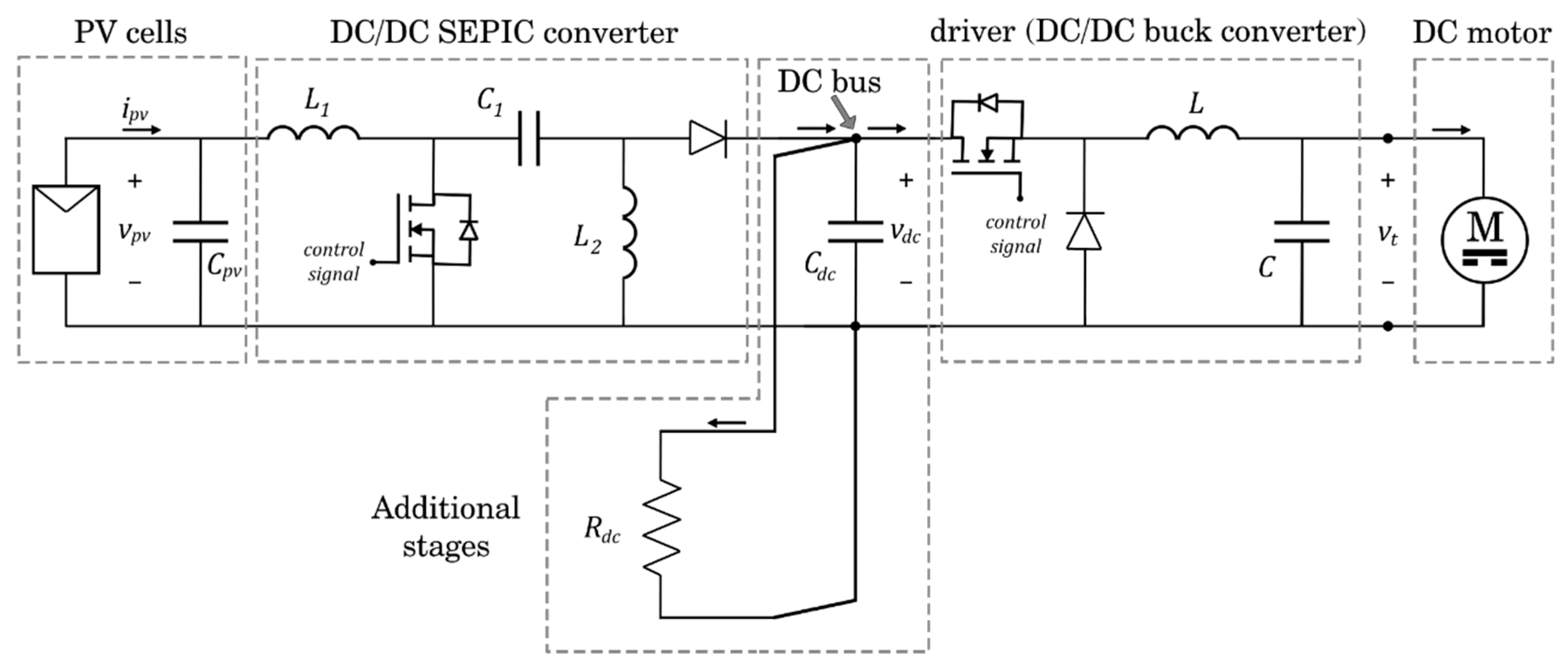
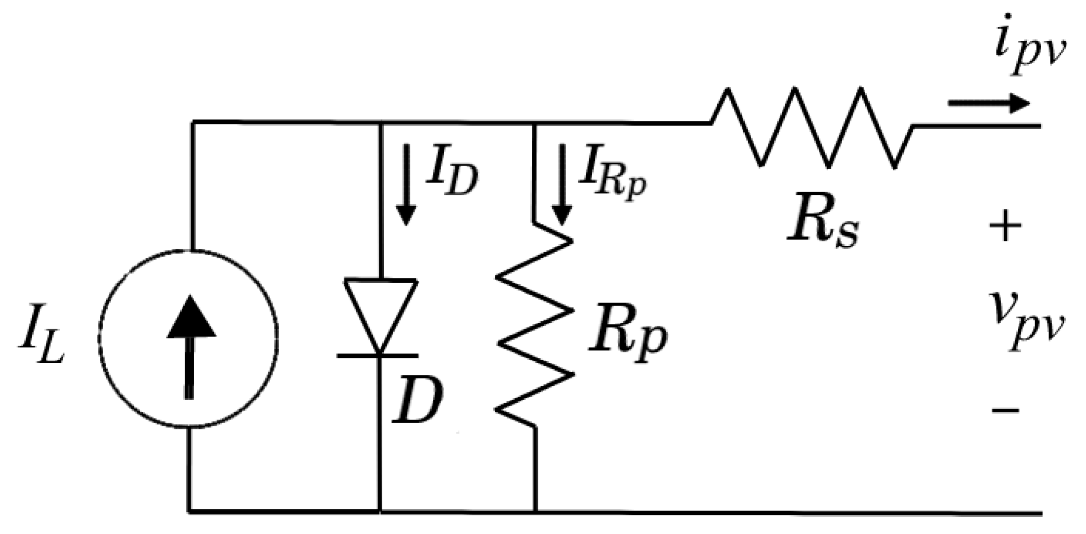
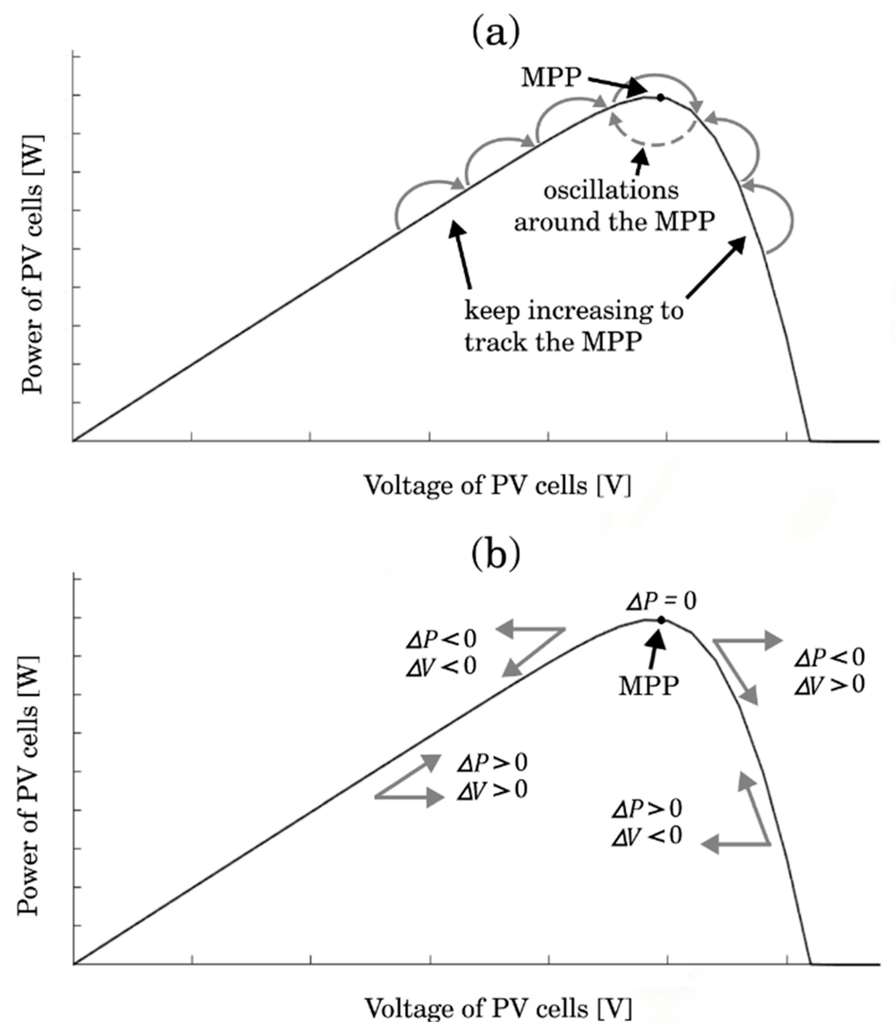
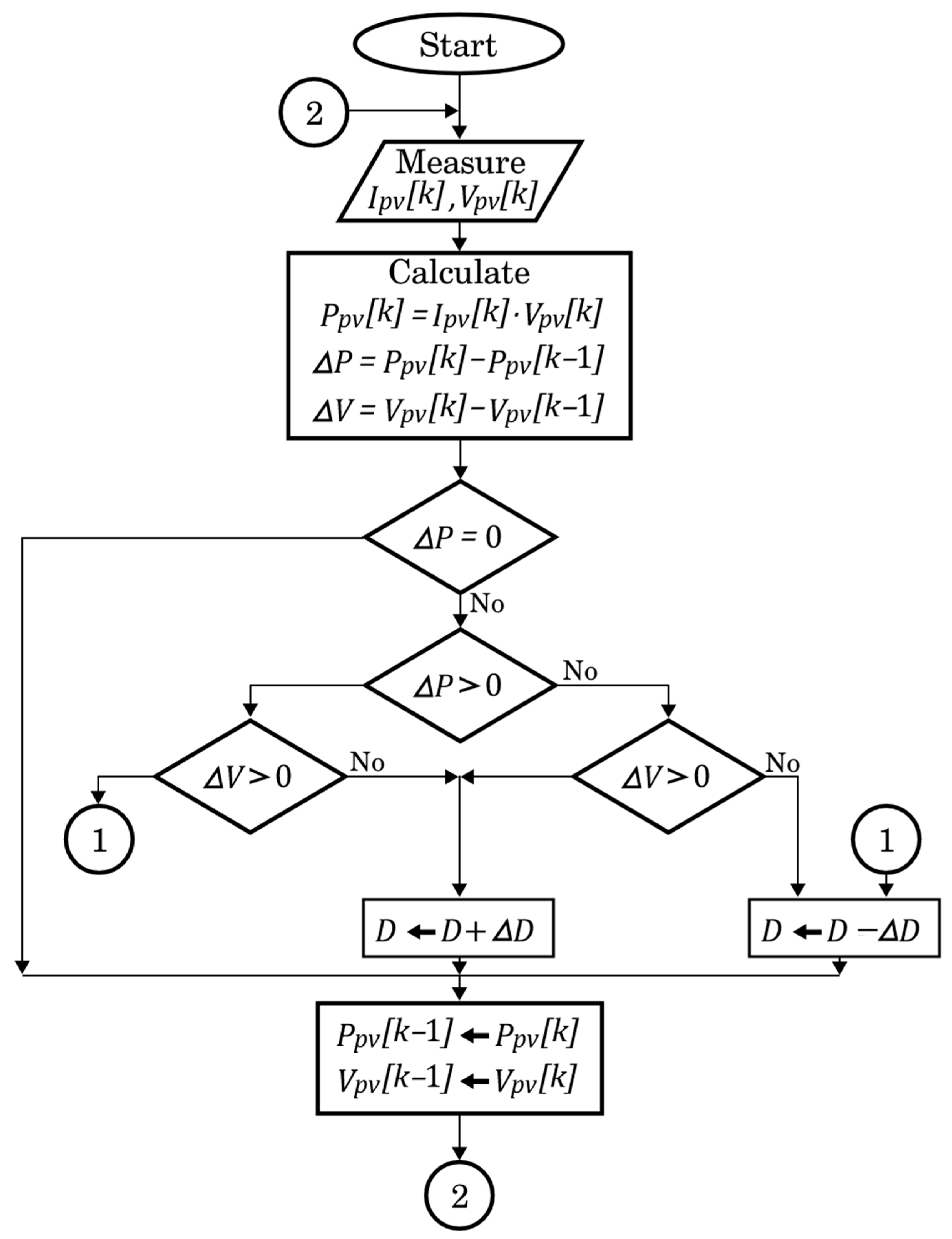
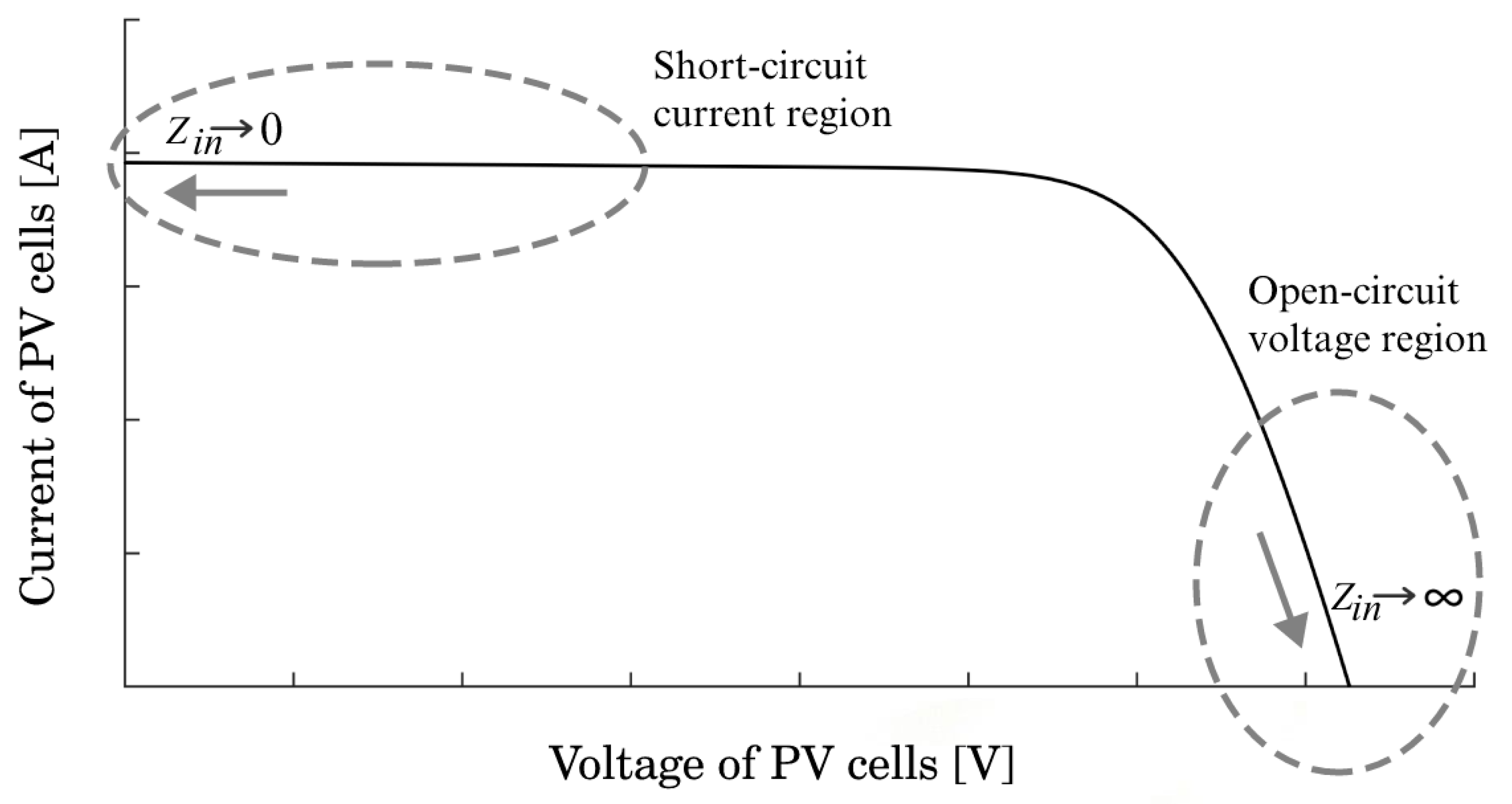
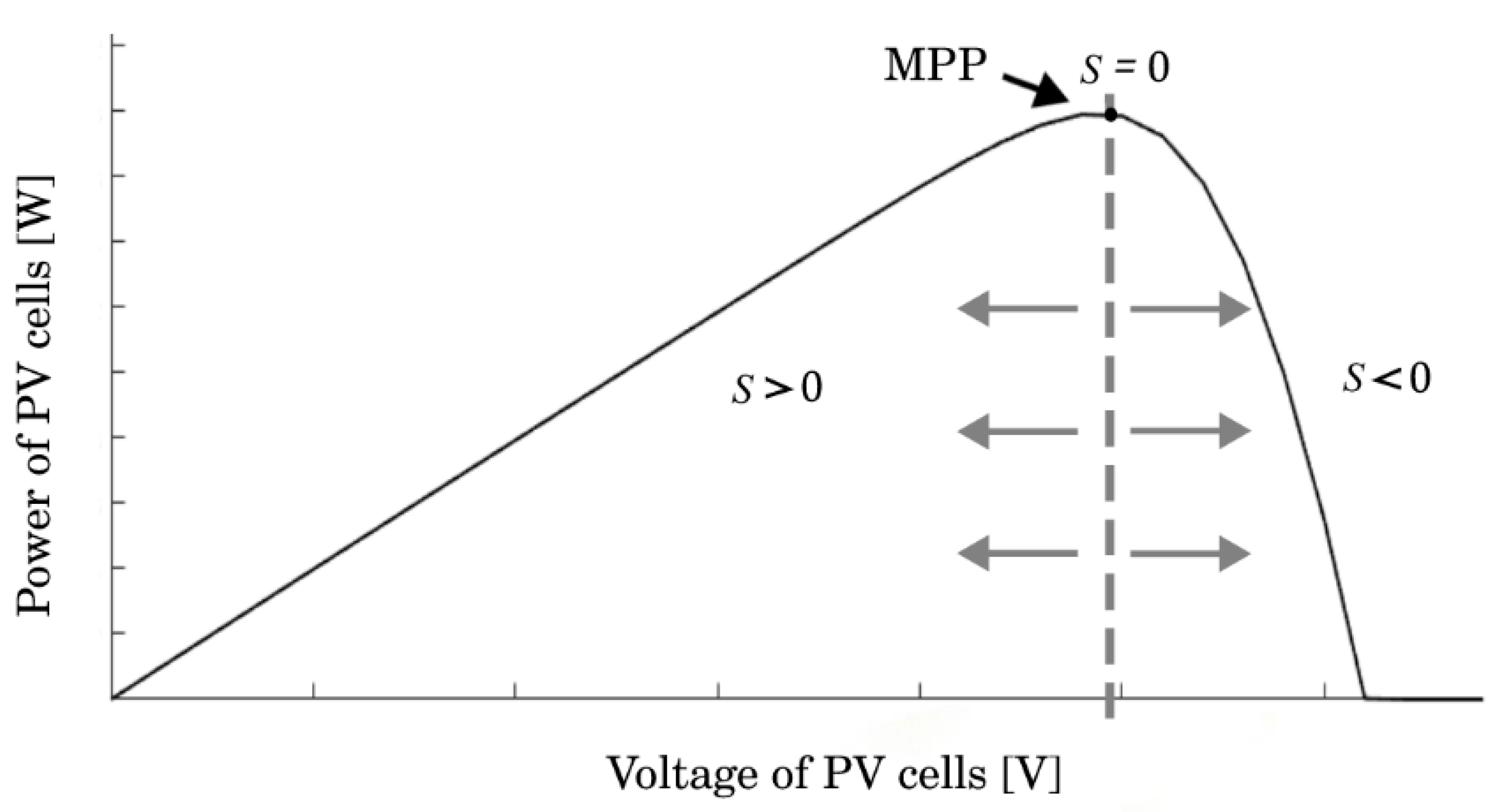

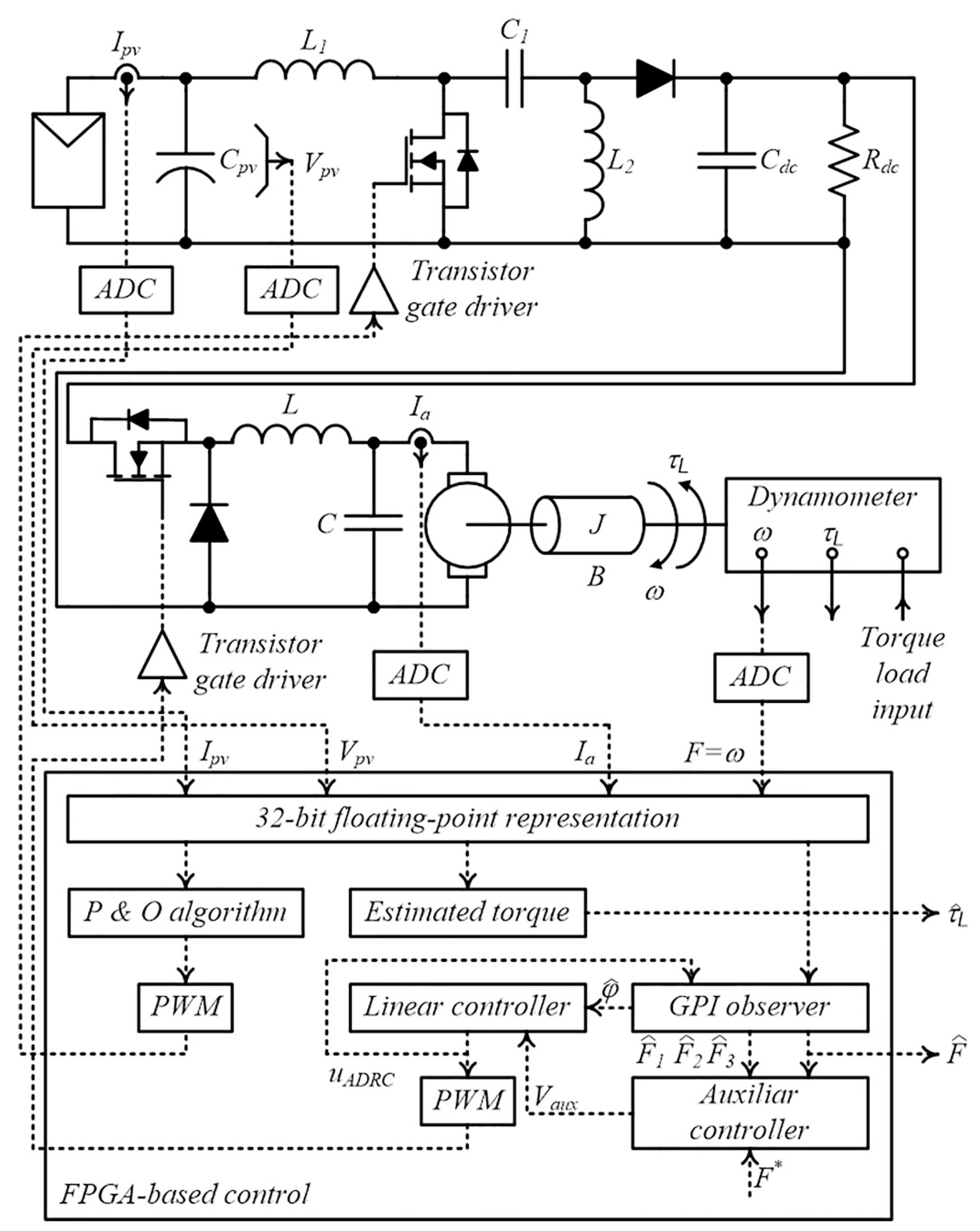
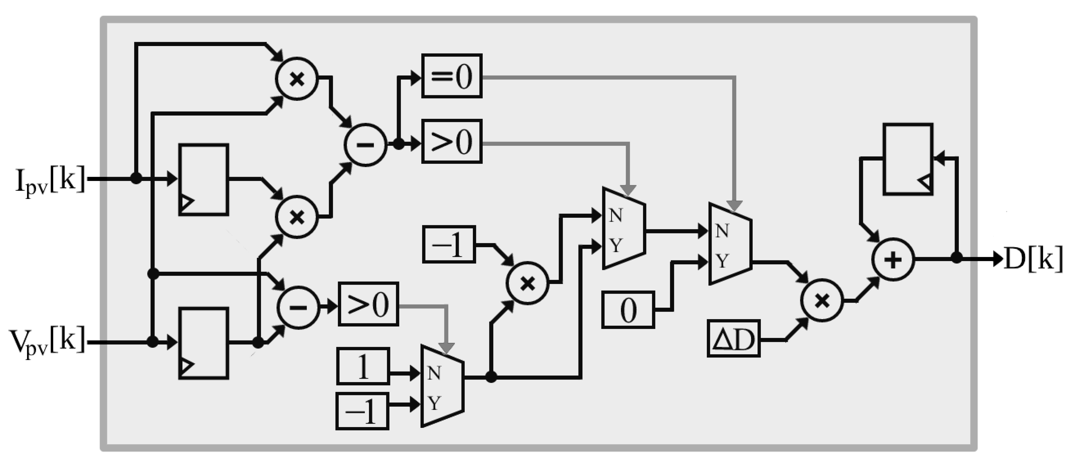
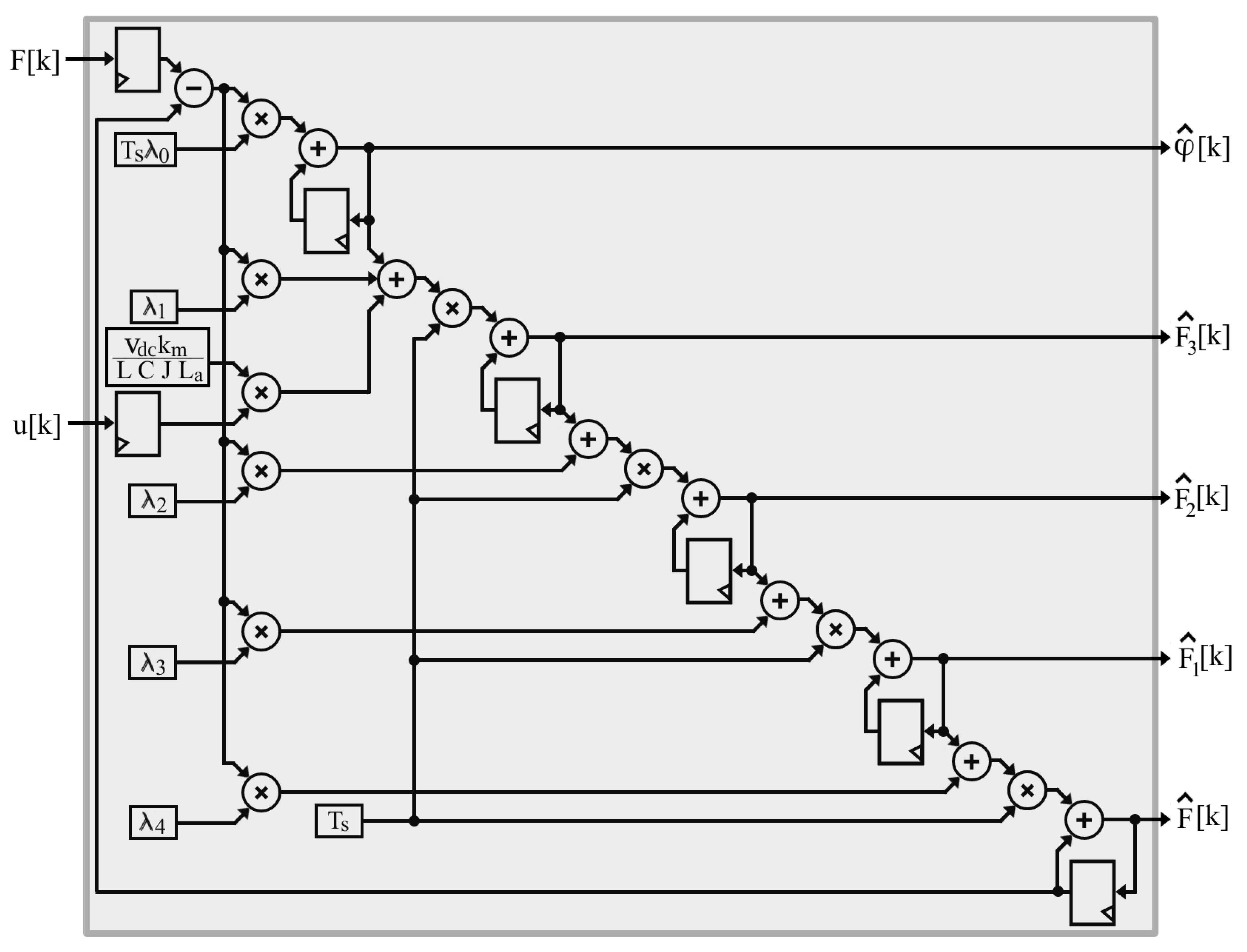
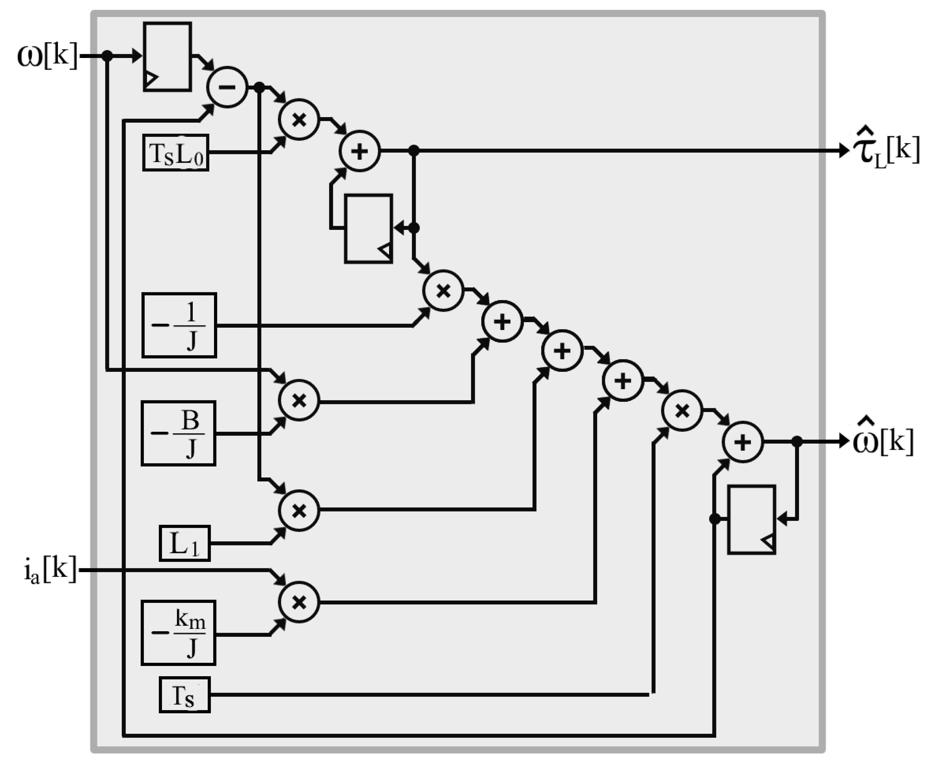


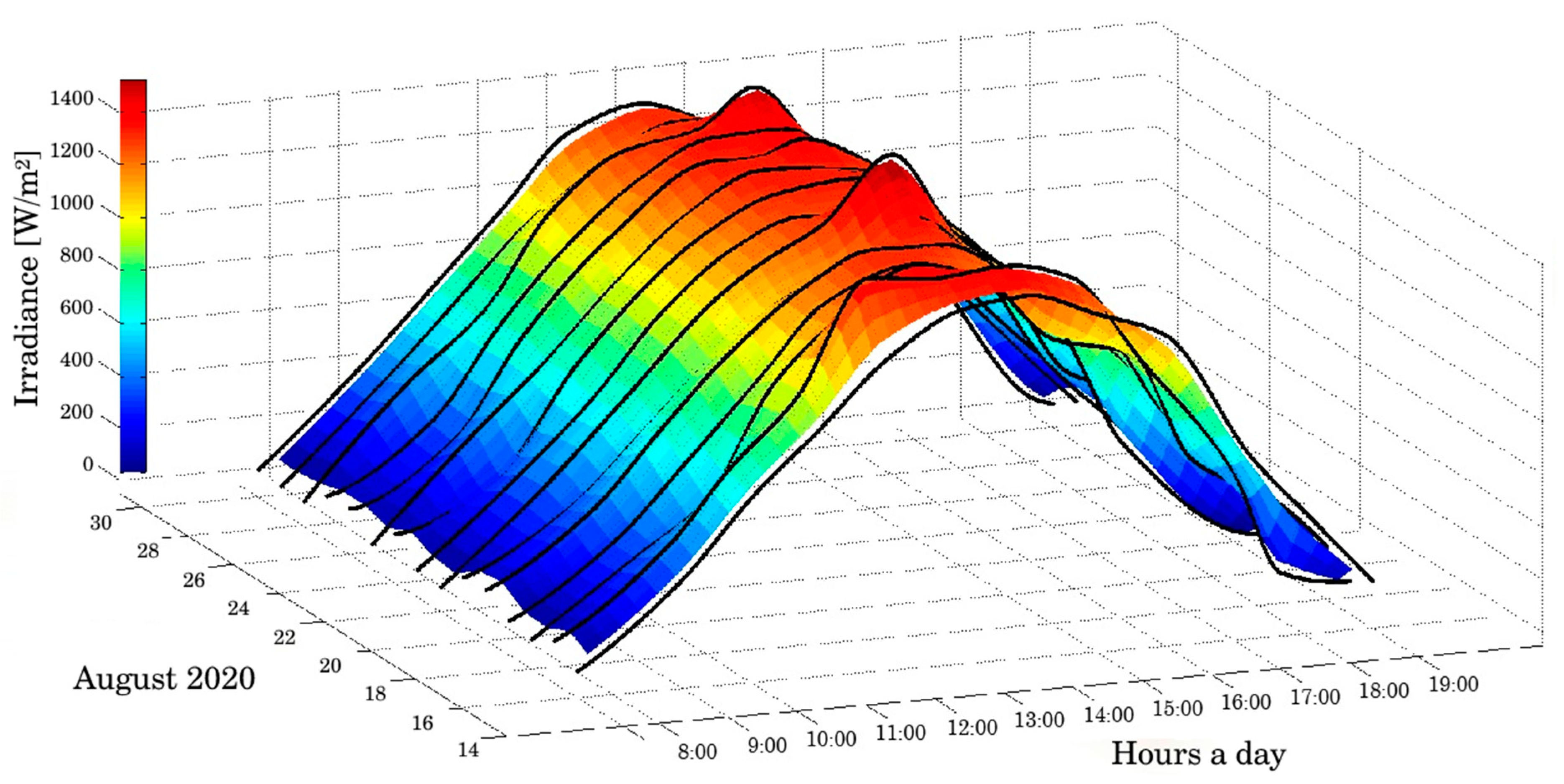

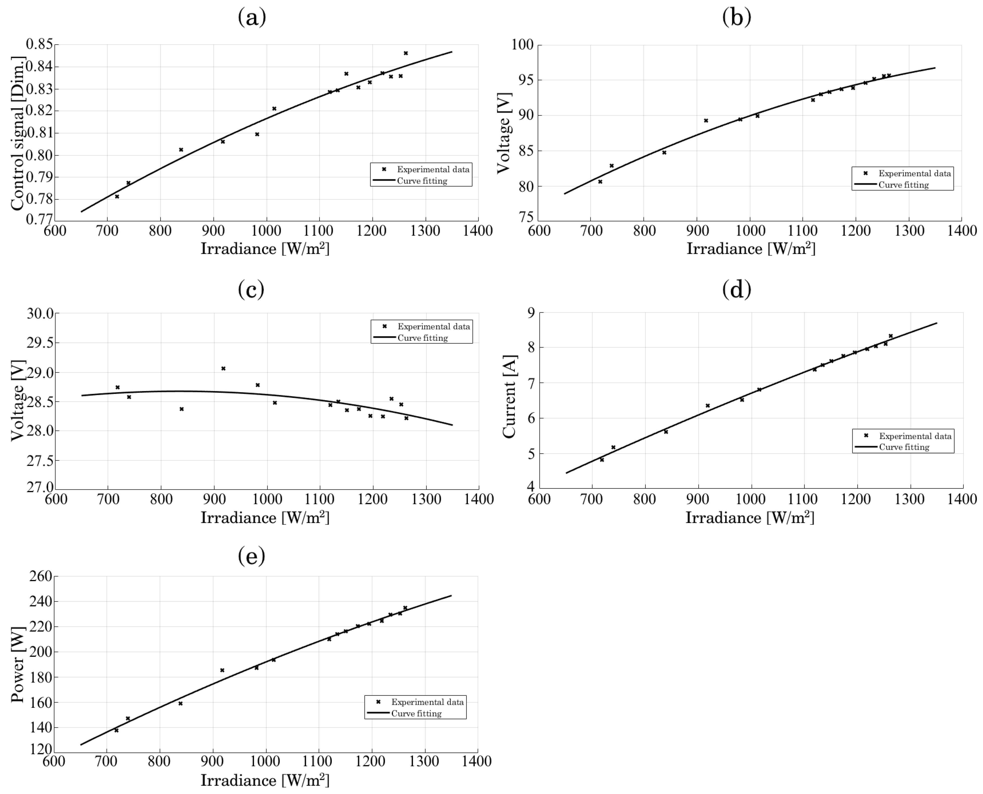
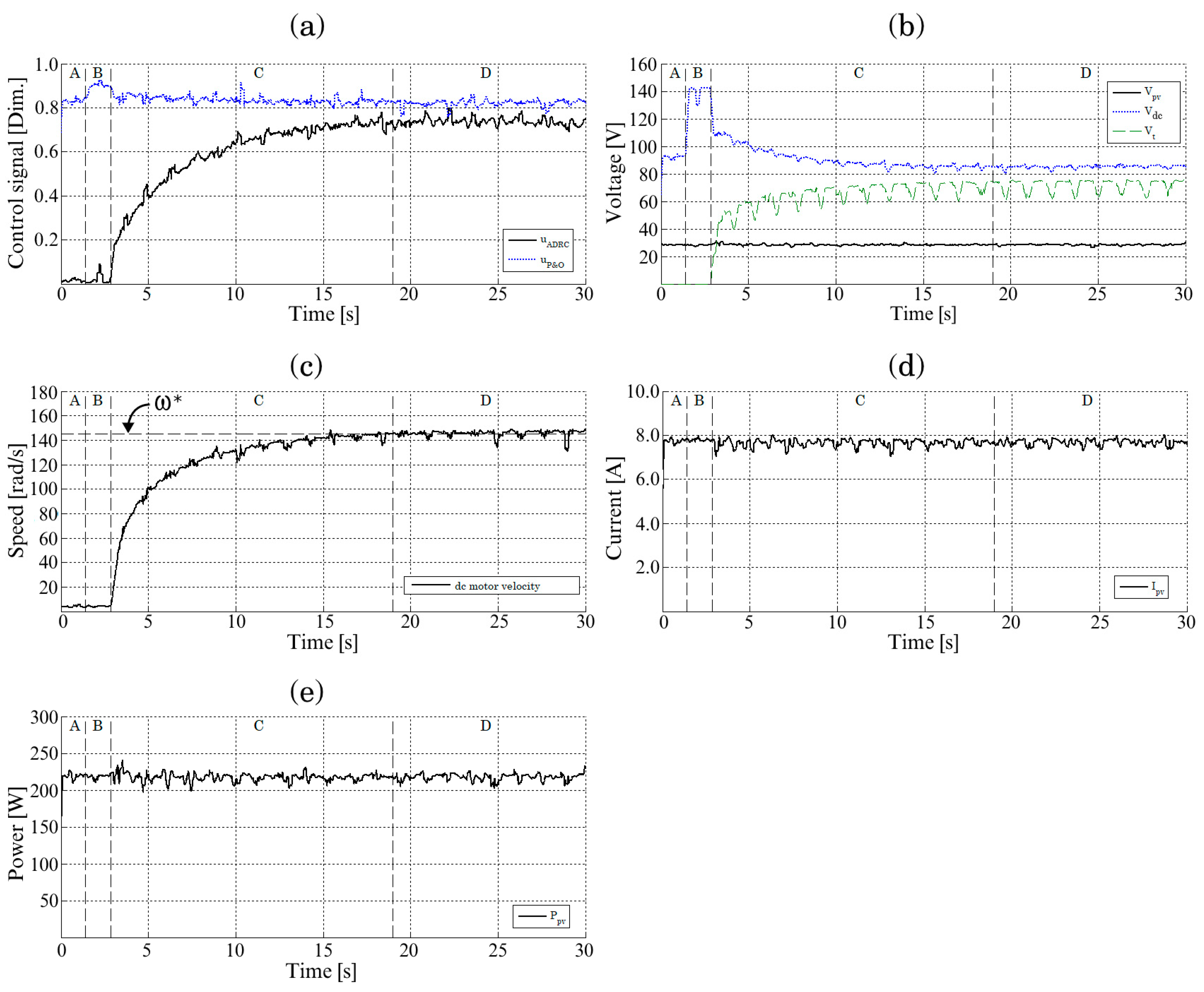


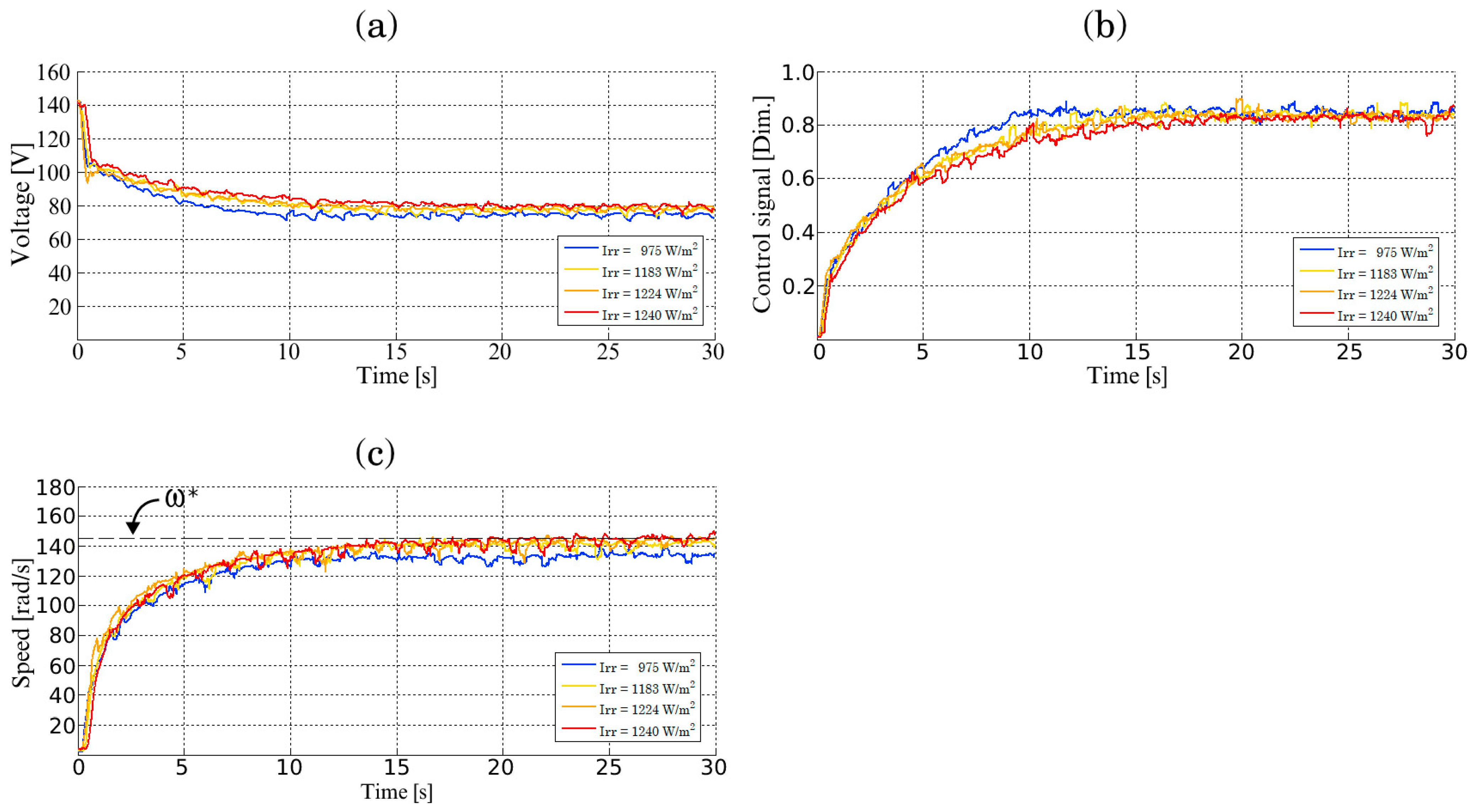
Publisher’s Note: MDPI stays neutral with regard to jurisdictional claims in published maps and institutional affiliations. |
© 2022 by the authors. Licensee MDPI, Basel, Switzerland. This article is an open access article distributed under the terms and conditions of the Creative Commons Attribution (CC BY) license (https://creativecommons.org/licenses/by/4.0/).