Deviation from Darcy Law in Porous Media Due to Reverse Osmosis: Pore-Scale Approach

Abstract

Shale and tight hydrocarbons are vital to global energy dynamics. The fluid flow in sub-micron pores of tight oil reservoirs varies from bulk fluid flow. The Darcy law is widely accepted to model creeping flow in petroleum reservoirs. However, traditional reservoir modeling approaches fail to account for the sub-micron mechanisms that govern fluid flow. The accuracy of tight oil reservoir simulators has been improved by incorporating the influence of sub-micron effects. However, there are still factors that affect sub-micron fluid mobility that need investigation. The influence of a chemical potential gradient on fluid flow in sub-micron pores was modeled by solving Darcy and the transport and diluted species equations. The findings indicate that when a chemical potential gradient acts in the opposite direction of a hydraulic pressure gradient (reverse osmosis), there exists a limiting pressure threshold below which a non-linear flow pattern deviating from the Darcy equation is observed. Furthermore, the simulation based on tight reservoir pore parameters shows that when the effect of a chemical potential gradient is added, the resultant flux is 8–49% less. Hence, including the effect of the chemical potential gradient will improve the accuracy of sub-micron pressure dynamics and flow velocity.

1. Introduction

Understanding the processes that govern fluid flow in porous media has enhanced water purification, fossil fuel recovery, microfluidic product design, and construction [1,2,3,4]. These advances could be credited to the improvement in the system of equations that are used in modeling fluid flow in porous media [5,6]. In recent years, the exploitation of oil and gas resources has shifted to tight reservoirs and shale reservoirs in order to satisfy the rising energy demand since most conventional reserves are nearing the end of their development [7]. However, there are numerous challenges in the exploration of tight and shale oil reserves [8]. One of these challenges is the inability of conventional numerical reservoir simulators to accurately model fluid flow in shales and tight reservoirs due to a low permeability and a high ratio of micron and sub-micron pores compared to conventional reservoirs [9]. The flow in sub-micron pores differs from bulk fluid flow. The sub-micron flow pattern is characterized by boundary layer effects and confinement effects —surface roughness, electric double layer, apparent viscosity, multiphase flow selectivity, and non-linear flow [10,11,12,13,14]. In addition, advances in pore imaging techniques and digital rock physics have shown that the micron and sub-micron pores contribute significantly to the filtration process in tight and shale reservoirs [15,16]. Hence, the contribution of micron and sub-micron pores to the hydrocarbon reservoir drainage cannot be overlooked. To achieve accurate simulation results in the modeling of fluid filtration in shale and tight oil deposits, numerical reservoir simulators must account for all pertinent sub-micron processes and flow behavior.

Conventionally, the flow in porous media is described by the Darcy law, which is expressed mathematically as: $v_x=\left(k/\mu \right)\left(\nabla p\right)$ [17]. Where $v_x$ is the fluid flux per unit of the medium with viscosity $\left(\mu \right)$, the permeability of the porous medium $\left(k\right)$, and a pressure gradient $\left(\nabla p\right)$ across the medium. Even though the Darcy law is generally accepted and has been validated by numerous experiments, other studies have shown how fluid flow in porous media could deviate from the Darcy law [18,19,20,21,22,23,24,25,26,27].

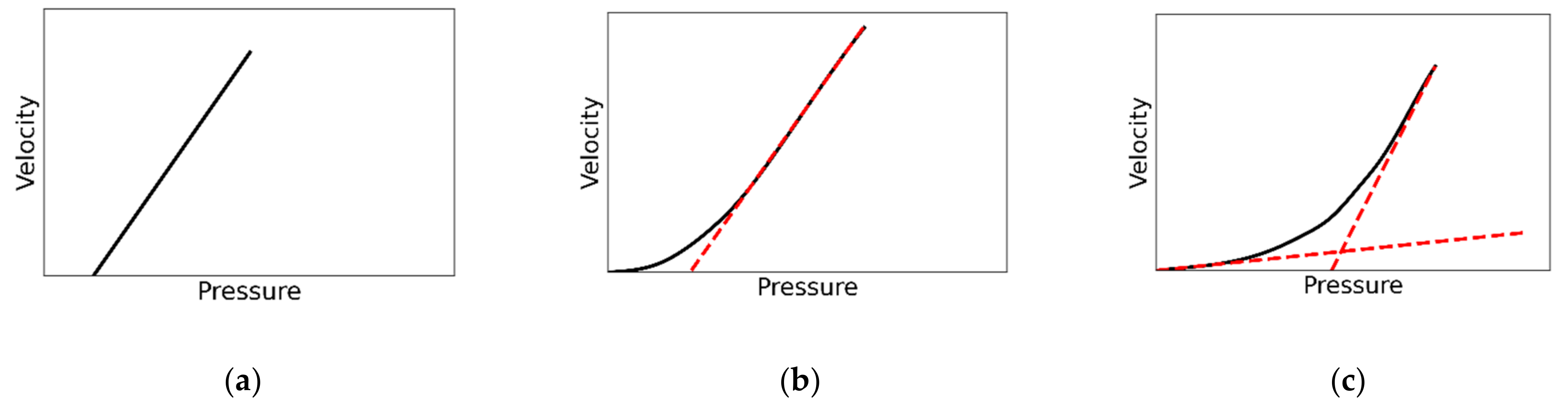
Dudgeon [21] conducted a series of tests on consolidated core samples and presented results that indicated the presence of three regimes of fluid flow in porous media. Later, Basak [28] confirmed the results of Dudgeon [21] and classified these regimes as Pre-Darcian, Darcian, and Post-Darcian. Other research similar to the work of Dudgeon and Basak was conducted but was mainly focused on water/brine filtration for water treatment systems [29]. An experimental test by Siddiqui et al. [27] and Kececioglu and Jiang [30] on consolidated cores showed that the departure from the Darcy law could result in the underprediction of reserves and prospecting opportunities for petroleum resources. The reported mechanisms and flow conditions that result in a non-Darcian flow include low pressure gas limitations [31], non-Newtonian fluid [32], a high velocity stable flow [33], interstitial pore space curvature [34], a viscous boundary layer [35], osmosis [19,36,37], flow in non-straight channels [38], and flow in rough-walled channels [39,40]. Kutilek [41] made a summary of the experiments that did not follow the Darcy law (Figure 1).

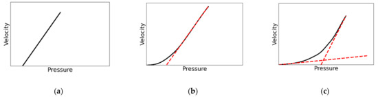
Figure 1. Pre-Darcian, Darcian, and Post Darcian curves—pressure and velocity relationship as grouped by Kutilek [41]. Black continuous line shows the non-linearity of Darcy law. Red-dashed line shows the expected linearity of Darcy law. (a) Linear proportionality between pressure and velocity with the curve not passing through the origin. (b) A non-linear proportionality between pressure and velocity at lower pressure and a linear proportionality at relatively higher pressure. (c) Non-linear proportionality between pressure and velocity.

An experiment conducted by Churaev [19] on the filtration of a dilute solution through a membrane showed that the curve of the hydraulic pressure against the measured flux did not agree with the Darcy law at a lower pressure difference. However, linearity between the pressure and the flux is observed at a relatively higher pressure difference. The curve obtained by Churaev [19] has two segments: a Pre-Darcian segment at a lower pressure drop and a Darcian segment at a higher pressure drop. These curves are similar to the curves from Kutilek [41]’s classification, as shown in Figure 1a–c. Churaev [19] concluded that the occurrence of non-linearity of the Darcy law is due to a solute concentration gradient developed across the membrane in a process referred to as reverse osmosis [42,43,44,45]. Moreover, other studies have indicated and suggested that certain subsurface lithology types such as clays, shales, siltstones, and zeolites at the micron and sub-micron scale possess selectivity characteristics: a semi-permeable membrane [46]. The selectivity characteristic leads to the development of a chemical potential gradient in the micron and sub-micron pores.

This current research investigated the formation of a chemical potential gradient in a reverse direction to the hydraulic pressure gradient at the pore scale. Limiting pressure beyond which there is linearity between the flux and the pressure and below which there is non-linearity presented by computing the Darcy equation coupled with the diffusion-convection equation. Incorporating the influence of a chemical potential gradient into shale and tight oil simulators will improve the accuracy of estimating the precise proportionality between the flux (flow velocity) and the pressure gradient at the micron and sub-micron scales. This study is divided into three main parts: Section 2 presents the theoretical background of reverse osmosis and the description of the numerical model. The simulation results are presented and discussed in Section 3 and summarized in the conclusions (Section 4).

2. Numerical Analysis

2.1. Theory

The solvent flux is the volumetric flow rate of the solvent across a unit area of the membrane. In the absence of hydraulic pressure (where only the osmotic pressure is the driving force), the solvent flux across the semi-permeable membrane is given by Equation (1) [47,48].

$$J_w=A·\Delta \pi$$

(1)

where $J_w$ is the solvent flux and $A$ is the pure solvent permeability over the medium across which the osmotic pressure drop is acting. From the Darcy law, $A$ is given by $\left(k/\mu L\right)$, where $k$ is the permeability of the porous medium, $\mu$ is the viscosity of the fluid, and $L$ is the length of the flow path. The osmotic pressure is given as $\pi =rRTc,$ and the osmotic pressure difference across the membrane is given by $\Delta \pi ={\pi }_f-{\pi }_p$. Here, $r$ is the retention coefficient, $R$ is the ideal gas constant $\left({\mathrm{JK}}^{-1}{\mathrm{mol}}^{-1}\right)$, $T$ is the absolute temperature $\left(K\right)$, $c$ is the molar concentration $\left(\mathrm{mol}/{\mathrm{m}}^3\right)$, and subscripts $f$ and $p$ are membrane interface at the feed-side and the permeate side, respectively (Figure 2). The resultant solvent flux $\left(J_w\right)$ in the presence of applied hydraulic pressure difference $\left(\Delta p=p_1-p_2\right)$ and the osmotic pressure difference $\left(\Delta \pi \right)$ becomes Equation (2). The value of the pure solvent permeability ($A$) in Equation (2) changes with respect to the permeability $\left(k\right)$ and the length of the domain $\left(L\right)$ across which the respective pressures are acting.

$$J_w=A\Delta p-A\Delta \pi$$

(2)

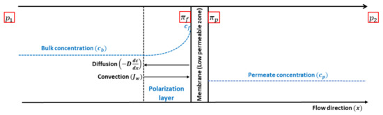
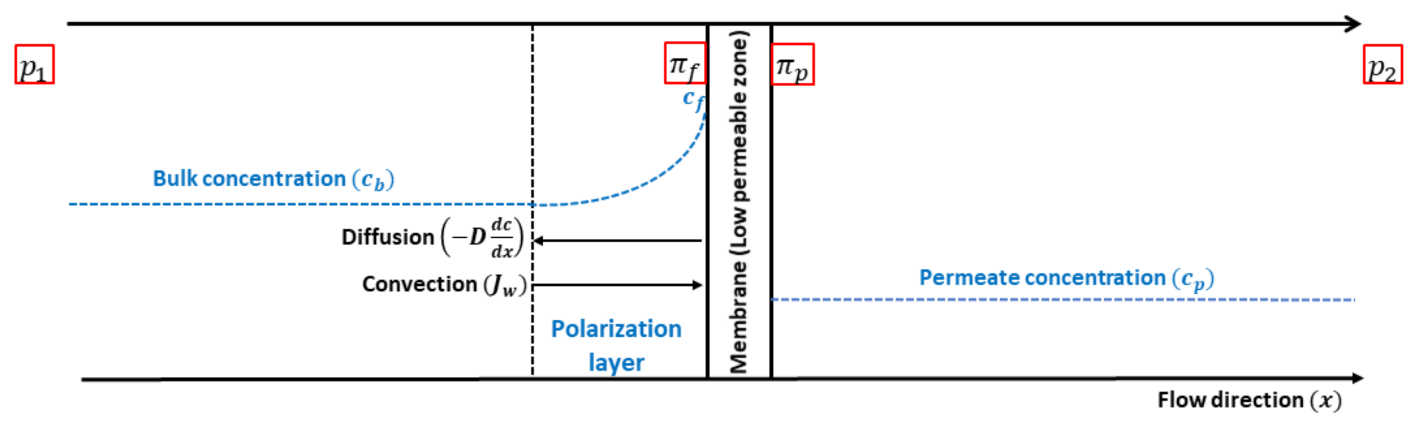
Figure 2. Graphical representation of concentration polarization due to reverse osmosis. $J_w$ represents the resultant solvent flux, $c$ represents the concentration, $\pi$ represents the osmotic pressure, and $p$ represents the applied hydraulic pressure. The subscript $b,f,p$ represent the bulk concentration, the solute concentration on the wall of the membrane at the feed-side and the permeate solution, respectively. Subscripts 1 and 2 represent the inlet and outlet of the channel, respectively.

2.2. Computational Domain

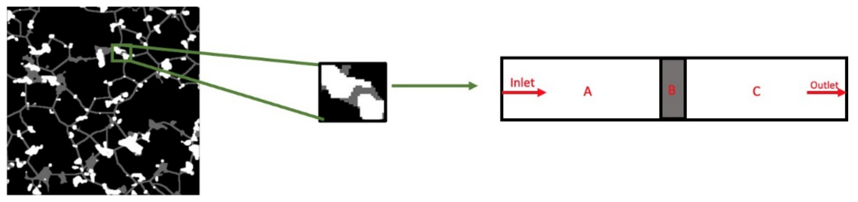
A channel with regular geometry was simulated under steady-state and standard conditions. The range of geological properties for the simulation was chosen to cover the micron and sub-micron pore spectrum. For simplification, the model was developed to represent a low permeability zone between two relatively higher permeability zones, as presented in Figure 3.

Figure 3. Schematic representation of the simulated geometry.

The grey zones (Zone B) represent the low permeability zone, and the white zones (Zone A and C) represent the relatively high permeability zones. The low permeable zone is assumed to have the characteristics of a semi-permeable membrane as reported by [46,49,50,51,52]. The dimension of the simulated model is 105 µm × 5 µm. Zones A and C of the model have a length of 50 µm each, while Zone B has a length of 5 µm.

2.3. Governing Equations and Boundary Conditions

The driving force of fluid flow in the presented model is controlled by the pressure drop along the channel and the osmotic pressure across the membrane. To solve this physical problem of flow in porous media and the transport of diluted species, the general form of porous media fluid flow (Equation (3)) was coupled with the convection-diffusion equation (Equation (4)).

$$\frac{\partial }{\partial t}\left(\rho {\epsilon }_p\right)+\nabla ·\left(\rho u\right)=Q_m$$

(3)

$$\frac{\partial c}{\partial t}=\nabla ·\left(D\nabla c\right)-\nabla ·\left(uc\right)+R$$

(4)

where $\rho$ is the fluid density $\left(\mathrm{kg}/{\mathrm{m}}^3\right)$, ${\epsilon }_p$ is the model porosity, $u=\left(u,v,w\right)$ is the hypothetical superficial velocity vector $\left(\mathrm{m}/\mathrm{s}\right)$, $Q_m$ is the mass source $\left(\mathrm{mol}/{\mathrm{m}}^2·\mathrm{s}\right)$, $c$ is the solute concentration $\left(\mathrm{mol}/{\mathrm{m}}^3\right)$, $D$ is the diffusion coefficient, and $R$ is a source term for reaction rate expression for the species $\left(\mathrm{mol}/{\mathrm{m}}^3·\mathrm{s}\right)$. Considering the presented model at a steady and isothermal state with an incompressible fluid, non-inertial flow, constant porosity, constant fluid density, and no source term of mass and reaction rate, Equation (3) reduces to Equation (5). Similarly, Equation (4), under similar assumptions, reduces to Equation (6). Each region of the geometry is assumed to be isotropic; hence the permeability value is taken as a scalar [53].

$$\nabla ·u=0$$

(5)

$$0=\nabla ·\left(D\nabla c\right)-\nabla ·\left(uc\right)$$

(6)

When a fraction of the solute molecules is retained on the feed side of the semi-permeable membrane, the solute concentration will continue to build upon the membrane walls at the feed side. This phenomenon is termed “concentration polarization” (Figure 2) [54]. Due to concentration polarization, a boundary layer known as the polarized layer is formed. Different methods such as the classic solution-diffusion model, film theory model, and the electrolyte theory model are normally used to compute the polarized layer concentration, the concentration on the wall of the membrane at the feed-side and the permeate concentration [48]. At a steady state, the convection and diffusion process in the polarized layer reach equilibrium—the film theory assumes a multi-dimensional transport problem as a one-dimensional transport problem, as given in Equation (7). From the film theory, the relationship between the bulk concentration $\left(c_b\right)$, the concentration on the interface of the membrane $\left(c_f, c_p\right)$, and the resultant flux $\left(J_w\right)$ can be obtained by integrating the one-dimensional diffusion equation from the membrane interface (between zone A and B), out along the thickness of the polarized layer $\left(\delta \right)$, which can be presented as Equation (8) [47,48,55,56]. The film theory model describes the solute accumulation at the membrane walls where the solute is transferred by convection towards the membrane and by diffusion in the opposite direction into the bulk solution [57,58,59].

$$J_{w}c+D\frac{\partial c}{\partial x}=0$$

(7)

$$\frac{c_f-c_p}{c_b-c_p}=\exp \left(\frac{J_w}{K}\right)$$

(8)

$c_b$ is the bulk concentration, $c_p$ is the concentration on the membrane interface between zone B and C, $c_f$ is the concentration on the membrane interface between zone A and B, $J_w$ is the resultant solvent flux, and $K$ is the mass transfer coefficient $\left(K=Sh\left(D/d_h\right)=\left(D/\delta \right)\right)$, where $Sh$ is the Sherwood number, $D$ is the solute diffusivity coefficient, and $d_h$ is the characteristic length (diameter of the channel). The Sherwood number ($Sh$) under laminar flow is given by $Sh={\left(Re·Sc·\frac{d_h}{L}\right)}^{\left(1/3\right)}$ [60]. Where $Re$ is the Reynolds number, $Sc$ is the Schmidt number, $d_h$ is the diameter of the channel, and $L$ is the length of the flow path. The Reynolds number ($Re$) is given by ($Re=\left(\rho u{d}_h\right)/\mu$) and the Schmidt number ($Sc)$ is given by ($Sc=\mu /\left(\rho D\right)$), where $\rho$ is the density of the fluid, and $\mu$ is the viscosity of the fluid.

Due to the solute retention on one side of the membrane, the mass balance between the solute concentration on either side of the membrane can be accounted for by introducing the retention coefficient into Equation (7) [60]. The solute concentration on the interface of the membrane between zone A and zone B and between zone B and zone C is given by Equations (9) and (10) to account for mass balance on both sides of the interface of the membrane, respectively. A drawback of this approach is that the film theory does not account for solute transport within the membrane [61].

$$D\frac{\partial c}{\partial x}+J_{w }{c}_{f}r=0$$

(9)

$$D\frac{\partial c}{\partial x}+J_w{c}_p=J_{w }\left(1-r\right)c_f$$

(10)

The retention coefficient $\left(r\right)$ can be determined as presented in Equation (11) [62]. The retention coefficient is the ratio of the concentration of solute molecules in the permeate solution to the solute concentration in the bulk solution [63]. The value of $r$ is between zero and one $(0<r<1)$ [62]. Once the retention coefficient is known, the value of the permeate concentration on the wall of the membrane $c_p$ can be determined by Equation (12).

$$r=1-\frac{1}{S}\left[\frac{\left({\overline{V}}_s{c}_b+\lambda \right)\Delta p-\lambda nRT{c}_{b}r-nRT{c}_{b}ln\left(1-r\right)}{\Delta p-nRT{c}_{b}r}\right]$$

(11)

$$c_p=\left(1-r\right)·c_b$$

(12)

where, $c_b$ is the bulk concentration, ${\overline{V}}_s$, is the partial molar volume of solute, $S$ is the selectivity coefficient of the membrane, $n$ is the number of ions ionized from a salt molecule, $\lambda$ is the ratio of solute radius to pore radius, and $\Delta p$ is the applied hydraulic pressure difference. Since Equation (11) is defined implicitly, an iterative method was used to determine the value of $r$ with the lowest possible margin of error. The selectivity coefficient was approximated as $\left(S=1/\left(1-r_{\max }\right)\right)$ where $r_{\max }$ is the maximum retention [19]. At $r_{\max }$, the value of $r$ does not change with respect to the increasing pressure. The maximum retention coefficient was computed by Equation (13), where $\lambda$ is the ratio of the radius of solute molecules $\left(r_s\right)$ to the pore radius of the membrane $\left(r_p\right)$.

$$r_{\max }=1-\left(1-{\left(\lambda \left(2-\lambda \right)\right)}^2\right)·\exp \left(-0.7146{\lambda }^2\right)$$

(13)

The resultant flux $\left(J_w\right)$ under the influence of applied hydraulic pressure and a chemical potential gradient, that acts in the opposite direction, is given by Equation (2), where $\Delta p$ is the applied hydraulic pressure drop across the entire channel and $\Delta \pi$ is the pressure drop due to the chemical potential gradient across the membrane. Equation (2) shows that the resultant flux $\left(J_w\right)$ is the sum of the flux due to the applied hydraulic pressure drop $\left(\Delta p\right)$ and the flux due to the chemical potential gradient (which act in opposing directions in this study).

The hydraulic pressure drop over the domain was computed by imposing an inlet boundary condition axial velocity $\left(u=u_0\right)$ while the transverse velocity $\left(v=0\right)$ was assumed as zero (Table 1). At the outlet of the model, a pressure $\left(p_2\right)$ was specified, where the pressure $p_1$ imposed by $u_0$ is higher than $p_2$ ($p_1$ > $p_2$). A no flux and no-slip boundary condition were specified on the impermeable walls of the channel. At this initial stage, no chemical potential gradient was considered in the model. This gave the applied hydraulic pressure drop ($\Delta p=p_1-p_2$) over the entire domain. From Equation (2), the value of the pure water permeability $\left(A\right)$, for the $\left(\Delta p\right)$ and the chemical potential gradient $\left(\Delta \pi \right)$ are not equal. Hence, effective permeability for the computation of the flux due to $\Delta p$ was computed by the harmonic averaging method $\left(k_{avg}=L/\left(L_A/k_A+L_B/k_B+L_C/k_C\right)\right)$. Where $L$ is the total length of the channel $\left(L_A+L_B+L_C\right)$ and $k_A$, $k_B$, and $k_C$ are values of permeability of the different zones [64].

Table 1. Summary of boundary conditions.

Boundary	Condition	Parameter
Inlet	Velocity	$u=u_0;v=0$
Inlet	Bulk concentration	$c=c_b$
Outlet	Pressure	$p=p_2$
Channel wall	No-flow, No-slip	$u,v=0, c=0$

To compute the pressure drop across the membrane due to chemical potential gradient $\left(\Delta \pi \right)$, Equation (2) can be rewritten as Equation (14) by substituting in the variables of the chemical potential gradient. There are two unknown variables $\left(c_f \mathrm{and} J_w\right)$ in Equation (14). Hence, Equations (9) and (14) are solved simultaneously by an iterative process to determine concentration on the membrane interface $\left(c_f\right)$ and the resultant flux of the fluid $\left(J_w\right)$ under the influence of both the applied hydraulic pressure and the chemical potential gradient.

$$J_w=\left(A\Delta p\right)-\left(rART\left(c_f-c_p\right)\right)$$

(14)

3. Results and Discussion

3.1. Model Validation

To understand the model’s performance and stability, the results were compared with experimental results presented by Churaev [19]. The result from Churaev [19] was conducted with a KCl solution. The bulk concentration ($c_b$) of the solution is 1000 $\mathrm{mol}/{\mathrm{m}}^3.$ Since the value of the permeability coefficient ($A$) was not directly stated in the experiment by Churaev [19] it was calculated from the linear section of the curve of resultant flux against the pressure gradient, as presented in Figure 4a. The calculated value of the pure solvent permeability coefficient ($A$) is $2.96 · {10}^{-12} \left(\mathrm{m}/\mathrm{Pa}.\mathrm{s}\right)$ and the value of the selectivity coefficient $\left(S\right)$ of the membrane used in the experiment is 25. In addition, the density and viscosity were assumed to be water, as presented in Table 2. To compare the curves of resultant flux against pressure drop, the percentage deviation was computed by Equation (15) for the simulated pressure range.

$$Percentage deviation=\frac{original value-obtained value}{original value} ·100\%$$

(15)

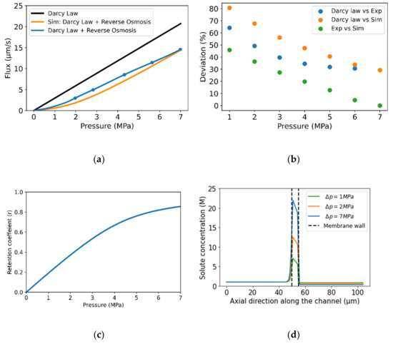
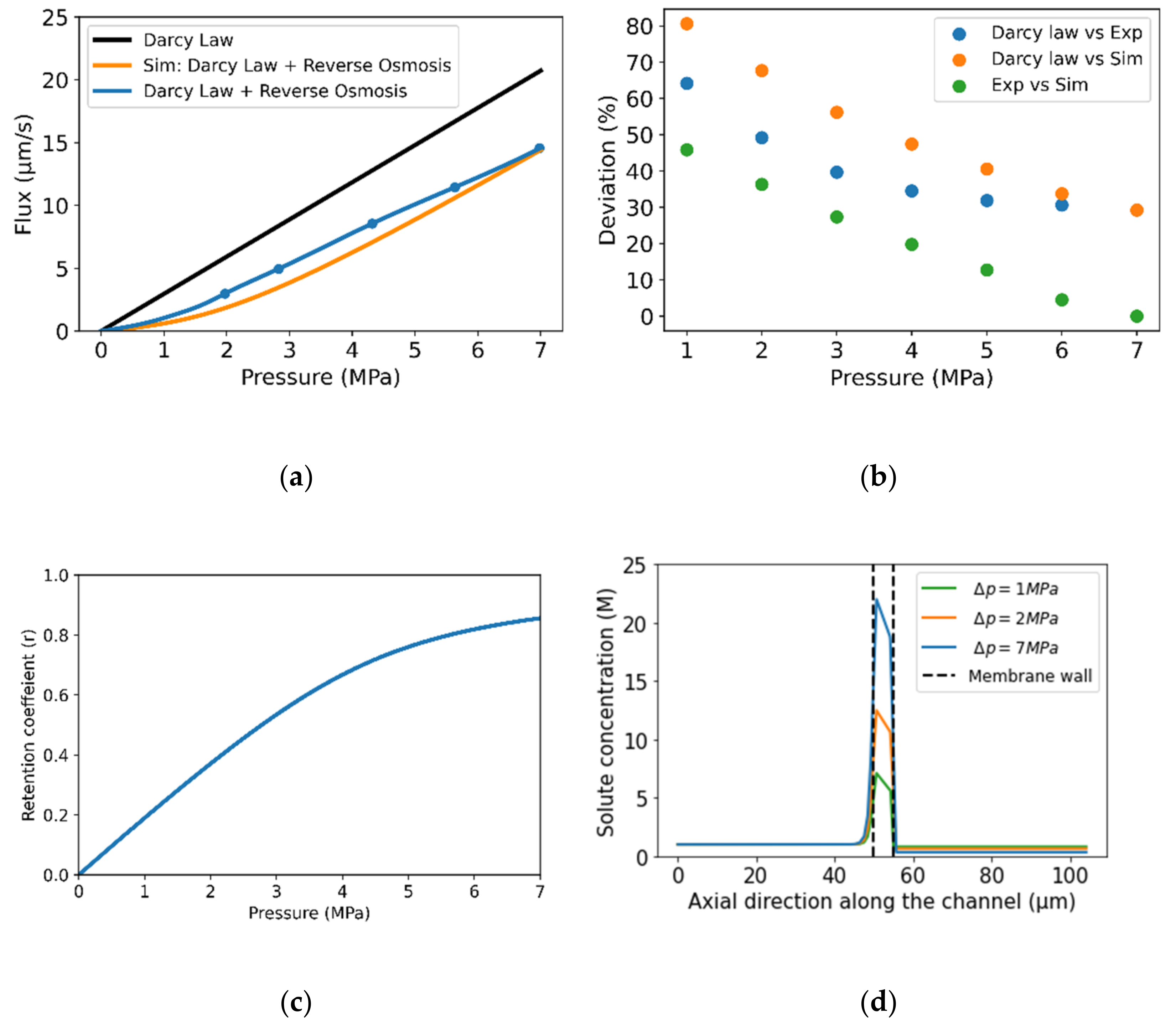
Figure 4. (a) Comparison of Darcy law (without the effect of reverse osmosis) and the experimental and numerical results (with the effect of reverse osmosis). (b) Percentage deviation of experimental and simulated results from the Darcy law. (c) Simulated retention coefficient (r) at different pressure differences. (d) Distribution of solute in the simulated geometry $\left(1\mathrm{M}=1000 \mathrm{mol}/{\mathrm{m}}^3\right)$.

Table 2. Parameters of the numerical model.

Parameter	Unit	Zone A	Zone B	Zone C
Permeability	${\mathrm{m}}^2$	$1.97\times {10}^{-16}$	$9.87\times {10}^{-19}$	$1.97\times {10}^{-16}$
Width	$\mathsf{\mu }\mathrm{m}$	5	5	5
Length	$\mathsf{\mu }\mathrm{m}$	50	5	50
Fluid viscosity	$\mathrm{Pa}·\mathrm{s}$	0.001	0.001	0.001
Fluid density	$\mathrm{kg}/{\mathrm{m}}^3$	1000	1000	1000

The results (Figure 4a) show that the deviation between the experimental (Darcy law + reverse osmosis) and numerical results (Sim: Darcy law + reverse osmosis) varies with pressure. Hence, the results were compared by calculating the percentage deviation for every simulated pressure difference (Figure 4b). The percentage deviation for the experiment and simulation is between 0% and 45%. The highest deviation is associated with the non-linear sections of the curve of resultant flux against the pressure difference (1 MPa and 4 MPa) and decreases as the pressure difference increases. The margin of error of the numerical simulation and the experimental results could result from the approximation of the permeability coefficient $\left(A\right)$, the assumed density and viscosity of the fluid, and the possible errors from the experiment. At the highest simulated pressure point (7 MPa), the numerical results agree with the experiment results.

The comparison shows that both the experiment by Churaev [19] and the numerical simulation presented in this study deviate from the Darcy law when the chemical potential gradient is active in the model (Figure 4a). The percentage deviation for all the simulated pressure ranges is between 30% and 80%. Figure 4c shows that the rate of increase in the retention coefficient decreases with the increasing pressure difference $\left(\Delta p\right)$ across the model, as demonstrated by Song [62]. The distribution of solute concentration in the porous medium at different applied hydraulic pressure(s) is presented in Figure 4d. The solute concentration within the membrane is not accounted for by the methodology used [61]. The thickness of the polarization layer $\left(\delta \right)$ is approximately 4.5µm. The average solute concentration within the polarized layers is 2183 mol/m³, 3273 mol/m³, and 5143 mol/m³ for 1 MPa, 2 MPa, and 7 MPa (applied pressure), respectively.

3.2. Effect of Pore Radius and Bulk Concentration

The model with and without the effect of reverse osmosis was computed. A range of hydraulic pressure difference ($\Delta p$ = 0 MPa − 7 MPa) was simulated for the model described in Section 2. The geological and fluid parameters of the model are presented in Table 2.

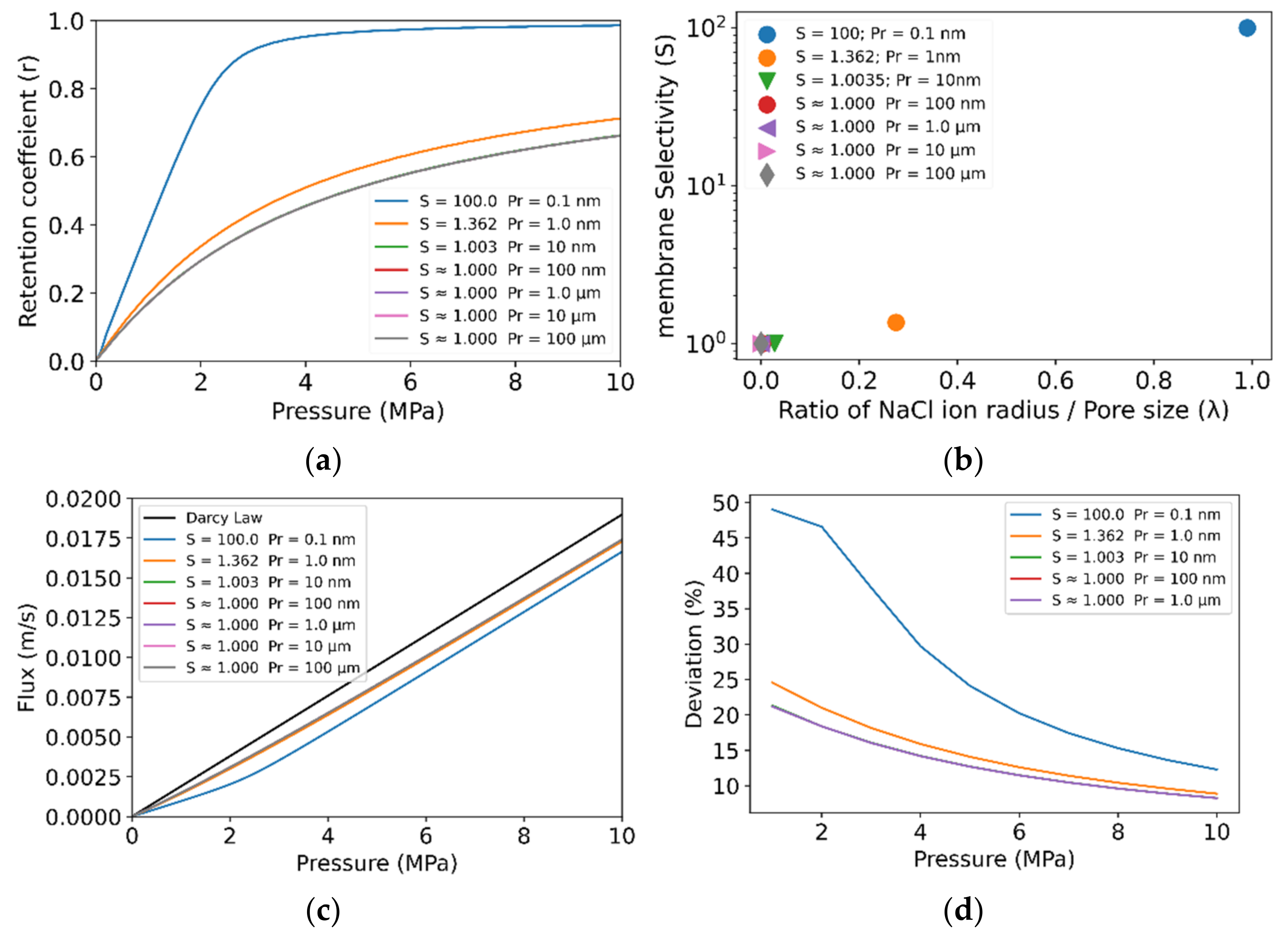
A sensitivity analysis of two parameters, the pore radius of Zone B and the bulk concentration ($c_b)$ were investigated to identify their influence on the relationship between the resultant flux and the pressure difference. A range of pore radii from the nanoscale to the macro scale was modelled (0.1 nm to 1mm). The parameters of the model are presented in Table 3. As presented in Equation (11), the retention coefficient of the low permeability zone depends on the selectivity coefficient $\left(S\right)$ and the ratio of the solute radius to the pore radius $\left(\lambda \right)$. The result from the simulation shows that the selectivity of the membrane increases sharply (approaches infinity) as the ratio of the solute radius to the pore radius $\left(\lambda \right)$ approaches unity (Figure 5a). At the given solute concentration, the selectivity coefficient for a pore radius of 10nm and above is approximately equal to unity $\left(\approx 1\right)$ (Figure 5b). The low permeable zones with a pore radius of the same magnitude as the solute radius have the highest selectivity coefficient $\left(S \approx 100 when r=0.99\right)$. The higher the value of $\lambda$, the higher the selectivity coefficient, and hence an increase in the deviation of the fluid flow from the Darcy law, as shown in Figure 5c,d. At a constant bulk solute concentration, it is easier for the solute molecules to move across the larger pores with no or little resistance.

Table 3. Parameters of the numerical model.

Parameter	Unit	Lower Limit	Upper Limit
Pore radius of Zone B	μm	$1.0\times {10}^{-4}$	100
Solute radius Na+, Cl− ions [65]	$\mathsf{\mu }\mathrm{m}$	$2.7\times {10}^{-4}$	$3.6\times {10}^{-4}$
$\mathrm{Selectivity} \mathrm{coefficient} \left(S\right)$ [18]		1	100
$\mathrm{Initial} \mathrm{concentration} \left(C0\right)$	$\mathrm{mol}/{\mathrm{m}}^3$	1	1000

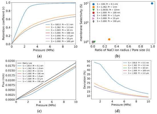
Figure 5. Effect of reverse osmosis on the resultant flow velocity at pore radii. $S$ is the selectivity coefficient and $Pr$ is the pore radius of zone B. (a) The membrane retention coefficient at different pore radii. (b) The ratio of solute to pore radius against selectivity of ultra-low permeability zone; (c) Darcy law with and without reverse osmosis. (d) Percentage deviation of simulated results from the Darcy law.

The percentage deviation from the Darcy law for the simulated pressure range and pore is between 8% and 49% (Figure 5d). The minimum deviation was recorded at the highest simulated pressure (10 MPa) and the highest simulated pore radius (100 $\mathsf{\mu }\mathrm{m}$), while the maximum deviation was recorded at the lowest simulated pressure (1 MPa) and the lowest pore radius (0.1 nm). For the given bulk concentration of NaCl, a pore radius above 10 nm, of the low permeable zone (zone B), does not increase the deviation from the Darcy law for all the simulated pressure ranges. Regardless, there is a significant deviation from the Darcy law for micron-scale and sub-micron pore radii.

Furthermore, the model was simulated at different bulk solvent concentrations while keeping the other parameters constant to determine the effect of the bulk fluid concentration on the possible deviation from the Darcy law. The range of simulated concentrations is between $\left(1 \mathrm{mol}/{\mathrm{m}}^3-1000 \mathrm{mol}/{\mathrm{m}}^3\right)$. The results for pore radii of 0.1 nm, 1 nm, and 100 μm are presented in Figure 6a–c, respectively. The results show that the deviation from the Darcy law increases with the increasing bulk solute concentration (Figure 6d). In addition, there is a pressure threshold (limiting pressure $\left(\Delta p_{lim}\right)$), above which there is linearity between the resultant flux and the pressure difference and below which there is non-linearity. The results presented in Figure 6d show that the bulk concentration is the dominant parameter that affects the resultant flux $\left(J_w\right)$ below the limiting pressure. In contrast, the pore radius is the dominant parameter that controls the deviation from the Darcy law above the limiting pressure.

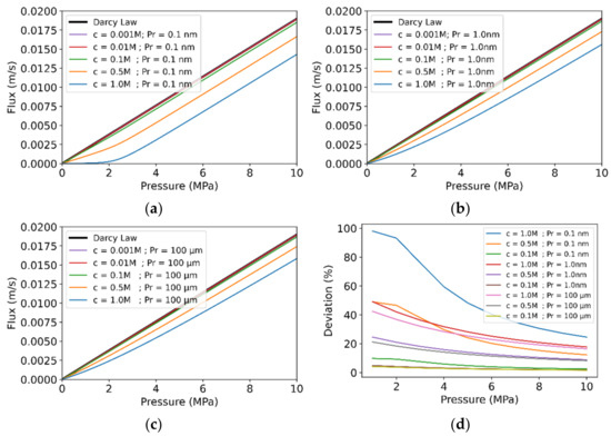
Figure 6. Effect of reverse osmosis on the resultant flow velocity at different solution concentrations and pore radii. $c$ is the bulk concentration, expressed in molarity (M); $Pr$ is the pore radius of zone B. (a) Pore radius = 0.1 nm, (b) pore radius = 1.0 nm, (c) pore radius = 100 µm, (d) percentage deviation of simulated results from the Darcy law.

3.3. Case-Study: Extent of Deviation from the Darcy Law for Different Tight/Shale Formations

A case study on tight oil and shale formations was investigated. The permeability and pore radius were taken from the literature. A summary of the characteristics of the different formations is presented in Table 4. The fluid density was determined using the Laliberte and Cooper correlation [66], and an average brine viscosity of 0.95 was used in the model [67].

Table 4. Parameters of the numerical model.

Formation	Permeabilty (mD) (Zone A and C)	Permeability (mD) (Zone B)	Pore Radius µm	NaCl Concentration (mol/m3)	Density (kg/m3)	Reference
Bakken	1	0.01	0.02	855.6	1034	[66,68,69,70]
Bazhenov	1	0.005	0.05	340	1013	[66,71]
Eagle Ford	1	$1.0\times {10}^{-6}$	0.009	500	1020	[66,72]

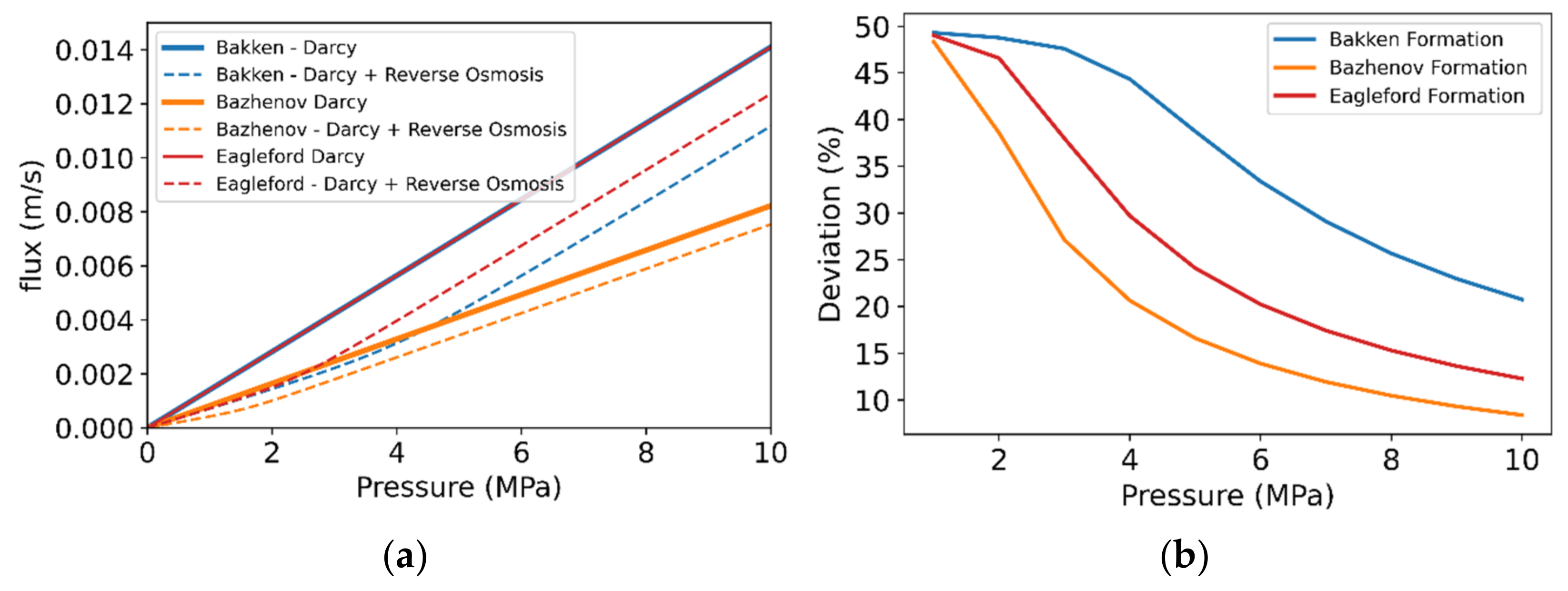
The results of the simulation of the different formations are presented in Figure 7a. The results show that the effect of reverse osmosis is significant at a low-pressure difference. At the lowest simulated pressure (1 MPa), all the formations recorded a significant deviation (approx. 49%) from the Darcy law (Figure 7b). Although the Eagle Ford formation was simulated with a lower pore and permeability for the zone B radius as compared to the Bakken formation, a higher value of deviation from the Darcy law was recorded due to the high concentration of the formation water of the Bakken formation $\left(855 \mathrm{mol}/{\mathrm{m}}^3\right)$. The Bazhenov formation presented the lowest deviation (8%) from the Darcy law at the highest simulated pressure due to the low concentration of formation water and the relatively higher pore radius of the low permeable zone.

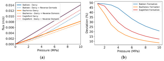
Figure 7. Effect of reverse osmosis on the resultant flow velocity for different tight oil/shale formations. (a) Resultant flow velocity proportionality to pressure difference with and without the effect of reverse osmosis. (b) Percentage deviation from the Darcy law for different tight oil formations.

This simple pore-scale model simulation has given insight into the extent of deviation from the Darcy law due to reverse osmosis. The range of 8% to 49% deviation from the Darcy law in a simple geometry is high enough to present an inaccurate estimation in reservoir models where the conditions for reverse osmosis are met, and the Darcy law is applied. The simulated parameters from the shale and tight reservoirs show that the limiting pressure for the various formations is 4 MPa, 1.6 MPa, and 2.6 MPa for the Bakken, Bazhenov, and Eagle Ford formations, respectively. In effect, below the limiting pressure, there is a non-linear proportionality between the resultant flux and the pressure difference. Estimating the resultant flux below the limiting pressure without considering the non-linear term between the fluid flux and the pressure difference will lead to over-predicting the resultant flux. Similarly, above the limiting pressure, where a linear proportionality between the fluid flux and the pressure drop is established, the Darcy equation still overestimates the fluid flux, as shown in Figure 7a. In the absence of a chemical potential gradient in the pore network, the extra term on the right-hand side of Equation (14) reduces to zero, and the equation becomes the classical Darcy law.

Furthermore, in processes such as high-salinity and low-salinity water flooding, where the injected brine has a different solute concentration than the in-situ reservoir brine, osmotic effects could be triggered and consequently result in the deviation of the flow from the classical Darcy law if only the hydraulic pressure drop $\left(\Delta p\right)$ is considered in the calculation [38,73]. As a result, it is vital that the chemical potential gradient be included in the Darcy equation to appropriately calculate the flow velocity and the limiting pressure threshold. When the chemical potential gradient decreases to zero, the equation becomes the conventional Darcy law.

To estimate the effect of the potential chemical gradient on the fluid flow, all other sub-micron mechanisms that influence fluid flow that have been reported in the literature were excluded from the model. While it is essential to include all previously documented sub-micron effects given in the literature, including all sub-micron effects into numerical reservoir simulators could lead to substantial computational costs. According to a study conducted by Yin et al., 2022 [74], the skeleton of the porous medium is critical in determining the dominant transport mechanisms at the sub-micron scale. This method could be useful for figuring out which parameters are the most important to include in numerical simulators.

4. Conclusions

This numerical study demonstrated how the emergence of chemical potential gradients caused by the selectivity features of sub-micron pores in tight and shale oil reservoirs causes a divergence from Darcy’s equation. The study has shown that introducing the chemical potential gradient to the right-hand side of the Darcy law in reservoir simulators will ensure the accurate estimation of the proportionality between the pressure difference and the fluid flux in sub-micron pores of tight and shale oil reservoirs.

The study presented the limiting pressure $\left(\Delta p_{lim}\right)$, below which the flow is non-linear due to the high effects of the chemical potential gradient and above which the flow is consistent with the Darcy law.

Despite the consistency of flow above the limiting pressure with the Darcy law, the resultant flux (flow velocity) is between 24% and 44% less than the flux, which would be obtained if only the conventional Darcy law were applied without the effect of a chemical potential gradient.

The characteristics of the shale and ultra-tight reservoirs simulated show that the threshold of the limiting pressure is up to 4 MPa. At the micron and sub-micron scale, the bulk brine concentration is the dominant parameter that influences the non-linearity of the curve below the limiting pressure, while the pore radius is the dominant parameter that influences the deviation from the Darcy law above the limiting pressure.

References

- Kundu, P.; Kumar, V.; Mishra, I.M. Experimental and numerical investigation of fluid flow hydrodynamics in porous media: Characterization of pre-Darcy, Darcy and non-Darcy flow regimes. Powder Technol. 2016, 303, 278–291. [Google Scholar] [CrossRef]
- Veyskarami, M.; Hassani, A.H.; Ghazanfari, M.H. Modeling of non-Darcy flow through anisotropic porous media: Role of pore space profiles. Chem. Eng. Sci. 2016, 151, 93–104. [Google Scholar] [CrossRef]
- Bratsun, D.; Siraev, R. Controlling mass transfer in a continuous-flow microreactor with a variable wall relief. Int. Commun. Heat Mass Transf. 2020, 113, 104522. [Google Scholar] [CrossRef]
- Sunjoto, S. The inventions technology on water resources to support environmental engineering based infrastructure. In Proceedings of the 5th International Conference on Education, Concept, and Application of Green Technology, Semarang, Indonesia, 5–6 October 2016; AIP Publishing LLC: Melville, NY, USA, 2017. [Google Scholar] [CrossRef]
- Satter, A.; Iqbal, G.M. Reservoir rock properties. In Reservoir Engineering; Elsevier: Amsterdam, The Netherlands, 2016; pp. 29–79. [Google Scholar] [CrossRef]
- Sun, S.; Zhang, T. Recent progress in multiscale and mesoscopic reservoir simulation. In Reservoir Simulations; Elsevier: Amsterdam, The Netherlands, 2020; pp. 205–258. [Google Scholar] [CrossRef]
- U.S. EIA. Annual Energy Outlook 2017 with Projections to 2050; Technical Report 8; EIA: Washington, DC, USA, 2017. [Google Scholar]
- Wang, S. Shale gas exploitation: Status, problems and prospect. Nat. Gas Ind. B 2018, 5, 60–74. [Google Scholar] [CrossRef]
- Yan, B.; Killough, J.E.; Wang, Y.; Cao, Y. Novel Approaches for the Simulation of Unconventional Reservoirs. In Proceedings of the Unconventional Resources Technology Conference, Denver, CO, USA, 12–14 August 2013. [Google Scholar] [CrossRef]
- Huang, Y.; Yang, Z.; He, Y.; Wang, X. An overview on nonlinear porous flow in low permeability porous media. Theor. Appl. Mech. Lett. 2013, 3, 022001. [Google Scholar] [CrossRef]
- Wang, D.; Wang, G. Dynamics of ion transport and electric double layer in single conical nanopores. J. Electroanal. Chem. 2016, 779, 39–46. [Google Scholar] [CrossRef]
- Wang, H.; Su, Y.; Wang, W.; Sheng, G.; Li, H.; Zafar, A. Enhanced water flow and apparent viscosity model considering wettability and shape effects. Fuel 2019, 253, 1351–1360. [Google Scholar] [CrossRef]
- Maknickas, A.; Skarbalius, G.; Džiugys, A.; Misiulis, E. Nano-scale water Poiseuille flow: MD computational experiment. In Proceedings of the AIP Conference Proceedings; AIP Publishing: Melville, NY, USA, 2020. [Google Scholar] [CrossRef]
- Yin, Y.; Qu, Z.; Zhu, C.; Zhang, J. Visualizing Gas Diffusion Behaviors in Three-Dimensional Nanoporous Media. Energy Fuels 2021, 35, 2075–2086. [Google Scholar] [CrossRef]
- Bai, B.; Zhu, R.; Wu, S.; Yang, W.; Gelb, J.; Gu, A.; Zhang, X.; Su, L. Multi-scale method of Nano(Micro)-CT study on microscopic pore structure of tight sandstone of Yanchang Formation, Ordos Basin. Pet. Explor. Dev. 2013, 40, 354–358. [Google Scholar] [CrossRef]
- Orlov, D.; Ebadi, M.; Muravleva, E.; Volkhonskiy, D.; Erofeev, A.; Savenkov, E.; Balashov, V.; Belozerov, B.; Krutko, V.; Yakimchuk, I.; et al. Different methods of permeability calculation in digital twins of tight sandstones. J. Nat. Gas Sci. Eng. 2021, 87, 103750. [Google Scholar] [CrossRef]
- Wyckoff, R.D.; Botset, H.G.; Muskat, M.; Reed, D.W. The Measurement of the Permeability of Porous Media for Homogeneous Fluids. Rev. Sci. Instrum. 1933, 4, 394–405. [Google Scholar] [CrossRef]
- King, F.H. Principles and Conditions of the Movements of Ground Water; US Government Printing Office: Washington, DC, USA, 1899; Volume 647.
- Churaev, N.V. Physical and Chemical Transport Processes in Porous Bodies.Pdf. 1990. Available online: https://www.studmed.ru/churaev-nv-fizikohimiya-processov-massoperenosa-v-poristyh-telah_b19eb202c34.html (accessed on 11 November 2021).
- Swartzendruber, D. Non-Darcy flow behavior in liquid-saturated porous media. J. Geophys. Res. 1962, 67, 5205–5213. [Google Scholar] [CrossRef]
- Dudgeon, C.R. An experimental study of the flow of water through coarse granular media. La Houille Blanche 1966, 52, 785–801. [Google Scholar] [CrossRef]
- Zeng, B.; Cheng, L.; Li, C. Low velocity non-linear flow in ultra-low permeability reservoir. J. Pet. Sci. Eng. 2011, 80, 1–6. [Google Scholar] [CrossRef]
- Lv, C.; Wang, J.; Sun, Z. An experimental study on starting pressure gradient of fluids flow in low permeability sandstone porous media. Pet. Explor. Dev. 2002, 29, 86–89. [Google Scholar]
- Han, X.; Wang, E.; Liu, Q. Non-Darcy flow of single-phase water through low permeability rock. J. Tsinghua Univ. 2004, 44, 804–807. [Google Scholar]
- Xu, S.; Yue, X.A. Experimental research on nonlinear flow characteristics at low velocity. J. China Univ. Pet. 2007, 31, 60–63. [Google Scholar]
- Xu, J.; Cheng, L.; Zhou, Y.; Ma, L. A new method for calculating kickoff pressure gradient in low permeability reservoirs. Pet. Explor. Dev. 2007, 34, 594. [Google Scholar]
- Siddiqui, F.; Soliman, M.Y.; House, W.; Ibragimov, A. Pre-Darcy flow revisited under experimental investigation. J. Anal. Sci. Technol. 2016, 7, 2. [Google Scholar] [CrossRef] [Green Version]
- Basak, P. Non-Darcy Flow and its Implications to Seepage Problems. J. Irrig. Drain. Div. 1977, 103, 459–473. [Google Scholar] [CrossRef]
- Soni, J.; Islam, N.; Basak, P. An experimental evaluation of non-Darcian flow in porous media. J. Hydrol. 1978, 38, 231–241. [Google Scholar] [CrossRef]
- Kececioglu, I.; Jiang, Y. Flow Through Porous Media of Packed Spheres Saturated with Water. J. Fluids Eng. 1994, 116, 164–170. [Google Scholar] [CrossRef]
- Klinkenberg, L. The Permeability of Porous Media to Liquids and Gases. API-41-200. All Days. 1941. Available online: https://faculty.ksu.edu.sa/sites/default/files/klinkenbergspaper-1941.pdf (accessed on 11 November 2021).
- Santoso, R.K.; Fauzi, I.; Hidayat, M.; Swadesi, B.; Aslam, B.M.; Marhaendrajana, T. Study of Non-Newtonian fluid flow in porous media at core scale using analytical approach. Geosyst. Eng. 2017, 21, 21–30. [Google Scholar] [CrossRef]
- Panfilov, M.; Fourar, M. Physical splitting of nonlinear effects in high-velocity stable flow through porous media. Adv. Water Resour. 2006, 29, 30–41. [Google Scholar] [CrossRef]
- Hayes, R.E.; Afacan, A.; Boulanger, B. An equation of motion for an incompressible Newtonian fluid in a packed bed. Transp. Porous Media 1995, 18, 185–198. [Google Scholar] [CrossRef]
- Whitaker, S. The equations of motion in porous media. Chem. Eng. Sci. 1966, 21, 291–300. [Google Scholar] [CrossRef]
- Crestel, E.; Kvasničková, A.; Santanach-Carreras, E.; Bibette, J.; Bremond, N. Motion of oil in water induced by osmosis in a confined system. Phys. Rev. Fluids 2020, 5, 104003. [Google Scholar] [CrossRef]
- Naeem, M.H.T.; Dehaghani, A.H.S. Evaluation of the performance of oil as a membrane during low-salinity water injection focusing on type and concentration of salts. J. Pet. Sci. Eng. 2020, 192, 107228. [Google Scholar] [CrossRef]
- Adler, P.M.; Malevich, A.E.; Mityushev, V.V. Nonlinear correction to Darcy’s law for channels with wavy walls. Acta Mech. 2013, 224, 1823–1848. [Google Scholar] [CrossRef]
- Javadi, M.; Sharifzadeh, M.; Shahriar, K.; Mehrjooei, M. Non-linear fluid flow through rough-walled fractures. In Proceedings of the ISRM Regional Symposium-EUROCK 2009, Cavtat, Croatia, 29–31 October 2009; OnePetro: Richardson, TX, USA, 2009. [Google Scholar]
- Qian, J.; Chen, Z.; Zhan, H.; Guan, H. Experimental study of the effect of roughness and Reynolds number on fluid flow in rough—Walled single fractures: A check of local cubic law. Hydrol. Processes 2010, 25, 614–622. [Google Scholar] [CrossRef]
- Kutiĺek, M. Non-Darcian Flow of Water in Soils—Laminar Region. Dev. Soil Sci. 1972, 2, 327–340. [Google Scholar] [CrossRef]
- Shannon, M.A.; Bohn, P.W.; Elimelech, M.; Georgiadis, J.G.; Mariñas, B.J.; Mayes, A.M. Science and technology for water purification in the coming decades. Nanosci. Technol. A Collect. Rev. Nat. J. 2008, 452, 301–310. [Google Scholar] [CrossRef] [PubMed]
- Greenlee, L.F.; Lawler, D.F.; Freeman, B.D.; Marrot, B.; Moulin, P. Reverse osmosis desalination: Water sources, technology, and today’s challenges. Water Res. 2009, 43, 2317–2348. [Google Scholar] [CrossRef] [PubMed]
- Li, D.; Wang, H. Recent developments in reverse osmosis desalination membranes. J. Mater. Chem. 2010, 20, 4551. [Google Scholar] [CrossRef]
- Shafi, H.Z.; Khan, Z.; Yang, R.; Gleason, K.K. Surface modification of reverse osmosis membranes with zwitterionic coating for improved resistance to fouling. Desalination 2015, 362, 93–103. [Google Scholar] [CrossRef]
- Whitworth, T.M. Clay membranes. In Encyclopedia of Earth Science; Kluwer Academic Publishers: Dordrecht, The Netherlands, 1999; pp. 83–85. [Google Scholar] [CrossRef]
- Hung, L.Y.; Lue, S.J.; You, J.H. Mass-transfer modeling of reverse-osmosis performance on 0.5–2% salty water. Desalination 2011, 265, 67–73. [Google Scholar] [CrossRef]
- Mai, Z.; Gui, S.; Fu, J.; Jiang, C.; Ortega, E.; Zhao, Y.; Tu, W.; Mickols, W.; der Bruggen, B.V. Activity-derived model for water and salt transport in reverse osmosis membranes: A combination of film theory and electrolyte theory. Desalination 2019, 469, 114094. [Google Scholar] [CrossRef]
- Fritz, S.J. Ideality of Clay Membranes in Osmotic Processes: A Review. Clays Clay Miner. 1986, 34, 214–223. [Google Scholar] [CrossRef]
- Kharaka, Y.K.; Berry, F.A. Simultaneous flow of water and solutes through geological membranes—I. Experimental investigation. Geochim. Et Cosmochim. Acta 1973, 37, 2577–2603. [Google Scholar] [CrossRef]
- Shackelford, C.D.; Meier, A.; Sample-Lord, K. Limiting membrane and diffusion behavior of a geosynthetic clay liner. Geotext. Geomembr. 2016, 44, 707–718. [Google Scholar] [CrossRef]
- Neuzil, C.E.; Person, M. Reexamining ultrafiltration and solute transport in groundwater. Water Resour. Res. 2017, 53, 4922–4941. [Google Scholar] [CrossRef]
- De Marsily, G. Stochastic Description of Flow in Porous Media. In Encyclopedia of Physical Science and Technology; Elsevier: Amsterdam, The Netherlands, 2003; pp. 95–104. [Google Scholar] [CrossRef]
- Gill, W.N.; Tien, C.; Zeh, D.W. Concentration Polarization Effects in a Reverse Osmosis System. Ind. Eng. Chem. Fundam. 1965, 4, 433–439. [Google Scholar] [CrossRef]
- Song, L.; Liu, C. A total salt balance model for concentration polarization in crossflow reverse osmosis channels with shear flow. J. Membr. Sci. 2012, 401–402, 313–322. [Google Scholar] [CrossRef]
- Liu, C.; Audra, M.; Ken, R.; Lianfa, S. Modeling of Concentration Polarization in a Reverse Osmosis Channel with Parabolic Crossflow. Water Environ. Res. 2014, 86, 56–62. [Google Scholar] [CrossRef]
- Gekas, V.; Hallström, B. Mass transfer in the membrane concentration polarization layer under turbulent cross flow. J. Membr. Sci. 1987, 30, 153–170. [Google Scholar] [CrossRef]
- Gherasim, C.V.; Cuhorka, J.; Mikulášek, P. Analysis of lead(II) retention from single salt and binary aqueous solutions by a polyamide nanofiltration membrane: Experimental results and modelling. J. Membr. Sci. 2013, 436, 132–144. [Google Scholar] [CrossRef]
- Hadi, S.; Mohammed, A.A.; Al-Jubouri, S.M.; Abd, M.F.; Majdi, H.S.; Alsalhy, Q.F.; Rashid, K.T.; Ibrahim, S.S.; Salih, I.K.; Figoli, A. Experimental and Theoretical Analysis of Lead Pb2 and Cd2 Retention from a Single Salt Using a Hollow Fiber PES Membrane. Membranes 2020, 10, 136. [Google Scholar] [CrossRef]
- Kim, S.; Hoek, E.M. Modeling concentration polarization in reverse osmosis processes. Desalination 2005, 186, 111–128. [Google Scholar] [CrossRef]
- Hassan, A.R.; Abdull, N.; Ismail, A.F. A Theoretical Approach on Membrane Characterization: The Deduction of Fine Structural Details of Asymmetric Nanofiltration Membranes. Desalination 2007, 206, 107–126. [Google Scholar] [CrossRef]
- Song, L. Thermodynamic modeling of solute transport through reverse osmosis membrane. Chem. Eng. Commun. 2000, 180, 145–167. [Google Scholar] [CrossRef]
- Safiddine, L.; Zafour, H.-Z.; Rao, U.M.; Fofana, I. Regeneration of Transformer Insulating Fluids Using Membrane Separation Technology. Energies 2019, 12, 368. [Google Scholar] [CrossRef]
- Renard, P.; de Marsily, G. Calculating equivalent permeability: A review. Adv. Water Resour. 1997, 20, 253–278. [Google Scholar] [CrossRef]
- Tanganov, B. About sizes of the hydrated salt ions—The components of sea water. Eur. J. Nat. Hist. 2013, 1, 36–37. [Google Scholar]
- Laliberté, M.; Cooper, W.E. Model for Calculating the Density of Aqueous Electrolyte Solutions. J. Chem. Amp Eng. Data 2004, 49, 1141–1151. [Google Scholar] [CrossRef]
- Zhang, H.-L.; Han, S.-J. Viscosity and Density of Water Sodium Chloride Potassium Chloride Solutions at 298.15 K. J. Chem. Amp Eng. Data 1996, 41, 516–520. [Google Scholar] [CrossRef]
- Hawthorne, S.B.; Jin, L.; Kurz, B.A.; Miller, D.J.; Grabanski, C.B.; Sorensen, J.A.; Pekot, L.J.; Bosshart, N.W.; Smith, S.A.; Burton-Kelly, M.E.; et al. Integrating Petrographic and Petrophysical Analyses with CO2 Permeation and Oil Extraction and Recovery in the Bakken Tight Oil Formation. In Proceedings of the SPE Unconventional Resources Conference, Calgary, AB, Canada, 16 February 2017. [Google Scholar] [CrossRef]
- Karimi, S.; Kazemi, H. Characterizing Pores and Pore-Scale Flow Properties in Middle Bakken Cores. SPE J. 2017, 23, 1343–1358. [Google Scholar] [CrossRef]
- Ramiro-Ramirez, S.; Flemings, P.B.; Bhandari, A.R.; Jimba, O.S. Steady-State Liquid Permeability Measurements in Samples from the Bakken Formation, Williston Basin, USA. In Proceedings of the SPE Annual Technical Conference and Exhibition, Dubai, UAE, 22 September 2021. [Google Scholar] [CrossRef]
- Karsanina, M.V.; Volkov, V.V.; Konarev, P.V.; Belokhin, V.S.; Bayuk, I.O.; Korost, D.V.; Gerke, K.M. Rapid Rock Nanoporosity Analysis Using Small Angle Scattering Fused with Imaging Data Based on Stochastic Reconstructions. In Proceedings of the SPE Russian Petroleum Technology Conference, Moscow, Russia, 22 October 2019. [Google Scholar] [CrossRef]
- Cho, Y.; Eker, E.; Uzun, I.; Yin, X.; Kazemi, H. Rock Characterization in Unconventional Reservoirs: A Comparative Study of Bakken, Eagle Ford, and Niobrara Formations. In SPE Low Perm Symposium; OnePetro: Richardson, TX, USA, 2016. [Google Scholar] [CrossRef]
- Yan, L.; Aslannejad, H.; Hassanizadeh, S.M.; Raoof, A. Impact of water salinity differential on a crude oil droplet constrained in a capillary: Pore-scale mechanisms. Fuel 2020, 274, 117798. [Google Scholar] [CrossRef]
- Yin, Y.; Qu, Z.; Prodanović, M.; Landry, C.J. Identifying the dominant transport mechanism in single nanoscale pores and 3D nanoporous media. Fundam. Res. 2022. [Google Scholar] [CrossRef]
Publisher’s Note: MDPI stays neutral with regard to jurisdictional claims in published maps and institutional affiliations. |
© 2022 by the authors. Licensee MDPI, Basel, Switzerland. This article is an open access article distributed under the terms and conditions of the Creative Commons Attribution (CC BY) license (https://creativecommons.org/licenses/by/4.0/).