
A Variable-Weather-Parameter MPPT Method Based on Equation Solution for Photovoltaic System with DC Bus

Abstract
:1. Introduction
- (1)
- A novel MPPT method is proposed by obtaining the real-time equation solutions of and . Meanwhile, it is unnecessary to solve the established equation set of the PV system with a DC bus at the MPP. Therefore, this MPPT method is very different from all existing VWP methods or other MPPT methods.
- (2)
- The real-time value of is first solved successfully by the obtained values of and . This work not only fills in the gap in obtaining the real-time equation solution of but also discloses the relationship between the bus voltage and other circuit parameters.
- (3)
- An implementation method for the ES-VWP method is successfully designed. This work is the first attempt to establish an equation set by sampling two operating points of a PV system at the same time.
- (4)
- In this work, the external data or measured values of the irradiance and temperature are no longer needed when an existing VWP method is implemented. Therefore, the lower hardware cost and better control independence can be achieved, which is beneficial to the widespread use of the VWP methods.
2. Principle
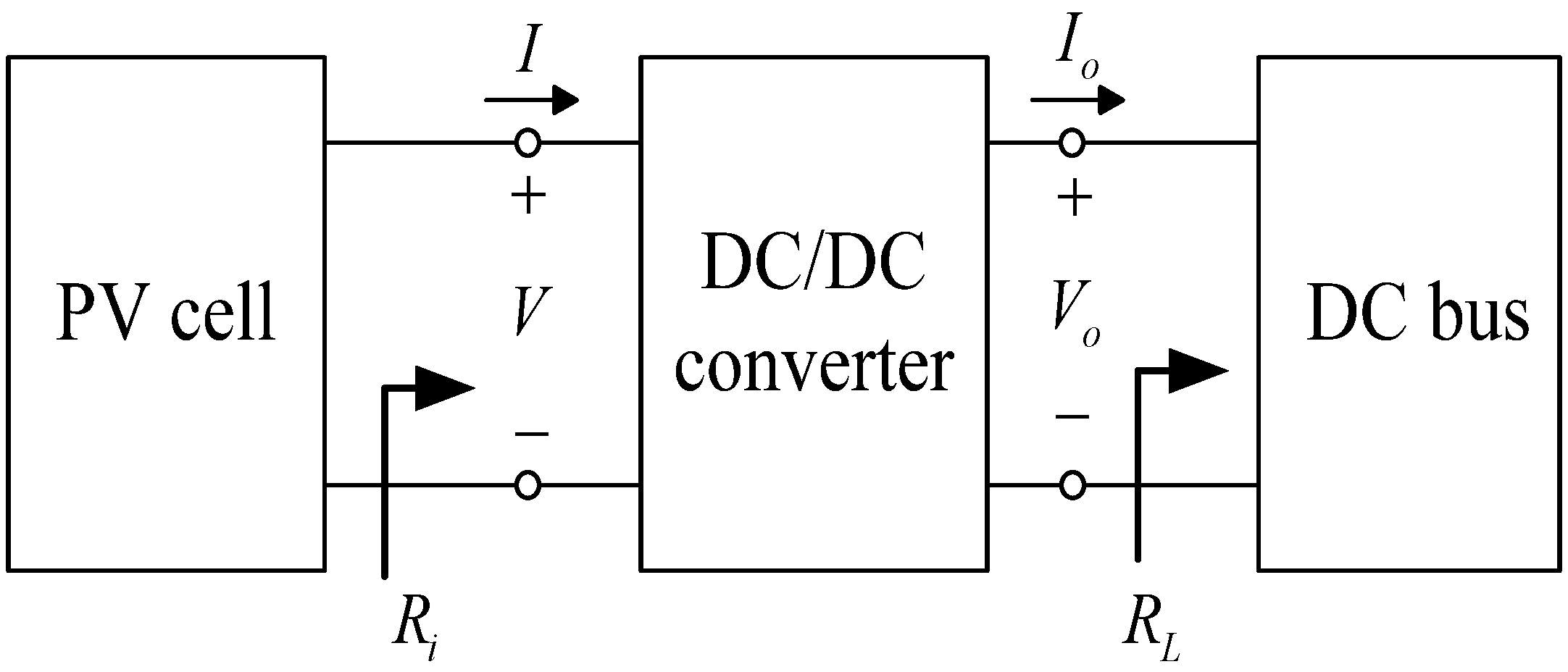
2.1. Mathematical Modeling of the PV System with a DC Bus
2.2. Establishment of the Equation Set
2.3. Equation Solution of the Bus Voltage
3. Proposition
4. Implementation
4.1. Design of System Configuration
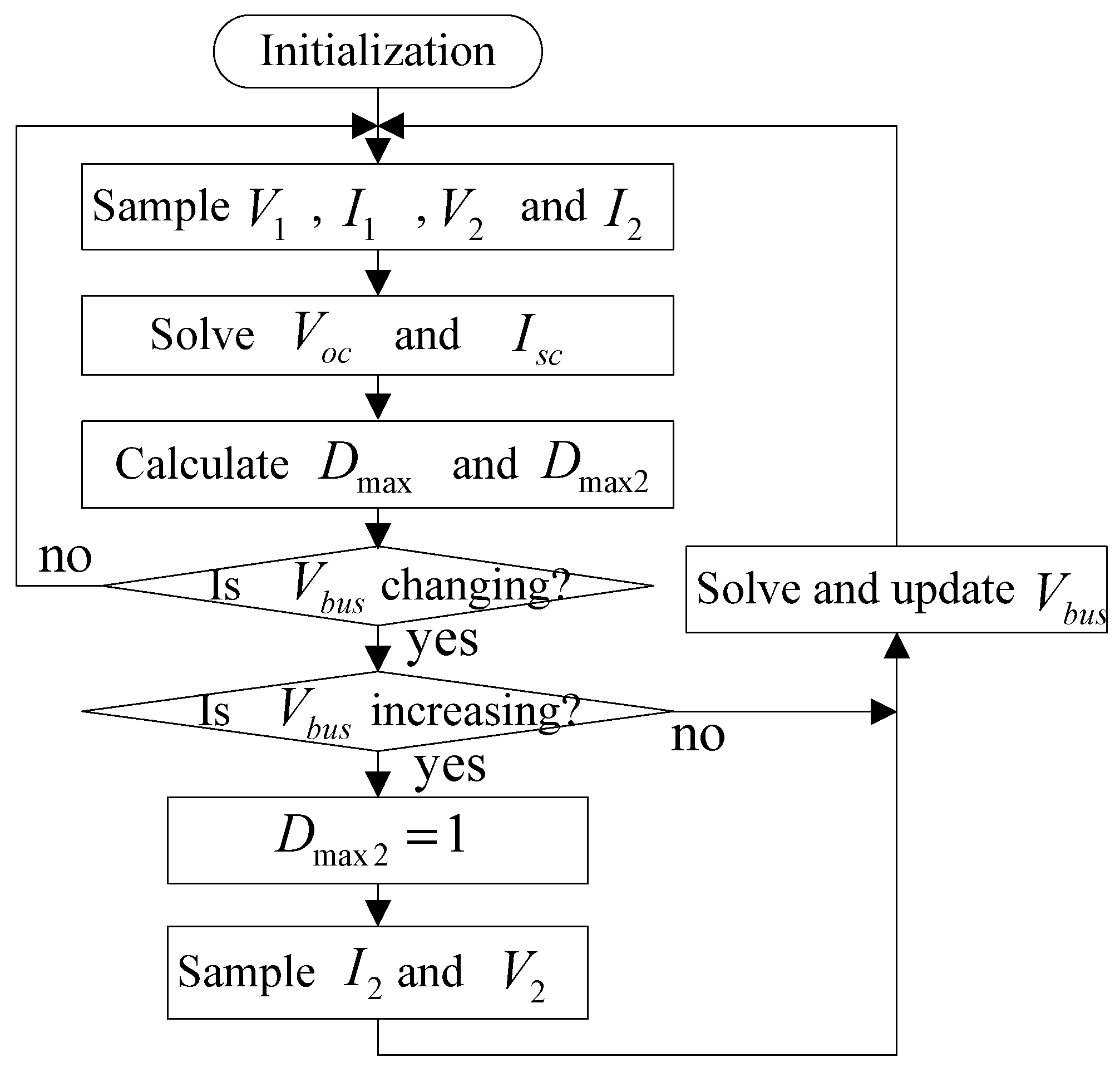
4.2. Design of the MPPT Control Process
5. Simulation Analysis
5.1. Feasibility and Availability of the Equation Solution
5.1.1. Verification and Acquisition of
5.1.2. Verification of Equation (19)
5.1.3. Verification of Equation (20)
5.2. Accuracy of the Equation Solution
5.2.1. Accuracy under Varying Weather Conditions
5.2.2. Influence of the Initial Value on the Accuracy
5.2.3. Influence of on the Accuracy
5.3. Feasibility and Availability of the Proposed Method
5.3.1. Analysis under Varying Conditions
5.3.2. Analysis under Varying Conditions
5.3.3. Analysis under Varying Conditions
5.4. MPPT Performance Comparison
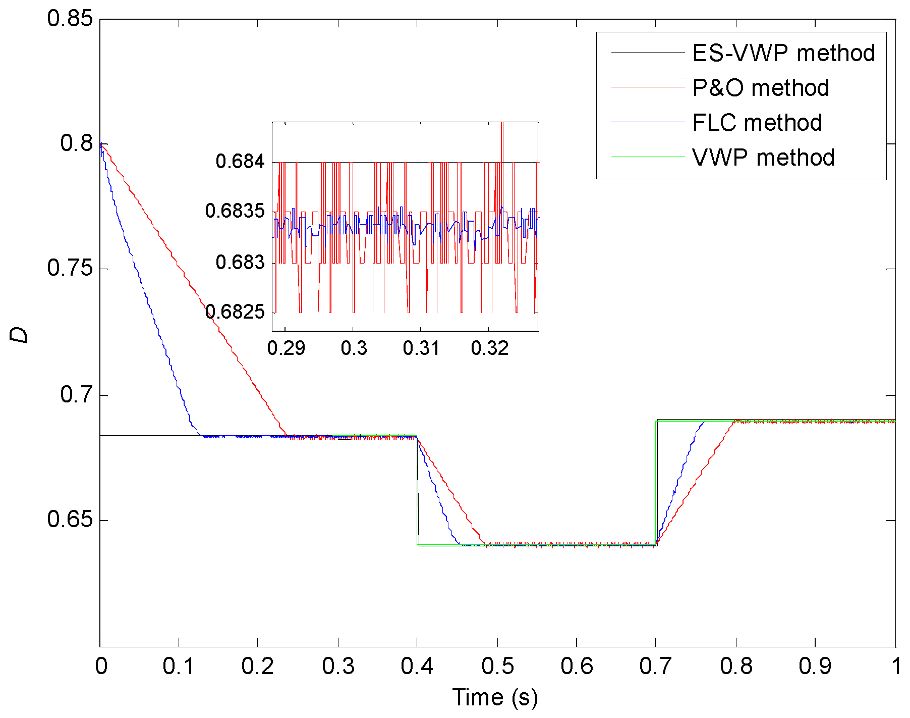
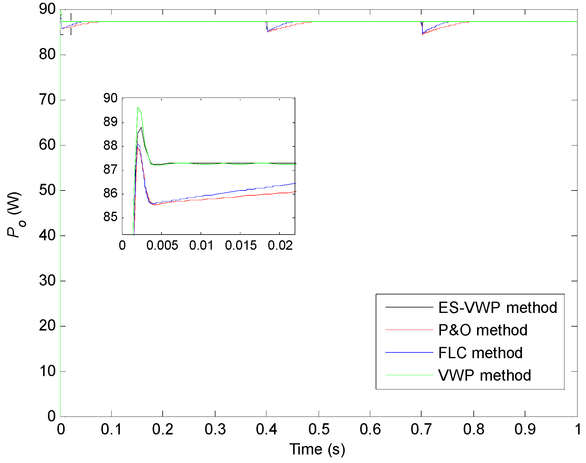
5.4.1. Performance under Varying Conditions
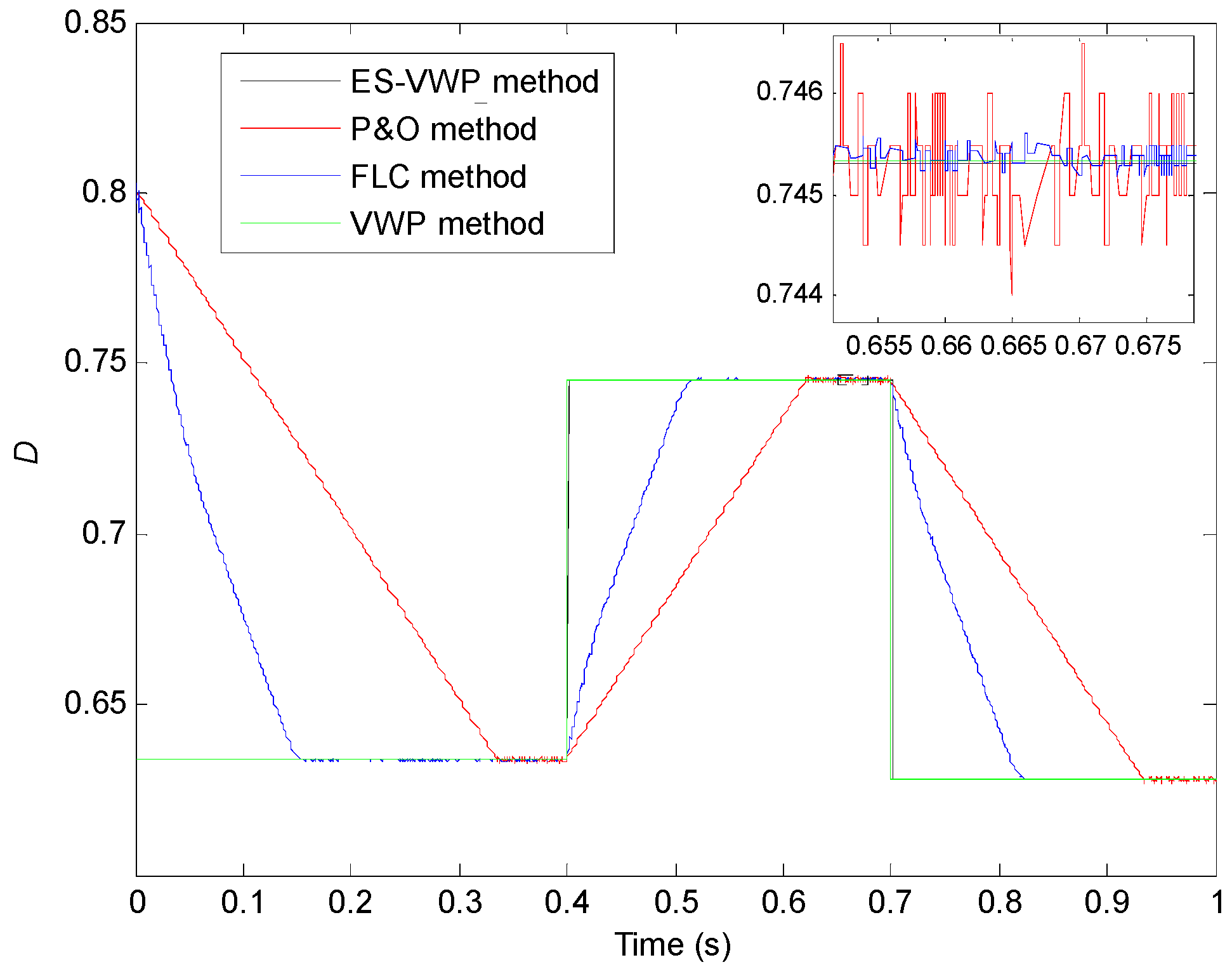
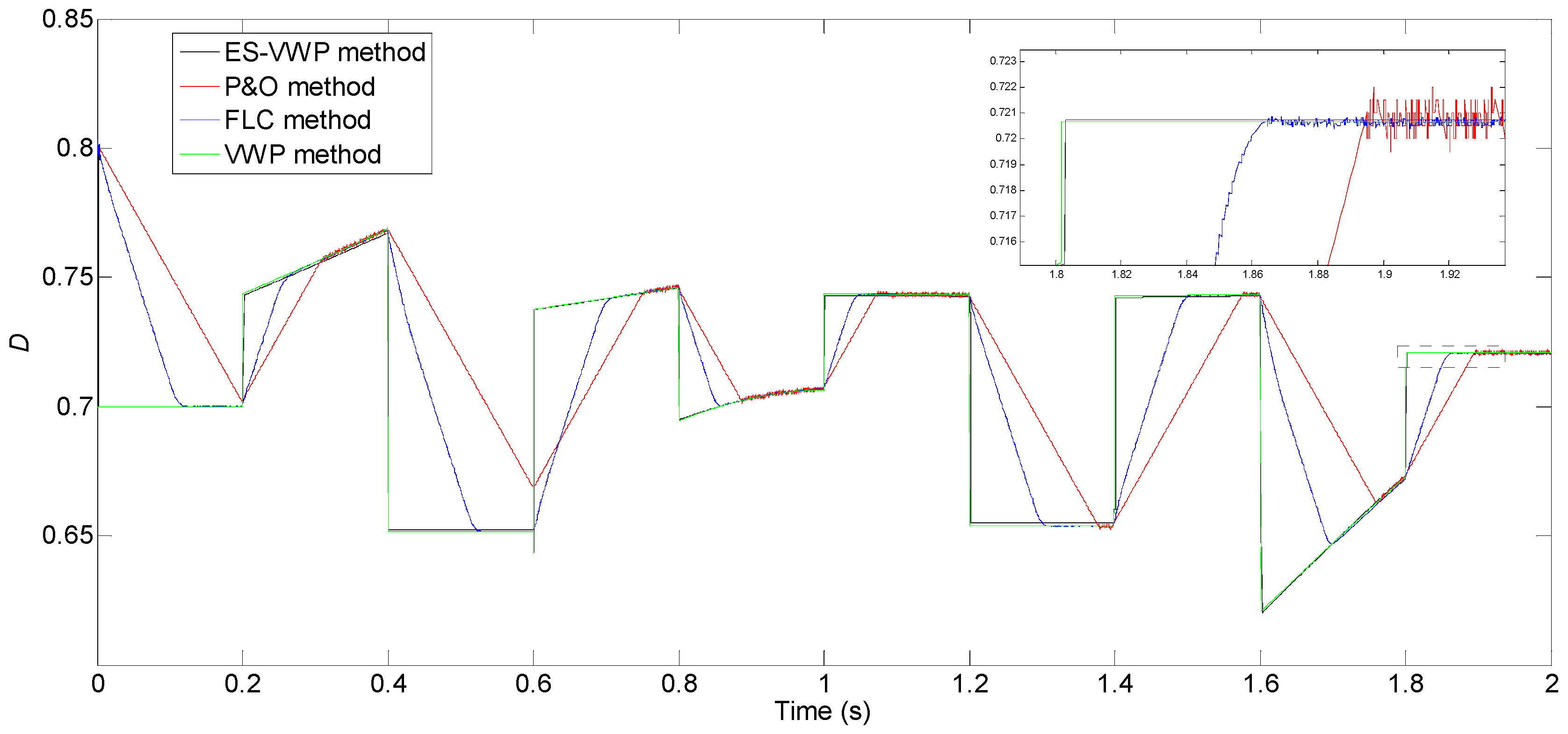
5.4.2. Performance under Varying Conditions
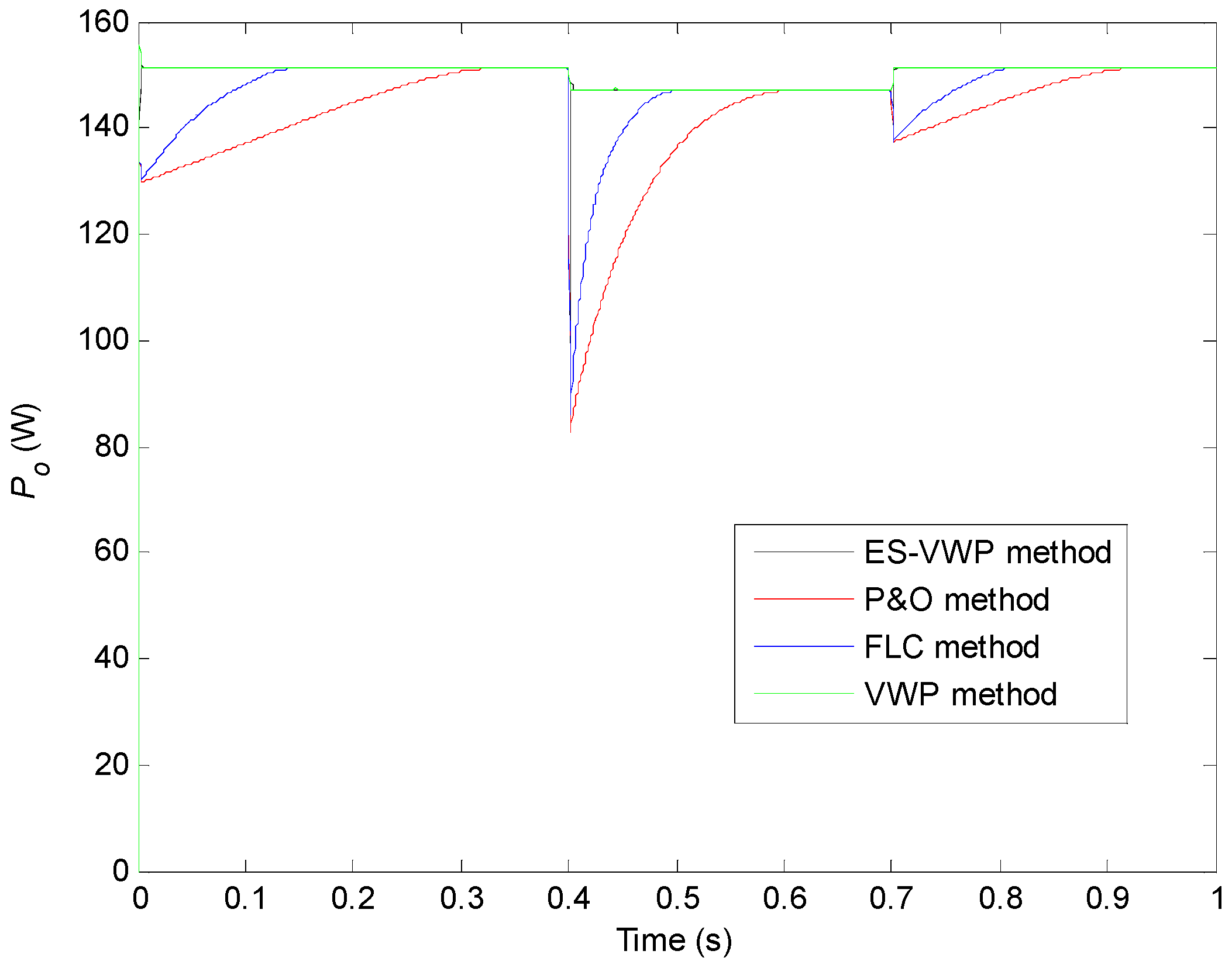
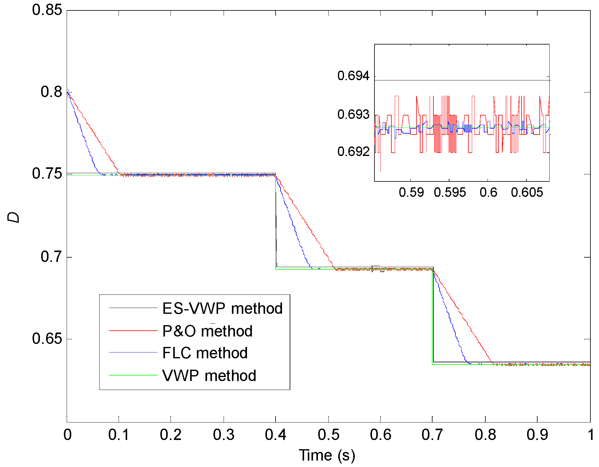
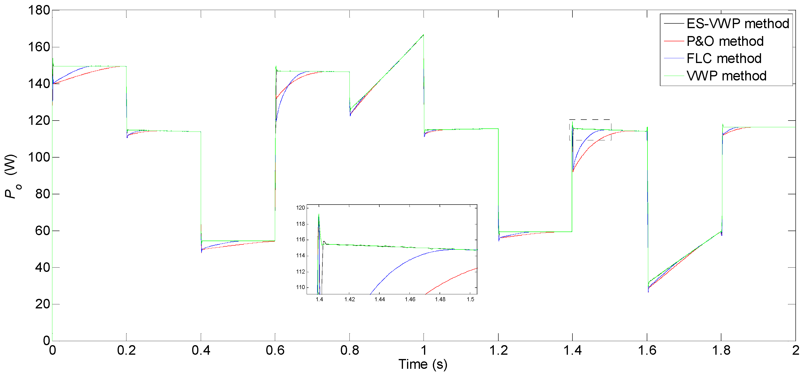
5.4.3. Performance under Varying Conditions
5.4.4. Performance under Arbitrary Conditions
6. Conclusions
Author Contributions
Funding
Acknowledgments
Conflicts of Interest
Nomenclature
| MPP | maximum power point | duty cycle of the PWM signal of the DDC | |
| MPPT | maximum power point tracking | solar irradiance | |
| ES-VWP | VWP MPPT method based on equation solution | cell temperature | |
| PV | photovoltaic | at the MPP | |
| PWM | pulse-width modulation | short circuit current of PV cell at STC | |
| P&O | perturbation and observation | MPP current of PV cell at STC | |
| INC | incremental conduction | open circuit voltage of PV cell at STC | |
| FLC | fuzzy logic control | MPP voltage of PV cell at STC | |
| SSO | salp-swarm optimization | output voltage of PV cell | |
| VWP | variable weather parameter | output current of PV cell | |
| SCC | short-circuit current | output voltage of the DDC | |
| I&T | irradiance and temperature | output current of the DDC | |
| AC | alternating current | load or equivalent load resistance of PV system | |
| DC | direct current | input resistance of the DDC | |
| STC | standard test conditions | output power of PV system | |
| DDC | DC/DC converter | voltage of the DC bus |
References
- Danandeh, M.A.; Mousavi, G.S.M. Comparative and comprehensive review of maximum power point tracking methods for PV cells. Renew. Sustain. Energy Rev. 2018, 82, 2743–2767. [Google Scholar] [CrossRef]
- Osmani, K.; Haddad, A.; Lemenand, T.; Castanier, B.; Ramadan, M. An investigation on maximum power extraction algorithms from PV systems with corresponding DC-DC converters. Energy 2021, 224, 120092. [Google Scholar] [CrossRef]
- Zhang, X.; Gamage, D.; Wang, B.; Ukil, A. Hybrid maximum power point tracking method based on iterative learning control and perturb & observe method. IEEE Trans. Sustain. Energy 2021, 12, 659–670. [Google Scholar]
- Danandeh, M.A.; Mousavi, G.S.M. A new architecture of INC-fuzzy hybrid method for tracking maximum power point in PV cells. Sol. Energy 2018, 171, 692–703. [Google Scholar] [CrossRef]
- Li, X.; Wen, H.; Hu, Y.; Jiang, L. A novel beta parameter based fuzzy-logic controller for photovoltaic MPPT application. Renew. Energy 2019, 130, 416–427. [Google Scholar] [CrossRef]
- Mirza, A.F.; Mansoor, M.; Ling, Q.; Yin, B.; Javed, M.Y. A Salp-Swarm Optimization based MPPT technique for harvesting maximum energy from PV systems under partial shading conditions. Energy Convers. Manag. 2020, 209, 112625. [Google Scholar] [CrossRef]
- Li, S. A variable-weather-parameter MPPT control strategy based on MPPT constraint conditions of PV system with inverter. Energy Convers. Manag. 2019, 197, 111873. [Google Scholar] [CrossRef]
- Li, S.; Ping, A.; Liu, Y.; Ma, X.; Li, C. A variable-weather-parameter MPPT method based on a defined characteristic resistance of photovoltaic cell. Sol. Energy 2020, 199, 673–684. [Google Scholar] [CrossRef]
- Eltawil, M.A.; Zhao, Z. MPPT techniques for photovoltaic applications. Renew. Sustain. Energy Rev. 2013, 25, 793–813. [Google Scholar] [CrossRef]
- Camilo, J.C.; Guedes, T.; Fernandes, D.A.; Melo, J.D.; Costa, F.F.; Sguarezi Filho, A.J. A maximum power point tracking for photovoltaic systems based on Monod equation. Renew. Energy 2019, 130, 428–438. [Google Scholar] [CrossRef]
- Xu, Y.; Kong, X.; Zeng, Y.; Tao, S.; Xiao, X. A modeling method for photovoltaic cells using explicit equations and optimization algorithm. Int. J. Electr. Power Energy Syst. 2014, 59, 23–28. [Google Scholar] [CrossRef]
- Li, S. A maximum power point tracking method with variable weather parameters based on input resistance for photovoltaic system. Energy Convers. Manag. 2015, 106, 290–299. [Google Scholar] [CrossRef]
- Sher, H.A.; Murtaza, A.F.; Noman, A.; Addoweesh, K.E.; Al-Haddad, K.; Chiaberge, M. A new sensorless hybrid MPPT algorithm based on fractional short-circuit current measurement and P&O MPPT. IEEE Trans. Sustain. Energy 2015, 6, 1426–1434. [Google Scholar]
- Li, S. A MPPT speed optimization strategy for photovoltaic system using VWP interval based on weather forecast. Optik 2019, 192, 162958. [Google Scholar] [CrossRef]
- Goud, J.S.; Kalpana, R.; Singh, B.; Kumar, S. A Global Maximum Power Point Tracking Technique of Partially Shaded Photovoltaic Systems for Constant Voltage Applications. IEEE Trans. Sustain. Energy 2019, 10, 1950–1959. [Google Scholar] [CrossRef]
- Valenciaga, F.; Inthamoussou, F.A. A novel PV-MPPT method based on a second order sliding mode gradient observer. Energy Convers. Manag. 2018, 176, 422–430. [Google Scholar] [CrossRef]
- Tousi, S.R.; Moradi, M.H.; Basir, N.S.; Nemati, M. A function-based maximum power point tracking method for photovoltaic systems. IEEE Trans. Power Electron. 2016, 31, 2120–2128. [Google Scholar] [CrossRef]
- Gerber, D.L.; Vossos, V.; Feng, W.; Marnay, C.; Nordman, B.; Brown, R. A simulation-based effificiency comparison of AC and DC power distribution networks in commercial buildings. Appl. Energy 2018, 210, 1167–1187. [Google Scholar] [CrossRef]
- Renaudineau, H.; Donatantonio, F.; Fontchastagner, J.; Petrone, G.; Spagnuolo, G.; Martin, J.P.; Pierfederici, S. A PSO-based global MPPT technique for distributed PV power generation. IEEE Trans. Ind. Electron. 2015, 62, 1047–1058. [Google Scholar] [CrossRef]
- Espinoza-Trejo, D.R.; Bárcenas-Bárcenas, E.; Campos-Delgado, D.U.; De Angelo, C.H. Voltage-oriented input-output linearization controller as maximum power point tracking technique for photovoltaic systems. IEEE Trans. Ind. Electron. 2015, 62, 3499–3507. [Google Scholar]
- Tang, L.; Wang, X.; Xu, W.; Mu, C.; Zhao, B. Maximum power point tracking strategy for photovoltaic system based on fuzzy information diffusion under partial shading conditions. Sol. Energy 2021, 220, 523–534. [Google Scholar] [CrossRef]
- Li, Q.; Zhao, S.; Wang, M.; Zou, Z.; Wang, B.; Chen, Q. An improved perturbation and observation maximum power point tracking algorithm based on a PV module four-parameter model for higher efficiency. Appl. Energy 2017, 195, 523–537. [Google Scholar] [CrossRef]
- Gopi, R.R.; Sreejith, S. Converter topologies in photovoltaic applications—A review. Renew. Sustain. Energy Rev. 2018, 94, 1–14. [Google Scholar] [CrossRef]
- Li, S.; Attou, A.; Yang, Y.; Geng, D. A maximum power point tracking control strategy with variable weather parameters for photovoltaic systems with DC bus. Renew. Energy 2015, 74, 478–488. [Google Scholar] [CrossRef]
- Li, S.; Li, Q.; Qi, W.; Chen, K.; Ai, Q.; Ma, X. Two variable-weather-parameter models and linear equivalent models expressed by them for photovoltaic cell. IEEE Access 2020, 8, 184885–184900. [Google Scholar] [CrossRef]
- Batarseh, M.G.; Za’ter, M.E. A MATLAB based comparative study between single and hybrid MPPT techniques for photovoltaic systems. Int. J. Renew. Energy Res. 2019, 9, 2023–2039. [Google Scholar]


| Operating Conditions | ① | ② | ③ | ④ | ⑤ | ⑥ |
|---|---|---|---|---|---|---|
| ) | variable | 1000 | variable | 1000 | variable | 1000 |
| 25 | variable | 25 | variable | 25 | variable | |
| 0.91 | 0.91 | variable | variable | 0.95 | 0.96 | |
| 0.001 | 0.001 | 0.001 | 0.001 | variable | variable | |
| 15 | 15 | 15 | 15 | 15 | 15 |
| (V) | (A) | (V) | (A) | (V) | (A) | (W) | (W) | ||||
|---|---|---|---|---|---|---|---|---|---|---|---|
| 300 | 17.8282 | 2.5233 | 17.8494 | 2.5203 | 21.9046 | 2.7570 | 0.8414 | 0.8404 | 44.9859 | 44.9855 | 0.8413 |
| 400 | 17.5772 | 3.3644 | 17.5777 | 3.3604 | 21.5716 | 3.6760 | 0.8544 | 0.8534 | 59.0694 | 59.0689 | 0.8543 |
| 500 | 17.3780 | 4.2055 | 17.3981 | 4.2006 | 21.3515 | 4.5950 | 0.8632 | 0.8622 | 73.0831 | 73.0825 | 0.8631 |
| 550 | 17.3237 | 4.6261 | 17.3438 | 4.6207 | 21.2849 | 5.0545 | 0.8659 | 0.8649 | 80.1406 | 80.1399 | 0.8658 |
| 600 | 17.2934 | 5.0466 | 17.3134 | 5.0407 | 21.2476 | 5.5140 | 0.8674 | 0.8664 | 87.2730 | 87.2723 | 0.8674 |
| 650 | 17.2871 | 5.4672 | 17.3071 | 5.4608 | 21.2398 | 5.9735 | 0.8677 | 0.8667 | 94.5113 | 94.5105 | 0.8677 |
| 700 | 17.3048 | 5.8877 | 17.3248 | 5.8809 | 21.2616 | 6.4330 | 0.8668 | 0.8658 | 101.8859 | 101.8850 | 0.8668 |
| 750 | 17.3466 | 6.3083 | 17.3666 | 6.3009 | 21.3129 | 6.8925 | 0.8647 | 0.8637 | 109.4266 | 109.4257 | 0.8647 |
| 800 | 17.4121 | 6.7288 | 17.4323 | 6.7209 | 21.3934 | 7.3520 | 0.8615 | 0.8605 | 117.1626 | 117.1616 | 0.8614 |
| 850 | 17.5016 | 7.1494 | 17.5216 | 7.1410 | 21.5028 | 7.8115 | 0.8571 | 0.8561 | 125.1220 | 125.1210 | 0.8571 |
| 900 | 17.6134 | 7.5699 | 17.6341 | 7.5610 | 21.6408 | 8.2710 | 0.8516 | 0.8506 | 133.3320 | 133.3309 | 0.8516 |
| 950 | 17.7485 | 7.9905 | 17.7695 | 7.9809 | 21.8067 | 8.7305 | 0.8451 | 0.8441 | 141.8182 | 141.8171 | 0.8451 |
| 1000 | 17.9057 | 8.4110 | 17.9271 | 8.4009 | 21.9999 | 9.1900 | 0.8377 | 0.8367 | 150.6052 | 150.6039 | 0.8377 |
| 1100 | 18.2846 | 9.2521 | 18.3069 | 9.2407 | 22.4654 | 10.1090 | 0.8204 | 0.8194 | 169.1709 | 169.1693 | 0.8203 |
| 1200 | 18.7445 | 10.0932 | 18.7680 | 10.0805 | 23.0304 | 11.0280 | 0.8002 | 0.7992 | 189.1922 | 189.1903 | 0.8002 |
| (V) | (A) | (V) | (A) | (V) | (A) | (W) | (W) | ||||
|---|---|---|---|---|---|---|---|---|---|---|---|
| −20 | 20.2263 | 7.4648 | 20.2536 | 7.4546 | 24.8511 | 8.1561 | 0.7416 | 0.7406 | 150.9847 | 150.9830 | 0.7416 |
| −10 | 19.7106 | 7.6750 | 19.7366 | 7.6649 | 24.2175 | 8.3859 | 0.7610 | 0.7600 | 151.2799 | 151.2783 | 0.7610 |
| 0 | 19.1949 | 7.8853 | 19.2195 | 7.8751 | 23.5839 | 8.6156 | 0.7815 | 0.7805 | 151.3582 | 151.3567 | 0.7814 |
| 5 | 18.9371 | 7.9905 | 18.9610 | 7.9803 | 23.2671 | 8.7305 | 0.7921 | 0.7911 | 151.3161 | 151.3146 | 0.7921 |
| 10 | 18.6793 | 8.0956 | 18.7025 | 8.0854 | 22.9503 | 8.8454 | 0.8030 | 0.8020 | 151.2197 | 151.2182 | 0.8030 |
| 15 | 18.4214 | 8.2007 | 18.4441 | 8.1906 | 22.6335 | 8.9602 | 0.8143 | 0.8133 | 151.0691 | 151.0677 | 0.8142 |
| 20 | 18.1636 | 8.3059 | 18.1856 | 8.2957 | 22.3167 | 9.0751 | 0.8258 | 0.8248 | 150.8643 | 150.8629 | 0.8258 |
| 25 | 17.9057 | 8.4110 | 17.9271 | 8.4009 | 21.9999 | 9.1900 | 0.8377 | 0.8367 | 150.6052 | 150.6039 | 0.8377 |
| 30 | 17.6479 | 8.5161 | 17.6687 | 8.5061 | 21.6831 | 9.3049 | 0.8500 | 0.8490 | 150.2920 | 150.2907 | 0.8499 |
| 35 | 17.3900 | 8.6213 | 17.4102 | 8.6112 | 21.3663 | 9.4197 | 0.8626 | 0.8616 | 149.9245 | 149.9232 | 0.8625 |
| 40 | 17.1322 | 8.7264 | 17.1518 | 8.7164 | 21.0495 | 9.5346 | 0.8755 | 0.8745 | 149.5027 | 149.5016 | 0.8755 |
| 45 | 16.8744 | 8.8316 | 16.8934 | 8.8216 | 20.7327 | 9.6495 | 0.8889 | 0.8879 | 149.0269 | 149.0257 | 0.8889 |
| 50 | 16.6165 | 8.9367 | 16.6349 | 8.9267 | 20.4159 | 9.7644 | 0.9027 | 0.9017 | 148.4967 | 148.4956 | 0.9027 |
| 55 | 16.3587 | 9.0418 | 16.3765 | 9.0319 | 20.0991 | 9.8792 | 0.9169 | 0.9159 | 147.9124 | 147.9113 | 0.9169 |
| 60 | 16.1008 | 9.1470 | 16.1181 | 9.1371 | 19.7823 | 9.9941 | 0.9316 | 0.9306 | 147.2738 | 147.2728 | 0.9316 |
(V) | (V) | (A) | (V) | (A) | (V) | (A) | (W) | (W) | |||
|---|---|---|---|---|---|---|---|---|---|---|---|
| 17 | 17.6628 | 6.6447 | 17.6812 | 6.6377 | 21.7015 | 7.2601 | 0.9625 | 0.9615 | 117.3641 | 117.3633 | 0.9624 |
| 16 | 17.6628 | 6.6447 | 17.6823 | 6.6373 | 21.7015 | 7.2601 | 0.9059 | 0.9049 | 117.3641 | 117.3632 | 0.9058 |
| 15 | 17.6628 | 6.6447 | 17.6836 | 6.6368 | 21.7015 | 7.2601 | 0.8492 | 0.8482 | 117.3641 | 117.3631 | 0.8492 |
| 14 | 17.6628 | 6.6447 | 17.6851 | 6.6362 | 21.7015 | 7.2601 | 0.7926 | 0.7916 | 117.3641 | 117.3629 | 0.7926 |
| 13 | 17.6628 | 6.6447 | 17.6869 | 6.6356 | 21.7015 | 7.2601 | 0.7360 | 0.7350 | 117.3641 | 117.3628 | 0.7360 |
| 12 | 17.6628 | 6.6447 | 17.6889 | 6.6348 | 21.7015 | 7.2601 | 0.6794 | 0.6784 | 117.3641 | 117.3625 | 0.6794 |
| 11 | 17.6628 | 6.6447 | 17.6912 | 6.6339 | 21.7015 | 7.2601 | 0.6228 | 0.6218 | 117.3641 | 117.3622 | 0.6228 |
| 10 | 17.6628 | 6.6447 | 17.6941 | 6.6328 | 21.7015 | 7.2601 | 0.5662 | 0.5652 | 117.3641 | 117.3618 | 0.5661 |
| Time Interval (s) | (W) | (W) | (W) | (W) | (W) | (ms) | (ms) | (ms) | (ms) | ||||||
|---|---|---|---|---|---|---|---|---|---|---|---|---|---|---|---|
| [0, 0.4] | 406 | 0.6840 | 0.6840 | 0.6835 | 0.6834 | 0.6835 | 59.91 | 59.91 | 59.91 | 59.91 | 59.91 | 5.4 | 220 | 118 | 6 |
| [0.4, 0.7] | 1202 | 0.6398 | 0.6398 | 0.6400 | 0.6402 | 0.6403 | 189.61 | 189.61 | 189.61 | 189.61 | 189.61 | 5.8 | 75 | 49 | 6 |
| [0.7, 1] | 498 | 0.6904 | 0.6904 | 0.6890 | 0.6894 | 0.6895 | 72.80 | 72.80 | 72.80 | 72.80 | 72.80 | 6 | 84 | 54 | 6 |
| Time Interval (s) | (W) | (W) | (W) | (W) | (W) | (ms) | (ms) | (ms) | (ms) | ||||||
|---|---|---|---|---|---|---|---|---|---|---|---|---|---|---|---|
| [0, 0.4] | 5 | 0.6337 | 0.6336 | 0.6336 | 0.6338 | 0.6336 | 151.32 | 151.31 | 151.32 | 151.32 | 151.32 | 5 | 330 | 148 | 6 |
| [0.4, 0.7] | 60 | 0.7453 | 0.7453 | 0.7455 | 0.7453 | 0.7453 | 147.28 | 147.27 | 147.28 | 147.27 | 147.28 | 6 | 210 | 110 | 6 |
| [0.7, 1] | 1.8 | 0.6282 | 0.6282 | 0.6280 | 0.6282 | 0.6282 | 151.35 | 151.34 | 151.35 | 151.35 | 151.35 | 5 | 225 | 121 | 5.5 |
| Time Interval (s) | (V) | (W) | (W) | (W) | (W) | (W) | (ms) | (ms) | (ms) | (ms) | |||||
|---|---|---|---|---|---|---|---|---|---|---|---|---|---|---|---|
| [0, 0.4] | 13 | 0.7517 | 0.7511 | 0.7498 | 0.7499 | 0.7498 | 87.27 | 87.27 | 87.27 | 87.27 | 87.27 | 8 | 96 | 55 | 12 |
| [0.4, 0.7] | 12 | 0.6939 | 0.6939 | 0.6925 | 0.6927 | 0.6927 | 87.27 | 87.27 | 87.27 | 87.27 | 87.27 | 7 | 108 | 62 | 9 |
| [0.7, 1] | 11 | 0.6361 | 0.6360 | 0.6345 | 0.6350 | 0.6350 | 87.27 | 87.27 | 87.27 | 87.27 | 87.27 | 6.5 | 110 | 65 | 11 |
Publisher’s Note: MDPI stays neutral with regard to jurisdictional claims in published maps and institutional affiliations. |
© 2022 by the authors. Licensee MDPI, Basel, Switzerland. This article is an open access article distributed under the terms and conditions of the Creative Commons Attribution (CC BY) license (https://creativecommons.org/licenses/by/4.0/).
Share and Cite
Li, S.; Chen, K.; Li, Q.; Ai, Q. A Variable-Weather-Parameter MPPT Method Based on Equation Solution for Photovoltaic System with DC Bus. Energies 2022, 15, 6671. https://doi.org/10.3390/en15186671
Li S, Chen K, Li Q, Ai Q. A Variable-Weather-Parameter MPPT Method Based on Equation Solution for Photovoltaic System with DC Bus. Energies. 2022; 15(18):6671. https://doi.org/10.3390/en15186671
Chicago/Turabian StyleLi, Shaowu, Kunyi Chen, Qin Li, and Qing Ai. 2022. "A Variable-Weather-Parameter MPPT Method Based on Equation Solution for Photovoltaic System with DC Bus" Energies 15, no. 18: 6671. https://doi.org/10.3390/en15186671
APA StyleLi, S., Chen, K., Li, Q., & Ai, Q. (2022). A Variable-Weather-Parameter MPPT Method Based on Equation Solution for Photovoltaic System with DC Bus. Energies, 15(18), 6671. https://doi.org/10.3390/en15186671