Abstract
A battery management system (BMS) is an important link between on-board power battery and electric vehicles. The BMS is used to collect, process, and store important information during the operation of a battery pack in real time. Due to the wide application of lithium-ion batteries in electric vehicles, the correct estimation of the state of charge (SOC) of lithium-ion batteries (LIBS) is of great importance in the battery management system. The SOC is used to reflect the remaining capacity of the battery, which is directly related to the efficiency of the power output and management of energy. In this paper, a new long short-term memory network with attention mechanism combined with Kalman filter is proposed to estimate the SOC of the Li-ion battery in the BMS. Several different dynamic driving plans are used for training and testing under different temperatures and initial errors, and the results show that the method is highly reliable for estimating the SOC of the Li-ion battery. The average root mean square error (RMSE) reaches 0.01492 for the US06 condition, 0.01205 for the federal urban driving scheme (FUDS) condition, and 0.00806 for the dynamic stress test (DST) condition. It is demonstrated that the proposed method is more reliable and robust, in terms of SOC estimation accuracy, compared with the traditional long short-term memory (LSTM) neural network, LSTM combined with attention mechanism, or LSTM combined with the Kalman filtering method.
1. Introduction
With the development of the automobile industry and accelerated urbanization, environmental issues and energy problems are becoming more and more concerning [1,2]. Traditional fuel cars are not friendly to the solution of environmental problems, due to the high emission of carbon monoxide, hydrocarbons, and some other solid particles that have adverse effects on human body [2]. On the other hand, as fuel is a non-renewable resource, with the current scale of fuel, fuel depletion will eventually come, and the automotive market must reduce fuel vehicles accordingly to reduce carbon emissions. Because of this, Norway will implement the policy of banning the sale of traditional fuel cars in 2025, and countries such as Germany, the UK, and France will also stop selling fuel cars between 2025 and 2040 one after another. Therefore, the development of electric vehicles has become a necessary direction and trend, and its rapid development will change all aspects of transportation and environmental issues [3]. Lithium batteries have a high energy density and low self-discharge rate; they are also characterized by relatively light weight, large storage capacity, no memory effect, and a long-life cycle [4], and they have been recognized as the main energy storage device for electric vehicles (EVs). However, because Li-ion battery packs operate in a highly dynamic driving environment, they will continue to deteriorate throughout the life cycle of the battery pack, thus affecting the performance of the BMS [5,6].
SOC indicates the remaining capacity of the battery, i.e., the percentage of the rated capacity remaining in the battery at a given discharge multiplier [7].
In this case, is the current charge of the battery, and is the calibrated capacity of the battery. SOC plays a pivotal role in the performance evaluation of a BMS system, and simultaneous and accurate dynamic SOC estimation has become an important part of the BMS system [6,8]. However, SOC cannot be measured directly; due to the highly non-linear and dynamic nature of the internal chemistry of Li-ion batteries [9], only indirect methods can be used to estimate the SOC of the battery. Therefore, dynamic yet accurate SOC estimation becomes a challenging task.
1.1. Literature Review
The current mainstream SOC algorithms are grouped into four categories, namely the open circuit voltage (OCV) [10], ampere-hour integral, model-based estimation, and data-based estimation methods.
The OCV method finds the corresponding SOC value by open-circuit voltage measurement based on the OCV–SOC mapping relationship [2,4,5,11]. The disadvantage is that OCV–SOC curve will become very sensitive in the middle of the discharge process, and a smaller change in OCV will cause a larger SOC error, and the OCV measurement needs to be left for a period of time to be measured, so it is difficult to achieve real-time SOC estimation [5,12].
The ampere-hour integral method is currently the most widely used algorithm for the SOC estimation of Li-ion batteries. It calculates the total power flowing into or out of the battery by integrating the current of the battery, as well as the current [11]. Although the ampere-hour integral method is relatively easy to calculate, the uncertainty of its initial power and instability of the discharge current lead to the low accuracy of SOC estimation, due to its open-loop estimation by nature.
Model-based estimation methods describe the external characteristics of the battery by combining different circuit elements to relate the SOC of the battery to variables, such as voltage and current [13]. In addition, circuit models are often combined with nonlinear observers, in order to achieve dynamic SOC estimation. The circuit model mainly includes the electrochemical model (EM) and equivalent circuit model (ECM) [14]. EM mainly responds to the internal chemical reaction mechanism of the battery, but it is difficult to determine all the parameters and has a large computational complexity. ECM is used with various battery components to depict the dynamic characteristics of the captured battery, and various ECM models have been proposed for lithium battery SOC estimation, including Rint [15], Thevenin, and partnership for new generation of vehicles (PNGV) models [15]. The model-based estimation methods that are widely used are mainly the Kalman filter (KF), particle filter (PF) [16], H infinity filter (HIF), other state observers, etc. Because of the highly nonlinear nature of the battery, Fengchun Sun et al. proposed an adaptive unscented Kalman filter (UKF) to estimate the battery SOC and approximate this highly nonlinear system [17]. Fei Zhang et al. proposed an H-infinity filter to estimate it in 2012 [18]. However, among these methods, building an accurate circuit model is the key to model-based estimation methods. For the complex and dynamic nonlinear system of lithium batteries, it is difficult to find a circuit model that can depict it completely accurately, thus resulting in a low applicability to SOC estimation.
In recent years, data-based estimation methods have been emerging in SOC estimation algorithms. The data-based estimation algorithm is used to measure a series of data, such as voltage, current, and temperature of the battery, and estimate the prediction of the SOC of the battery by one or more sets of measured data. Common data-based estimation methods include support vector machine (SVM), extreme learning machine (ELM), and neural network deep learning algorithms [19].
The SVM algorithm, first proposed by Cortes and Vapnik et al. In 1995 [20], maps the nonlinear sample features into higher dimensional feature vectors via kernel functions, thus resulting in a mapping relationship between the input variables and output SOC. In order to obtain the most suitable kernel function and parameters for the working conditions, the algorithm of particle swarm (PSO) was used to optimize the SVM by Ran Li et al. [21].
ELM was proposed by Guangbin Huang in 2004 [22], featuring that the weight values of the input and hidden layer connections and thresholds of the hidden layer can be randomized without subsequent processing adjustments. Jiani Du et al. applied ELM to the SOC estimation of batteries in 2013 [23].
Due to the rapid development of graphic processing units (GPU) in recent years, the training speed of neural networks has been reduced from months to days and hours or even minutes. Thanks to this, neural networks and SOC estimation methods for deep learning have also emerged. A neural network can be considered a black box, in which a large number of nonlinear functions are stored, which are nonlinear and can learn various deep, as well as abstract, features [24]. In battery SOC estimation, the input data of the battery is sampled, processed for analysis, and passed into the neural network. According to the powerful learning ability of the neural network, a set of suitable neural network parameters can be trained to fit the final SOC output value that needs to be obtained, and the method does not require a tedious and complicated battery modeling process; as long as the data input to the network is large and accurate enough [25], the SOC estimation is robust for all different battery situations.
The neural networks in SOC estimation are wavelet neural network (WNN), back propagation neural network (BP) trained by error backpropagation, etc. Bizhong Xia et al. proposed a multi-hidden layer WNN model optimized by the L-M algorithm to estimate SOC in 2018 [26]; in the same year, Hannan, MA et al. proposed to improve BP network using BSA algorithm [27].
Since the battery charging and discharging process is continuous, and the sampling of the battery data is also continuous, SOC estimation can be considered as a time-series regression prediction problem. In traditional neural networks, signals are not passed between neurons at the same level, which leads to a problem, i.e., that the output signal is only related to the input signal, but not to the backward and forward relationship or sequence of the input signal. If the overall network lacks a “memory” function, then a “memory” network with the ability to understand the before and after information or the temporal order of data is needed. Based on this, recurrent neural networks (RNN) were introduced, and Hicham Chaoui et al. proposed estimating the SOC using RNN in 2017 [28].
RNN use the internal circulation of neural networks to preserve the connection of the contextual information of the time series; however, in practical applications, temporal information tends to decay because the transmission interval is too long. Therefore, ordinary RNN do not have a good way to deal with the long-term dependence problem of temporal information; in addition, RNN produce a series of gradient vanishing problems when back-propagating. To solve these, LSTM was proposed by Hochreiter, S and Schmidhuber, J in 1997 [29], which can learn the long-term dependence problem of information, and LSTM has achieved great success in natural language processing (NLP), as well as temporal data processing [30]. Fangfang Yang et al. successfully applied LSTM network applied to battery SOC estimation, which produced better results [31].
Gated recurrent unit (GRU) is a variant of LSTM, which was proposed by K. Cho in 2014. GRU uses two gates to regulate the flow of long-term information, as well as forgetting with fewer parameters and faster training, compared to LSTM. Meng Jiao et al. proposed GRU-RNN in 2020 to estimate the SOC of the battery [32].
Although LSTM has a good effect on battery SOC estimation, it cannot do a very accurate estimation of battery SOC under various battery temperatures and operating conditions, due to the dynamic nature of battery operation. Fangfang Yang et al. proposed a method combining LSTM and UKF [33], and Yong Tian et al. proposed combining LSTM with an adaptive cubature Kalman filter (ACKF) [4], which greatly improved the estimation accuracy. However, since the results of the filtering algorithm partly depend on the output of the network, the ups and downs of the network output results will lead to a large impact on the final filtering results. Therefore, a stable network output under different battery conditions becomes an indispensable part.
1.2. Contributions of the Work
In order to solve the above series of problems, this paper proposes a method combining machine learning and traditional filtering to estimate the SOC of lithium batteries, i.e., LSTM–attention combined with Kalman filtering. First, for the characteristics of the internal nonlinearity of the battery and SOC estimation as a time series problem, an LSTM network was designed through the collected battery voltage, current, and temperature data, combined with the attention mechanism to assign weights to each time step and according to the assigned weight scores, in order to decide which time step input data information; it will be more useful for training, so as to roughly estimate the SOC. In addition, Kalman filtering was used to improve the accuracy of the predicted SOC values, reduce the prediction error, and smooth the prediction output. Then, data from different dynamic driving cycles were used to evaluate the performance of the method. The contributions of this work are mainly as follows.
- An LSTM–attention model for SOC estimation is proposed. The attention mechanism was used to optimize the LSTM network, so that the network can capture deeper input–output mapping relationships, as well as the importance of timing information, and it was experimentally demonstrated that the optimized network converges faster and smoother, in terms of loss values during training and testing, to ensure the accuracy of SOC estimation.
- Kalman filtering was used to update the prediction results. The estimation accuracy of the SOC was further improved, so that the estimation results of the proposed network can be smoother and have less error.
- The effects of different initial power, temperature, and operating conditions on the model accuracy were analyzed experimentally. In addition, the system model in this paper was compared with the existing LSTM and LSTM, combined with the Kalman filter, and the effectiveness of the LSTM–attention–Kalman method for SOC estimation was verified using a public data set.
1.3. Organization of This Article
The remainder of this paper is organized as follows. Section 1 introduces the principles of long short-term memory networks. Section 2 describes the network structure and the application of the attention mechanism on LSTM. Section 3 details the Kalman filtering method and how it is applied on top of the output results of the network. Section 4 summarizes the sources of the data and the normalized processing of the data. Section 5 is used to conduct comparative experiments and record the results. Finally, Section 6 is used to conclude the whole work.
2. Hybrid Network Construction
2.1. Neural Network SOC Model
RNN were compared to the ordinary fully connected neural network. The hidden layer structure was added, and the hidden layer was used to keep the history information. Figure 1 shows the refined structure of a hidden layer unit.
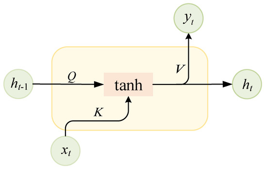
Figure 1.
RNN hidden layer cell structure diagram.
Where is the input vector of the network at moment , and is the hidden layer state vector at the previous moment, which contains the memory information of the previous moment. are the weight matrices shared by the parameters, and tanh is the chosen activation function. is the hidden layer state at the current moment, and denotes the output at the moment , which is expressed as follows.
LSTM uses gate structure to control the circulation and loss of features, which is a good solution to the problems of gradient explosion, gradient disappearance, and long-term dependence in traditional RNN. The three gates in LSTM are the forgetting, input, and output gates. Figure 2 shows the structure of an LSTM cell.
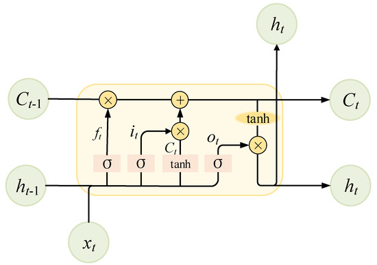
Figure 2.
LSTM cell structure diagram.
Where the forgetting gate of the LSTM is used to control which information is forgotten, and it determines the value of the output vector by the input information at the current moment, as well as the state information at the previous moment. The size of determines the importance of the output information—0 is to discard all the ingested information, and 1 is to keep all the information. The expression of is as follows.
The input gates of the LSTM are used to control the information added by the cells. and control the updated information through the input gates, and is described as follows.
Next, the updates of the candidate cellular information are filtered by , as well as , through an activation function layer tanh. The expression of is shown as follows.
Then comes the part of the update gating, where the output is determined by the cell information of the current moment and the cell state information of the previous moment output by the forgetting gate, plus the candidate information of the cell and updated information.
Finally, and obtain a condition to determine the cell state characteristics through the sigmoid layer, and then the state information is passed through the tanh layer to obtain a vector between −1 and 1. The final output information is obtained by multiplying the cell state characteristics condition with the obtained vector. The step is represented as follows.
This is where and are the weights and deviations of the network, respectively.
2.2. Attentional Mechanisms
In this paper, a “many-to-one” sliding window was designed to enable the LSTM network to make better use of the information of each time step of various working conditions data, combined with the attention mechanism for training. The sliding window is shown in Figure 3. The choice of the window size required some consideration, too large a window is not conducive to fully and continuously predicting the data at all historical moments in real time, while too small a window does not fully utilize the historical information of the data and, thus, does not allow the attention mechanism to be better applied at each time step. Based on the experiment, the sliding window size chosen is 50. In this paper, the input is defined as , where , , and are all the voltage, current, and temperature data within a sliding window of 50 moments, respectively. The corresponding label is chosen as , which is denoted as the SOC value at the next moment.
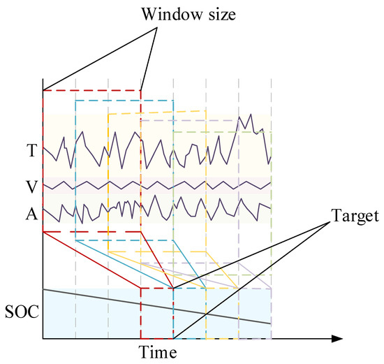
Figure 3.
Sliding window diagram.
The use of the attention mechanism allows the model to capture more direct dependencies at different points in time. In this paper, LSTM is used as the base model that can generate hidden states . The structure of the attention model is shown in Figure 4.
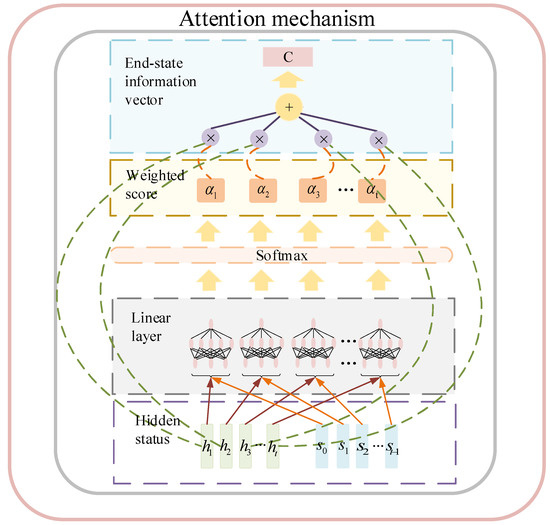
Figure 4.
Attention mechanism structure.
It is possible to compute a final state information vector to be used to act on the up and down time points. These vectors of up and down time points can be used to compute a new state sequence vector , where can be expressed as follows.
where is the length of the chosen time step, specifically chosen here as 50. The state sequence vector is determined by , , and the output of the model at moment t − 1. is the weight parameter of the model, and is the hidden state of the model. is calculated as shown below.
where is a specific function. It can take many forms; here, a specific linear layer of the neural network was chosen to capture the information, and then we chose the Softmax function to normalize the captured parameters to calculate the weight parameter for better utilization of the network. The size of is related to the sequence of states and at the previous moment.
Then, the hidden state and probability vector are obtained for each time point, and the dot product sum of the two at each time node in each time step, i.e., the final vector that can link the information of the upper and lower time points is obtained.
In traditional LSTM, each hidden layer has the same impact on the prediction target when dealing with time-series data. This results in a similar impact on the final label, whether it is the charging process, resting process, or cross-current discharge of the battery; however, with the fusion of attention mechanisms, the model can more accurately distinguish which data are more “useful” and which data are relatively “less important”. The contribution of each hidden layer to the output will be differentiated, so that the training loss function is smaller and convergence is faster. In this paper, the overall structure of LSTM + attention was established, as shown in Figure 5. built from a sliding window was used as input, passed through the LSTM + attention layer, and then followed by a linear layer; finally, the output layer was used for regression.
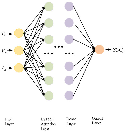
Figure 5.
Overall network structure diagram.
The number of nodes of the designed network LSTM has a great influence on the network parameters—too few nodes will make the training RMSE high, while too many nodes will make the network have a tendency to overfit. Here, 128 nodes were chosen; in addition, we tried 256 nodes, but the network performance did not improve significantly. In order to make the network weights lower, this value was finally determined. Too large an epoch is not beneficial for model fitting and time saving, and too large a batch size leads to a decrease in model generalization ability. It was observed that, after 200 calendar hours, the training loss leveled off and fluctuated slightly above and below a stable value. The batch size of 64 and 200 epochs were chosen, considering the time efficiency and accuracy of the model. The loss function evaluated at the end of each forward propagation during training was chosen as the mean squared error (MSE), which is given by the following Equation.
where is the true value of the SOC output at moment t, and is the network output at moment t. is the overall length of the time-series data. The training of each network batch is divided into two processes, i.e., forward propagation and backward transmission. The forward pass causes the network to generate an estimate at the end of each time step, and the back propagation minimizes the error between this estimate and the true value, according to the gradient of the loss function, thus updating the network weight parameters. Here Adam is chosen as the optimizer, which can further update the variables based on the previous gradient oscillations.
In addition, a conventional LSTM network was selected for comparison experiments, keeping the number of parameters, batch size, epoch, input data, and random number seeds unchanged.
In this paper, data from three driving schedules trained on LSTM + attention and LSTM were compared for US06, DST, and FUDS, respectively, where US06 simulates the car under high acceleration and DST satisfies the average characteristics and only seven discrete power levels, which is a simplification of the actual load conditions of the battery; its working condition discharge current curve is correspondingly simple. FUDS simulates the driving conditions of electric vehicles operating in the city. The loss values of the loss function for each epoch during training are shown in Figure 6 below.
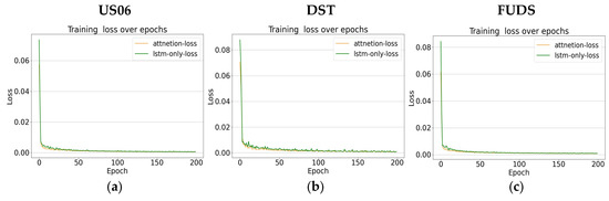
Figure 6.
Comparison of loss values during training: (a) US06 condition; (b) DST condition; (c) FUDS condition.
The partial losses for the US06 condition are enlarged and shown in Figure 7, which shows that, whether it is the final loss value, convergence speed during training, or smoothness of the curve during training, a large number of experiments showed that the addition of the attention mechanism performs better than the original LSTM.
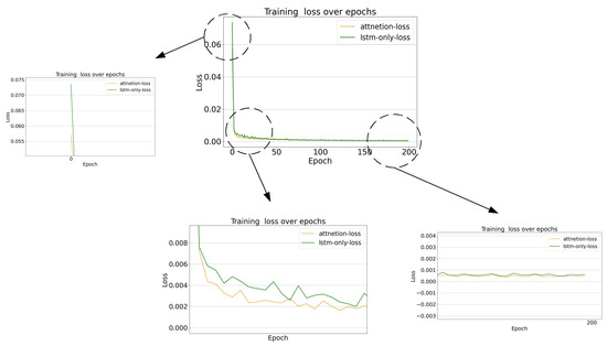
Figure 7.
US06 working condition training process loss value amplification.
The specific SOC test results of the combined attention model, compared with the LSTM model; their corresponding combined Kalman algorithm will be provided in the subsequent sections and will not be repeated here.
3. Kalman Filter
In this section, Kalman algorithm is used to improve the output results of the attention network. It allows the optimal estimation of the state of the system by using the data from the input and output observations of the system. In addition, in this process, the noise, including the system, can also be filtered out and does not need to meet the condition that both the signal and noise are smooth; therefore, it is widely used in various fields.
Kalman filtering is a recursive estimation built on the hidden Markov model. Its dynamical system can be represented by a Markov chain built on a linear operator that satisfies a normal distribution of disturbances, and this linear operator increases with time to produce a new state.
In order to estimate the internal state of the observed process from a series of noisy observations using the Kalman filter, the process must be modeled in the framework of the Kalman filter. This means that for each moment of , the matrix , , , , and is defined separately.
The Kalman model assumes that the real state at time evolves from the previous moment, that is, time . The state vector can be represented by the following equation.
The above equation is called the equation of state, where is the state transformation matrix acting on . is the state control matrix acting on the state control vector . is the noise satisfying a Gaussian distribution with mean 0. ~ . is the system noise covariance matrix.
For the measurement vector of at the moment .
The above equation is called the measurement equation. In this, is the observation matrix. It is used to map the real state space into the observed space. is the noise of Gaussian distribution with mean 0. is its covariance matrix, which satisfies ~ .
The operation of Kalman’s algorithm consists of two steps: predict and update, respectively. The prediction phase filter can use the estimation result of the previous moment to estimate the state of the current moment. The update filter optimizes the predict value with the current state observation. This is used to make the estimates more accurate.
Figure 8 shows the flow chart of Kalman’s algorithm.
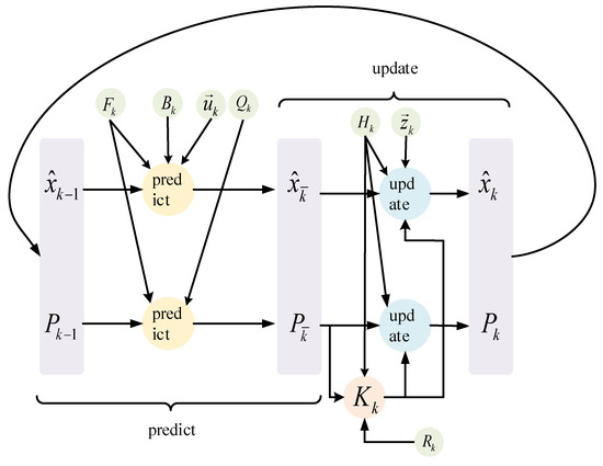
Figure 8.
Kalman algorithm process.
In the prediction phase, since the optimal state of the system at time obeys a Gaussian distribution:
According to the prediction equation of Equation (13), the predicted state at the moment of can be obtained as:
The predicted state at the moment of is obtained:
is the posterior estimation state at the moment . Similarly, is the posterior estimation state at the moment . is the state of the prior estimate at the moment . is the covariance of the posterior estimate at the moment .
Since the product of two Gaussian distributions is still a Gaussian distribution, it is expressed as follows.
Knowing , , then , where:
The measurement Equation (14) is also transformed to obtain the measurement state at moment , which also satisfies the Gaussian distribution. The measurement itself also satisfies the Gaussian distribution , and multiplying the above two measurement quantities together, i.e., , can be obtained as follows-.
where . Replace above. The updated part can be obtained as follows.
where is the posterior estimated covariance at time . is the prior estimated covariance at time . is the Kalman gain.
In this paper, the traditional ampere-hour integral method is used as the state equation of Kalman’s algorithm. The state vector is set as the Ansatz integral obtained by in the following equation.
This is where is the current measured at time , is the nominal capacity of the lithium battery, is the time interval between the two samples, and is the measured by the ampere-hour integral method at time . is the noise satisfying a Gaussian distribution with mean 0 satisfying ~ .
To make the network results better using Kalman’s algorithm, the output of the network is used here as Kalman’s measurement function, represented as follows.
In this case, is the output of the network, and and are both Gaussian distributed noise with mean 0.
Here, the measurement noise covariance is transformed from 1e3 to 1e1, respectively, to obtain the final filtering effect with the noise covariance transformation, as in Figure 9.
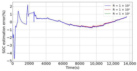
Figure 9.
Measuring the effect of noise covariance on filtering.
It can be seen that the measurement covariance has little effect on the system within a certain range, which proves that the filtering has good robustness. In the experiment, , , is chosen to consider the uncertainty of the system.
The system framework designed in this paper is shown in Figure 10 below: it is divided into online and offline phases. The collected battery data is first trained in the offline phase using the established LSTM + attention network. Then, the Kalman algorithm is used to perform a real-time online update of the collected results.
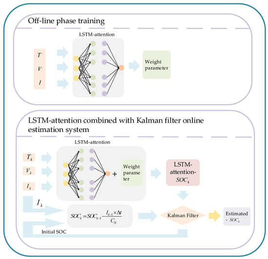
Figure 10.
Overall system structure.
4. Dataset
The EV battery data used in this paper was obtained from the University of Maryland (CALCE) advanced life cycle. The test sample was an 18,650 graphite lithium-electric battery, and the specific specifications of this battery type are shown in Table 1 below.

Table 1.
Lithium battery parameters.
The battery was placed at 0, 25, and 45 °C for charge and discharge experiments, respectively. The discharge includes the US06, DST, FUDS working conditions, which is used to simulate different driving conditions of electric vehicles. Figure 11 below shows the discharge curves for each operating condition in one cycle at 25 degrees Celsius.
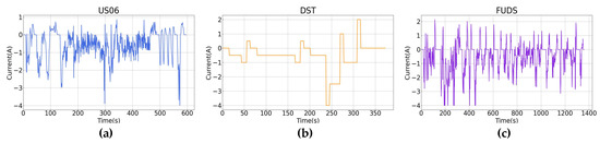
Figure 11.
Discharge current curve for each working condition: (a) US06 condition; (b) DST condition; (c) FUDS condition.
From the above figure, it can be known that there is a significant difference in the variation of current with time for each working condition discharge. US06 is more complicated, while the discharge current of DST working condition is relatively simple.
Figure 12 below shows the curves of current, voltage, and SOC versus time for the entire experimental testing process of the battery under the three conditions of US06, DST, and FUDS. First, the battery is charged with a cross-current charge current of 1 A; when the voltage reaches 4.2 V, the constant voltage discharge starts, keeping the voltage constant. Once the current reaches below 20 mA, the battery is rested; after resting, the battery is discharged with a cross-current discharge current of 1 A, and it has been discharged cross-currently until the working condition is discharged. Two working condition discharge starting capacities are set in the experiment, 50% and 80%, respectively.
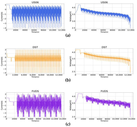
Figure 12.
The 25 degrees Celsius battery charge/discharge curve: (a) US06 condition; (b) DST condition; (c) FUDS condition.
To fully test the robustness of the network, data collected from the US06, DST, and FUDS conditions were used here as the training set; then, the other two conditions were used as the test set, respectively; the input to the network represents the voltage, current, and temperature collected in the time step, with a sampling interval of 1 s, respectively.
The experiments in this article were conducted with an Intel I7 12700KF CPU, RTX3070TI graphics card, and Windows 10 operating system, Tensorflow-keras framework, Python version 3.7, US06, DST, and FUDS conditions, with 200 training epochs and training times of 15, 8, and 20 min, respectively. The training epochs for US06, DST, and FUDS cases were 200, and the training times were 15, 8, and 20 min, respectively. Subsequent Kalman filter processing was performed using MATLAB.
To evaluate the accuracy of the proposed network and curve fit between the predicted and true values, MAE and RMSE are used here as metrics for the evaluation. MAE denotes the mean value of the absolute error, and RMSE denotes the squared open root sign of the difference between the true value and the error, and they can be described by the following equation.
is the predicted value, is the actual value, and is the sample size.
5. Result and Discussion
5.1. SOC Estimation at Room Temperature
In this section, the test results of the proposed network and LSTM network, each combined with Kalman algorithm, are compared. Table 2, below, records the estimation errors for each training test set during the experiments at room temperature.
Table 2.
SOC error at room temperature.
Figure 13 below shows the respective SOC estimation results with SOC error plots at room temperature (25 °C).
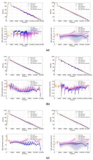
Figure 13.
SOC prediction results at room temperature: (a) US06 condition training, FUDS (left) DST (right) condition test; (b) DST condition training, US06 (left), FUDS (right) condition test; (c) FUDS condition training, US06 (left), DST (right) condition test.
It can be seen that the LSTM–attention algorithm proposed in this paper had smaller error and better curve fitting than LSTM in every condition; after updating LSTM–attention with Kalman, the curve was smoother and error was further reduced. It can be seen that the LSTM–attention–Kalman was more effective than LSTM alone; LSTM–attention or LSTM combined with Kalman, no matter which condition was used as the training set, showed a strong robustness. The maximum RMSE does not exceed 1.9%, and the prediction results do not show much fluctuation, which is more applicable in practical application scenarios.
5.2. SOC Estimation at Different Temperatures
In the actual driving of electric vehicles, extreme weather, such as extreme cold or heat, will be encountered. The internal chemistry of the lithium battery is closely related to the temperature. Figure 14 below shows the SOC error plots of the US06 operating condition test at 0, 25, and 45 °C using the LSTM network when DST did the training set. At low temperature, the error even exceeded 10% at one point, which was due to the fact that the internal chemistry of the battery was not active at low temperature, resulting in difficultly capturing the characteristics. Because of this, the model needs to meet good robustness at different temperatures, in order to meet practical engineering requirements.
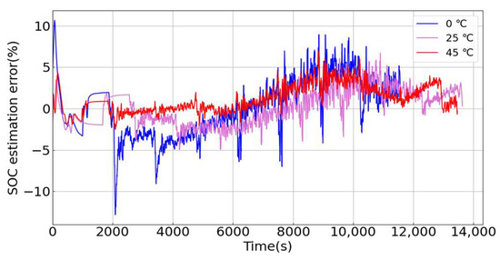
Figure 14.
Effect of temperature on SOC estimation results.
Table 3 shows the SOC estimation errors of the network at 0, 25, and 45 °C, when US06 is the training set and FUDS and DST are the test sets. Experimentally, it can be said that our proposed model achieved an average RMSE of 1.043% at 0 °C, 0.641% at 25 °C, and 0.935% at 45 °C. In contrast, the average RMSE of LSTM were 4.684% at 0 °C, 3.623% at 25 °C, and 3.752% at 45 °C. The average RMSE of LSTM–attention were 2.3% at 0 °C, 1.699% at 25 °C, and 1.72% at 45 °C. It can be seen that the proposed model performed better than the two network models, LSTM and LSTM–attention, on any test set and at any temperature.
Table 3.
US06 does the training set with different temperature SOC errors.
Figure 15 shows the comparison results of each model, when US06 was the training set. It can be seen that the maximum error of the LSTM–attention–Kalman algorithm proposed in this paper did not exceed 5% under each temperature test in each working condition, while the maximum error of the common LSTM network test even exceeded 15%, which shows that the algorithm proposed in this paper has strong stability in each temperature test. The error of the algorithm in this paper basically fluctuated around 2%, while the LSTM or LSTM–attention algorithm basically fluctuated at 10%. This shows that the algorithm proposed in this paper also has strong robustness.
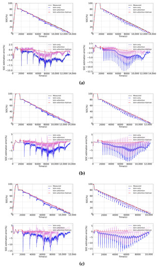
Figure 15.
Effect of each temperature on SOC estimation results when US06 does the training set: (a) 45 °C, FUDS (left) DST (right) service test; (b) 25 °C, FUDS (left) DST (right); (c) 0 °C, FUDS (left) DST (right).
Table 4 shows the SOC estimation errors of the network at 0, 25, and 45 °C, when DST is used as the training set and US06 and FUDS are used as the test sets. Since the DST data has the simplest transformation during the working discharge, it does not have strong robustness when doing the training set, and the other two working conditions are relatively complex, in terms of discharge current and voltage transformation. Under LSTM–attention–Kalman, the average RMSE reaches 1.83% at different temperatures and operating conditions, while the LSTM and LSTM–attention are 2.68% and 2.16%. Experiments show that the model in this paper also performs significantly better than ordinary neural networks in DST training.
Table 4.
DST does the training set with different temperature SOC errors.
Figure 16 shows the comparison results of each model.
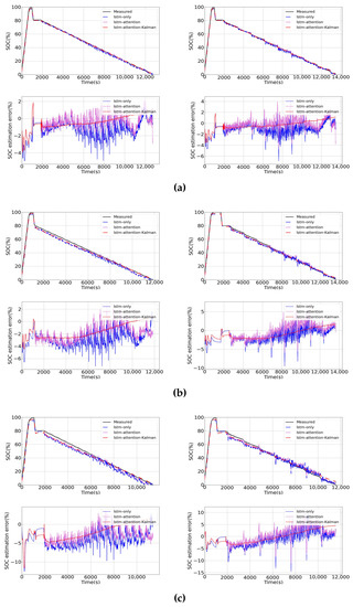
Figure 16.
Effect of each temperature on SOC estimation results when DST does the training set: (a) 45 °C, US06 (left), FUDS (right) service test; (b) 25 °C, US06 (left), FUDS (right); (c) 0 °C, US06 (left), FUDS (right).
Similarly, FUDS was used as the training set and US06 with DST was used as the test set. Table 5 gives the SOC errors at different temperatures for the other two operating conditions when FUDS was trained.
Table 5.
FUDS does the training set with different temperature SOC errors.
Figure 17 shows the comparison of the results of different models at different temperatures. Under LSTM–attention–Kalman, the average RMSE reached 0.86% at different temperatures and operating conditions, while the LSTM and LSTM–attention were 1.83% and 1.52%.
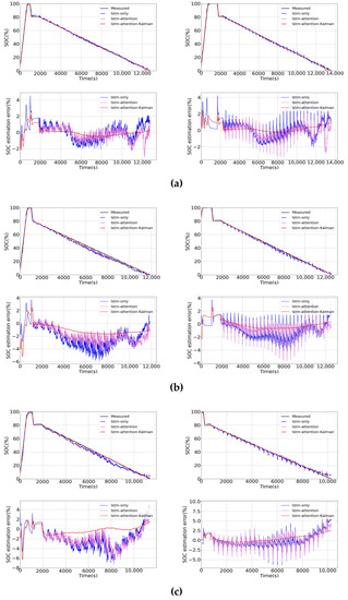
Figure 17.
Effect of each temperature on SOC estimation results when FUDS does the training set: (a) 45 °C, US06 (left), DST (right) service test; (b) 25 °C, US06 (left), DST (right); (c) 0 °C, US06 (left), DST (right).
5.3. SOC Estimation at Different Initial Power Levels
In practical applications, it is not possible to obtain the initial SOC value accurately every time. In addition, if the battery management system is restarted, due to some faults, the initial SOC value may be lost, which requires the model to have good robustness at different initial power levels. Therefore, the initial power levels were set to 80%, 60%, and 50%, and the experiments were conducted separately. The results are shown in Figure 18.
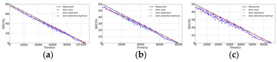
Figure 18.
SOC estimation at different power levels: (a) 80%; (b) 60%; (c) 50%.
Through these experiments, we can see that the SOC value converged correctly to the true value, regardless of the initial value, with a maximum error of no more than 5%, which meets the needs of practical engineering.
5.4. Summary of Comparison with the Latest Methods
The algorithm LSTM–attention–Kalman proposed in this paper is compared with the existing state-of-the-art algorithms LSTM [31], as well as LSTM–Kalman [34], which are summarized in Table 6.
Table 6.
Comparison and summary with existing methods.
6. Conclusions
In this paper, an algorithm combining LSTM–attention and Kalman filtering is proposed to estimate the battery SOC in dynamic systems. The method first uses the measured temperature, voltage, and current data for processing and passes them into an LSTM–attention network to obtain an approximate SOC value. It then uses Kalman’s algorithm to further improve the reliability of the algorithm. It is demonstrated that the proposed method can learn the internal dynamics of the battery well and has higher estimation accuracy than both the simple LSTM–attention and LSTM–Kalman under different temperatures, working conditions, and initial charge conditions, with DST for training at room temperature and two other working conditions for testing. The average RMSE of LSTM–attention-Kalman was 0.466 and 0.3995 percentage points higher than that of LSTM–attention and LSTM–Kalman, respectively. In addition, the method is data-driven and does not require circuit models, very precise tuning of network parameters, or the construction of OCV–SOC lookup tables.
With the high-speed development of the GPU and wide application of the BMS system, it provides a lot of technical, as well as data, support for the training of neural network. The use of collected big data for SOC estimation has very broad prospects. Therefore, in the future, the machine learning method will become a powerful tool for lithium battery SOC estimation.
Author Contributions
Conceptualization, X.Z. and Y.H.; methodology, X.Z.; software, Z.Z.; validation, H.L. and Z.Z.; formal analysis, Y.Z.; investigation, Y.Z.; resources, M.G.; data curation, M.G.; writing—original draft preparation, X.Z.; writing—review and editing, X.Z.; visualization, Z.Z.; supervision, M.G.; project administration, H.L.; funding acquisition, H.L. All authors have read and agreed to the published version of the manuscript.
Funding
This work was supported by National Key Research and Development Program of China (2020YFB1710600), Fundamental Research Funds for the Provincial Universities of Zhejiang (GK229909299001-404), and Key Research and Development Program of Zhejiang Province (2021C01111).
Institutional Review Board Statement
Not applicable.
Informed Consent Statement
Not applicable.
Data Availability Statement
Research Data at CALCE Battery Group (umd.edu), URL: https://web.calce.umd.edu/batteries/data.htm#INR18650.
Conflicts of Interest
The authors declare no conflict of interest.
References
- Shen, H.; Zhou, X.; Wang, Z.; Wang, J. State of charge estimation for lithium-ion battery using Transformer with immersion and invariance adaptive observer. J. Energy Storage 2021, 45, 103768. [Google Scholar] [CrossRef]
- Rahman, A.; Lin, X.; Wang, C. Li-Ion Battery Anode State of Charge Estimation and Degradation Monitoring Using Battery Casing via Unknown Input Observer. Energies 2022, 15, 5662. [Google Scholar] [CrossRef]
- Bao, Y.; Chang, F.; Shi, J.; Yin, P.; Zhang, W.; Gao, D.W. An Approach for Pricing of Charging Service Fees in an Electric Vehicle Public Charging Station Based on Prospect Theory. Energies 2022, 15, 5308. [Google Scholar] [CrossRef]
- Tian, Y.; Lai, R.; Li, X.; Xiang, L. A combined method for state-of-charge estimation for lithium-ion batteries using a long short-term memory network and an adaptive cubature Kalman filter. Appl. Energy 2020, 265, 114789. [Google Scholar] [CrossRef]
- Rahman, A.; Lin, X. Li-ion battery individual electrode state of charge and degradation monitoring using battery casing through auto curve matching for standard CCCV charging profile. Appl. Energy 2022, 321, 119367. [Google Scholar] [CrossRef]
- Xia, B.; Zhang, G.; Chen, H.; Li, Y.; Yu, Z.; Chen, Y. Verification Platform of SOC Estimation Algorithm for Lithium-Ion Batteries of Electric Vehicles. Energies 2022, 15, 3221. [Google Scholar] [CrossRef]
- Yang, B.; Wang, Y.; Zhan, Y. Lithium Battery State-of-Charge Estimation Based on a Bayesian Optimization Bidirectional Long Short-Term Memory Neural Network. Energies 2022, 15, 4670. [Google Scholar] [CrossRef]
- Zhang, S.; Wan, Y.; Ding, J.; Da, Y. State of Charge (SOC) Estimation Based on Extended Exponential Weighted Moving Average H∞ Filtering. Energies 2021, 14, 1655. [Google Scholar] [CrossRef]
- Yang, K.; Tang, Y.; Zhang, Z. Parameter Identification and State-of-Charge Estimation for Lithium-Ion Batteries Using Separated Time Scales and Extended Kalman Filter. Energies 2021, 14, 1054. [Google Scholar] [CrossRef]
- Snihir, I.; Rey, W.; Verbitskiy, E.; Belfadhel-Ayeb, A.; Notten, P.H.L. Battery open-circuit voltage estimation by a method of statistical analysis. J. Power Sources 2005, 159, 1484–1487. [Google Scholar] [CrossRef]
- Rezaei, O.; Habibifar, R.; Wang, Z. A Robust Kalman Filter-Based Approach for SoC Estimation of Lithium-Ion Batteries in Smart Homes. Energies 2022, 15, 3768. [Google Scholar] [CrossRef]
- Pei, L.; Lu, R.; Zhu, C. Relaxation model of the open-circuit voltage for state-of-charge estimation in lithium-ion batteries. IET Electr. Syst. Transp. 2013, 3, 112–117. [Google Scholar] [CrossRef]
- Rahimi-Eichi, H.; Ojha, U.; Baronti, F.; Chow, M.U. Battery Management System: An Overview of its Application in the Smart Grid and Electric Vehicles. IEEE Ind. Electron. 2013, 7, 4–16. [Google Scholar] [CrossRef]
- Chen, J.; Ouyang, Q.; Xu, C.; Su, H. Neural Network-Based State of Charge Observer Design for Lithium-Ion Batteries. IEEE Trans. Contr. Syst. Technol. 2017, 26, 313–320. [Google Scholar] [CrossRef]
- He, H.; Xiong, R.; Fan, J. Evaluation of Lithium-Ion Battery Equivalent Circuit Models for State of Charge Estimation by an Experimental Approach. Energies 2011, 4, 582–598. [Google Scholar] [CrossRef]
- Nguyen, T.; Khan, A.; Ko, Y.; Choi, W. An Accurate State of Charge Estimation Method for Lithium Iron Phosphate Battery Using a Combination of an Unscented Kalman Filter and a Particle Filter. Energies 2020, 13, 4536. [Google Scholar] [CrossRef]
- Sun, F.; Hu, X.; Zou, Y.; Li, S. Adaptive unscented Kalman filtering for state of charge estimation of a lithium-ion battery for electric vehicles. Energy 2011, 36, 3531–3540. [Google Scholar] [CrossRef]
- Zhang, F.; Liu, G.; Fang, L.; Wang, H. Estimation of Battery State of Charge With H∞ Observer: Applied to a Robot for Inspecting Power Transmission Lines. IEEE Trans. Ind. Electron. 2011, 59, 1086–1095. [Google Scholar] [CrossRef]
- Dong, Z.; Lai, C.S.; Zhang, Z.; Qi, D.; Gao, M.; Duan, S. Neuromorphic extreme learning machines with bimodal memristive synapses. Neurocomputing 2021, 453, 38–49. [Google Scholar] [CrossRef]
- Cortes, C.; Vapnik, V. Support-Vector Networks. Mach. Learn 1995, 20, 273–297. [Google Scholar] [CrossRef]
- Li, R.; Xu, S.; Li, S.; Zhou, Y.; Zhou, K.; Liu, X.; Yao, J. State of Charge Prediction Algorithm of Lithium-Ion Battery Based on PSO-SVR Cross Validation. IEEE Access 2020, 8, 10234–10242. [Google Scholar] [CrossRef]
- Huang, G.; Zhu, Q.; Siew, C. Extreme learning machine: Theory and applications. Neurocomputing 2005, 70, 489–501. [Google Scholar] [CrossRef]
- Du, J.; Liu, Z.; Wang, Y. State of charge estimation for Li-ion battery based on model from extreme learning machine. Control. Eng. Pract. 2014, 26, 11–19. [Google Scholar] [CrossRef]
- Dong, Z.; Lai, C.S.; Qi, D.; Xu, Z.; Li, C.; Duan, S. A general memristor-based pulse coupled neural network with variable linking coefficient for multi-focus image fusion. Neurocomputing 2018, 308, 172–183. [Google Scholar] [CrossRef]
- Dong, Z.; Lai, C.S.; He, Y.; Qi, D.; Duan, S. Hybrid dual-complementary metal–oxide– semiconductor/memristor synapse-based neural network with its applications in image super-resolution. IET Circuits Devices Syst. 2018, 13, 1241–1248. [Google Scholar] [CrossRef]
- Xia, B.; Cui, D.; Sun, Z.; Lao, Z.; Zhang, R.; Wang, W.; Sun, W.; Lai, Y.; Wang, M. State of charge estimation of lithium-ion batteries using optimized Levenberg-Marquardt wavelet neural network. Energy 2018, 153, 694–705. [Google Scholar] [CrossRef]
- Hannan, M.A.; Hoque, M.M.; Hussain, A.; Yusof, Y.; Ker, P.J. State-of-the-Art and Energy Management System of Lithium-Ion Batteries in Electric Vehicle Applications:Issues and Recommendations. IEEE Access 2018, 6, 19362–19378. [Google Scholar] [CrossRef]
- Chaoui, H.; Ibe-Ekeocha, C.C. State of Charge and State of Health Estimation for Lithium Batteries Using Recurrent Neural Networks. IEEE Trans. Veh. Technol. 2017, 66, 8773–8783. [Google Scholar] [CrossRef]
- Hochreiter, S.; Schmidhuber, J. Long short-term memory. Neural Comput. 1997, 9, 1735–1780. [Google Scholar] [CrossRef]
- Dong, Z.; Ji, X.; Lai, C.; Qi, D.; Zhou, G.; Lai, L. Memristor-Based Hierarchical Attention Network for Multimodal Affective Computing in Mental Health Monitoring. IEEE Consum. Electron. Mag. 2022. [Google Scholar] [CrossRef]
- Yang, F.; Song, X.; Xu, F.; Tsui, K.L. State-of-Charge Estimation of Lithium-Ion Batteries via Long Short-Term Memory Network. IEEE Access 2019, 7, 53792–53799. [Google Scholar] [CrossRef]
- Jiao, M.; Wang, D.; Qiu, J. A GRU-RNN based momentum optimized algorithm for SOC estimation. J. Power Sources 2020, 459, 228051. [Google Scholar] [CrossRef]
- Yang, F.; Zhang, S.; Li, W.; Miao, Q. State-of-charge estimation of lithium-ion batteries using LSTM and UKF. Energy 2020, 201, 117664. [Google Scholar] [CrossRef]
- Yang, Y.; Dong, A.; Li, Y. Temperature Dependent State of Charge Estimation of Lithium-ion Batteries Using Long Short-Term Memory Network and Kalman Filter. In Proceedings of the IECON 2019-45th Annual Conference of the IEEE Industrial Electronics Society 2019, Lisbon, Portugal, 14–17 October 2019; pp. 4335–4340. [Google Scholar]


Publisher’s Note: MDPI stays neutral with regard to jurisdictional claims in published maps and institutional affiliations. |
© 2022 by the authors. Licensee MDPI, Basel, Switzerland. This article is an open access article distributed under the terms and conditions of the Creative Commons Attribution (CC BY) license (https://creativecommons.org/licenses/by/4.0/).