Article

Re-Defining System LCOE: Costs and Values of Power Sources

1
College of Asia Pacific Studies, Ritsumeikan Asia Pacific University, Oita 874-8577, Japan
2
The Institute of Energy Economics, Tokyo 104-0054, Japan
Energies 2022, 15(18), 6845; https://doi.org/10.3390/en15186845
Submission received: 24 August 2022 / Revised: 13 September 2022 / Accepted: 15 September 2022 / Published: 19 September 2022

Abstract

:
The mass introduction of variable renewable energies, including wind and solar photovoltaic, leads to additional costs caused by the intermittency. Many recent studies have addressed these “integration costs,” and proposed novel metrics that replace the traditional metric known as the levelized cost of electricity (LCOE). However, the policy relevance of those metrics remains unclear. In this study, the author investigates and re-defines the concept of system LCOE, referring to prior studies, and proposes concrete methods to estimate them. Average system LCOE allocates the integration cost to each power source, dividing that by the adjusted power output. Marginal system LCOE revises the concept of system LCOE and value-adjusted LCOE proposed by prior studies, to be clearer and more policy-relevant. These metrics are also applied to Japan’s power sector in 2050, suggesting the necessity of aiming for a “well-balanced energy mix” in future power systems with decarbonised power sources.

1. Introduction

1.1. Mass Introdcution of Variable Renewable Energies and Associated Challenges

With the increasing influence of anthropogenic greenhouse gas (GHG) emissions on global climate change, the urgent necessity of reducing them has also become indisputable in recent years. According to a report published by the Intergovernmental Panel on Climate Change (2018) [1], limiting global warming above pre-industrial levels to 1.5 °C with no or limited overshoot, and to below 2 °C, would require global carbon dioxide (CO2) emissions to reach net zero levels by around 2050 and 2075, respectively. As the currently pledged national plans for GHG emission reductions, called Nationally Determined Contributions, are not sufficient to meet these reduction targets [2], stringent efforts for mitigating climate change would be essential in the long term. Under such circumstances, the introduction of variable renewable energies (VRE), such as wind and solar power, is experiencing rapid progression, which has also boosted future targets for VRE expansion [3].
After the Russian invasion of Ukraine in February 2022, the situation regarding energy systems changed drastically. Soaring energy prices reminded people once again of the importance of a stable supply of fossil fuels and energy security. However, even in the midst of this energy crisis, movements towards addressing climate change never stopped. Rather, European nations are struggling to shift away from fossil fuels in the long run, which would lead to a massive introduction of alternative energies. From this perspective, we could expect a rapid progression of the diffusion of renewable energies, even after the current chaotic situation.
The challenges facing a high penetration of VRE are usually proposed with reference to the “integration cost.” This should include, at least conceptually, all the costs and benefits related to the large-scale introduction of VRE, such as the costs of environmental and ecological destruction by the massive construction of windmills and solar farms, and the benefits for energy security with reduced use of fossil fuels. Although there are continuous efforts to estimate the “full cost of electricity provision” in this sense [4], it is usually difficult to monetize all the costs and benefits, and even when it is possible, the estimated costs bear significant uncertainties. Nonetheless, as assessing only the costs that can be estimated clearly in monetized terms is still useful and policy-relevant, many studies address this important issue.
Although there have been many studies addressing this issue, as shown later, most of them calculate the integration costs for the power system with high or low VRE penetration, but not for each technology. However, policymaking does require the estimation of power generation cost by technology. Traditionally, the economics of the power sector have been assessed using a metric known as the levelized cost of electricity (LCOE) [5], which represents unit power generation cost by technology. It calculates the net present value of all the lifecycle costs related to a certain technology, from plant construction to decommissioning and waste disposal, as a cost per unit of power generation. LCOE has proven to be a powerful metric with strong and consistent theoretical backgrounds [6], although several studies have been attempted to modify it in accordance with real energy markets [7,8]. One could understand this as a linear approximation of the changes in the total cost of the power system caused by the substitution of power sources. Note that because of this linearity, traditional LCOE can be regarded as representing both the “marginal” and the “average” cost of a specific technology at the same time.
In contrast, the integration cost described above usually refers to the nonlinear relationship between the penetration of VRE and the total system cost. The required volume of power storage systems, for example, does not increase proportionally to VRE penetration; while it is almost negligible with low penetration levels, it increases nonlinearly with increasing demand for balancing the intermittency of VRE. Although the cost structure of storage systems can be assessed with a similar metric known, such as the levelized cost of storage (LCOS) [9] or annualized life cycle cost of storage (LCCOS) [10], it cannot capture the nonlinearity related to the substitution of power sources under a high penetration of VRE. This suggests that the economic analyses of future power systems would require novel metrics that represent the nonlinear nature of the integration cost, which remains beyond the scope of traditional analyses using LCOE or LCOS.
Investigating the nonlinear nature of power generation should also be useful from the perspective of energy system modeling. For example, calculations using large-scale mathematical models, such as integrated assessment models (IAM), usually do not incorporate detailed representations of the power sector; however, they do employ some simplification. Some studies exploit a method that uses residual load duration curves (RLDCs) to calculate integration cost [11,12]. As this method estimates a part of the profile costs with high penetration of VRE, other integration costs, such as balancing costs, grid costs, and storage costs, cannot be estimated simply, although it may be possible to consider some of these cost components by linking the model with another one [13]. Given that the changes in the economics of the power sector caused by VRE can exert significant influence on the estimation of future GHG reduction targets of a country, or of the whole world, it should be of great importance to establish new metrics “beyond LCOE,” to provide a simple representation of the nonlinear changes in the power sector.
In view of these situations, several new metrics have been proposed in the literature, such as value-adjusted LCOE (VALCOE) by the International Energy Agency (IEA) [14,15] and system LCOE by Hirth et al. (2016) [16], as shown later, although we should note that they do not always have very clear definitions [17], and the relationships between them can be ambiguous. Referring to these prior works, in the previous work [18], the author attempted to propose two metrics named relative marginal system LCOE and average system LCOE, to address these questions. However, the previous work had the following unsolved issues: First, the metrics proposed were not presented with exact mathematical formulations. For example, relative marginal system LCOE presented in the study may not be defined uniquely, at least as it is. Moreover, although the metrics were defined as a function of variables representing power generation of each technology, we could argue that they should also be dependent on other factors, such as the type of policies to achieve high shares of VRE, because electricity prices, or “values” of power generation, should be dependent on the type of policies, and the “values” in turn should affect the economic feasibility of power generating technologies. These issues were not addressed in the previous paper. Second, while we can compare the relative costs of different technologies in one region using relative marginal system LCOE, this metric cannot present a comparison between the costs of power generating technologies in different regions. To do this, we would need another metric that is designed more elaborately. Third, the previous paper tried to show that with high shares of VRE, their relative marginal system LCOE soar, which leads to deteriorating cost competitiveness. However, as actual policies in many countries aim to mitigate the negative impacts of high VRE shares by enhancing the flexibility of power demand, using such advanced technologies as vehicle to grid (VtoG), simple calculation of the metrics may not contribute to realistic policy making. Fourth, although relative marginal system LCOE presented in the paper was a metric quite similar to system LCOE presented by Hirth et al. (2016) [16], the difference between the two metrics has never been discussed in detail.
Under these circumstances, in this article, the author identified the following research questions: Considering all the situations, how should metrics “beyond LCOE” designed? How should they be applied to real energy systems, and what policy recommendations do they imply? As answering these questions is important from policy perspectives, as well as from an academic viewpoint, the author has been engaged in studies in this field, and accordingly refined the analysis in this article. Specifically, he revisited the concepts of the metrics with full mathematical formulations and presented a discussion proposing another metric called marginal system LCOE. He then illustrated these concepts and methods using a simple linear programming (LP) model assuming two power generating technologies, also applying them to a real system, namely Japan’s decarbonized power sector in 2050, following previous works [19,20].
The study was conducted with the following research hypotheses: First, although the various metrices presented in past studies are policy relevant to a certain extent, there is supposed to be some confusion and misunderstanding. Thus, elucidating the mathematical background and formulation should contribute greatly to academic and practical values. Second, specific policy measures to enhance demand flexibilities are supposed to mitigate cost hikes associated with a high penetration of VRE. Through quantitative analyses, we should be able to measure the usefulness of those measures.
The relevance of system LCOE in actual policymaking is obvious. For example, the Japanese government revises its estimation of LCOE of various technologies once in nearly five years. In the latest publication [21], it presented the results of tentative calculation of relative marginal system LCOE for five technologies (coal, natural gas, nuclear, solar PV, and onshore wind) for the year 2030, referring to the author’s previous work [18]. Moreover, the Japanese government has been engaged in the assessment of decarbonization pathways through quantitative analyses using mathematical models that take into account those metrics, as well as traditional LCOE and integration costs. Likewise, the UK government presented “enhanced levelized costs” for five technologies (natural gas, natural gas with CCS, solar PV, onshore wind, and offshore wind), resembling relative marginal system LCOE [22]. As such, the estimation of marginal costs of power generation has been regarded as useful for policymaking, complementing the conventional notion of LCOE.
The contribution of this work to the literature is three-fold. First, to the best of the author’s knowledge, this is the first study to describe clearly a method to allocate the integration cost to each power generating technology, and then estimate the average system LCOE by technology consistently. As average costs and marginal costs can exhibit very different pictures, estimating both costs should be important from policy perspectives. To be more specific, estimation of marginal system LCOE would suggest realistic challenges associated with achieving high shares of VRE, while average system LCOE would imply that strong measures to promote the diffusion of VRE may not lead to very large economic damages. Second, this study proposes a consistent method to estimate marginal system LCOE by technology. Although both system LCOE_HUE and VALCOE can be viewed as indicating the marginal cost of a technology, the metrics presented in this study are defined more consistently, for example, in that with those we can compare the costs of different technologies in different regions and provide broader information considering both “marginal” and “average” costs. Third, this work applies these metrics to real systems to draw policy implications, and to give insights related to a simple representation of the power sector, that can also be applied for use in IAM.
The remainder of this article is organized as follows: The following subsections are a literature review. Section 2 overviews the proposed concepts, such as average system LCOE and the allocation of the integration cost, relative marginal system LCOE, and marginal system LCOE, and addresses the issues raised above, with exact definitions and detailed discussion being found in Appendix B and Appendix C. The section also describes the methods to conduct the calculation. Section 3 provides numerical calculation results and discussions. Finally, Section 4 proposes conclusions and policy implications.

1.2. Literature Review: High Penetration of VRE and Integration Cost

The estimation of integration costs with high shares of VRE has long been recognized as an important research topic with high policy relevance, with many studies published after 2010. In many cases, integration costs are classified into three categories: balancing costs, grid costs, and profile costs [4,23]. As it is usually difficult to encompass all these costs with one mathematical model, many studies have investigated a part of these costs for specific regions. Although earlier studies focused on cost increases with relatively lower shares of VRE, after 2017, we find many studies that estimate the costs of achieving very high shares over 50%, for many countries and regions of the world. While most studies are by western researchers focusing on western countries, e.g., the United States [24,25] and Europe [26,27], among many, some research groups [28,29] have continuously been publishing related studies explicitly targeting almost all countries. Apart from them, detailed analyses are also published with a special focus on non-Western counties, such as China [30], India [31], and Japan [19,32].
Some studies have also tried to review the results of these prior studies. Hirth et al. (2015) [33] concluded that with high VRE shares, profile costs become larger than balancing costs, and amount to 2.5–3.5 eurocents/kWh with 40% penetration. Heptonstall et al. (2017) [34] also reviewed related studies to conclude that the cost increases are 0.5–2 pence/kWh for 30% and can rise to around 4 pence/kWh for 50%. According to the Organization for Economic Co-operation and Development (OECD)/Nuclear Energy Agency (NEA) (2018) [4], the cost rise is 2–4 U.S. cent/kWh for 30%. However, these numbers are subject to large uncertainties. For example, while an older study by the same organization [35] estimates the integration cost at 3–8 U.S. cent/kWh for 30% penetration of solar photovoltaic (PV), another study by OECD/NEA (2019) [36] proposes an integration cost of around 2 U.S. cent/kWh for the same share of VRE, although the latter study is not a literature review but is based on original model calculations. At least part of this uncertainty may result from the inappropriateness of the methodologies, as highlighted by Heard et al. (2017) [37], to which rebuttals are also published [38,39], forming ongoing discussions.

1.3. Literature Review: Costs/Values of Power Sources and Proposed Metrics “beyond LCOE”

As stated in Section 1, designing good metrics to represent integration costs by technology is another challenge. To this end, several metrics, including system LCOE by Hirth et al. (2016) [16], which is referred to as system LCOE_HUE throughout this article, VALCOE by the IEA [14], levelized avoided cost of electricity (LACE) by U.S. Department of Energy (DOE) [40,41], and levelized full system costs of electricity (LFSCOE) by Idel (2022) [42], have been proposed to represent power generation cost by technology under high penetration of VRE. Most of these new metrics feature the estimation of the “values,” as well as the costs, of power sources. For example, system LCOE_HUE extends the notion of traditional LCOE by adjusting it with deviation in values. VALCOE by the IEA also applies similar adjustments, focusing on practical applications using market prices observed in the real world. U.S. DOE refers more directly to the unit value as the levelized avoided cost of electricity (LACE), comparing LCOE and LACE to estimate the cost competitiveness of technologies. As suggested by this terminology, the cost and the value are both sides of one coin; in this subsection, the author overviews how the cost, the value, and the proposed new metrics are mutually related. Among these metrics, LFSCOE by Idel (2022) [42] is different from other metrics in that it calculates the cost of VRE when the market is occupied only by one power generating technology. For this reason, this metric is not discussed much in this article, which aims to capture the economics of real power systems.
When VRE is massively introduced to a system, the wholesale electricity prices decline significantly by a well-known “merit-order effect,” caused by the very small operating cost of VRE. This effect has been analyzed extensively, focusing mainly on western countries, which are experiencing rapid advances in VRE introduction [43,44,45,46]. However, other studies propose similar analyses for Asian countries [47,48,49]. Several studies published in the first half of the 2010s advocated that this effect can bring large benefits to consumers [50], while more recent studies tend to regard this effect as an important challenge for the future deployment of VRE, in which respect it is called the “cannibalization” effect [51,52], with the “market values”, or the rewards to power generating facilities, declining considerably along with the deployment of the same kind of power generating technology. Green and Léautier (2015) [53] analyzed this effect for wind power in the United Kingdom, to conclude that subsidies to VRE may never end even if its costs continue to decline rapidly in the future.
In the context of economic analysis of power systems, we can think of “values of supplies” and “values of demands.” The value Vi of a power supply technology i is defined as the total annual revenue from power markets, such as the wholesale electricity market and the capacity market. The value of demand VL is calculated as the total amount of money to be paid to the market to satisfy the demand. This article uses lower-case letters to denote unit costs and values, namely the costs/values divided by the power output; vi, the unit value of technology i, is defined as the value Vi divided by the power output xi, and the unit value of demand vL is the value of demand VL divided by the total annual electricity demand E. Similarly, annualized costs and unit costs are denoted as C* and c*, respectively. The unit cost ci is identical to the LCOE of technology i, which reflects the load factor of the technology in the given energy mix. Note that in the linear programming framework that is exploited to illustrate the metrics in this article, Ci and Vi are defined as the part of the objective function C, that explicitly relates to technology i, and the sum of all the shadow prices that relate to i, with regard to the constraints in the linear modeling problem (see Appendix A). We should also note that the metrics presented in this study are defined not only in a linear programing model, but in more general terms.
System LCOE_HUE is defined as follows [16]:
L H U E   i = c i v i + v L
System LCOE_HUE of technology (or “source”) i is defined as its LCOE, calculated with the load factor in the energy mix (or the “state”), minus the unit value of i, plus the unit value of demand. If technology i is not “constrained”, i.e., the annual power output of i is not fixed, then the unit value vi equals the LCOE ci, and the system LCOE_HUE of i is identical to the value of demand vL. In case all the technologies are unconstrained, the system LCOE_HUE of all of them take the same value vL at the optimal point. As is shown in Appendix A, system LCOE_HUE, as well as VALCOE which the author argues is a metric essentially identical to system LCOE_HUE, measures the difference from the optimal point with respect to each technology. This also holds true for relative marginal system LCOE, of which the previous study (2021) [18] proposed a preliminary investigation, and enhanced levelized cost by BEIS (2020) [22], which has been calculated with the dispatch model owned by the UK government, although not all the detailed assumptions have been disclosed. While these are attempts to combine the cost and the value into one metric, other attempts do not combine, but compare the cost and the value to assess cost competitiveness. Levelized avoided cost of electricity (LACE) by the U.S. EIA [40] is essentially identical to the unit value vi. If the deployment of technology i is smaller than the optimal level, the value vi exceeds the cost ci, and additional deployment of i is profitable.
Note that the relationship between the concept of “integration cost” and these metrics is not straightforward. For example, with high penetration of VRE, the load factors of the conventional facilities in the system decline, leading to considerable cost increases. This type of additional cost is usually regarded as part of the “profile cost,” which is in turn a part of the integration cost [23]. However, when the IEA adjusts the LCOE of a power source to calculate the VALCOE, the LCOE already includes the cost increase caused by the decline in the load factor. Thus, although the “value adjustment” by the IEA should be closely related to the concept of the integration cost, as VALCOE has been intended to capture the non-linear nature of it, they do not refer to the same thing.
Another ambiguity is related to the distinction between the average cost and the marginal cost. As described above, LCOE represents both of them at the same time, only because it assumes linearity. Then, what about system LCOE_HUE and VALCOE, which attempt to capture non-linearity? Obviously, we need to reinvestigate these concepts to obtain a clearer understanding of the nature of the problem, which has not been undertaken in the literature.

2. Theoretical Background and Methodology

This study adopted the following methodology: First, the author described a mathematical framework of the metrics “beyond LCOE,” taking into account the findings of past studies. Although this is a purely theoretical work, it is an important part of the whole study, as described in Section 2.1 and Section 2.2, as well as in Appendix B and Appendix C. Then, quantitative modeling analyses were conducted, using an optimization model exploiting the LP method, following the methodology adopted in prior studies. The methods are described more in depth in Section 2.3.

2.1. Metrics Proposed in the Previous Study

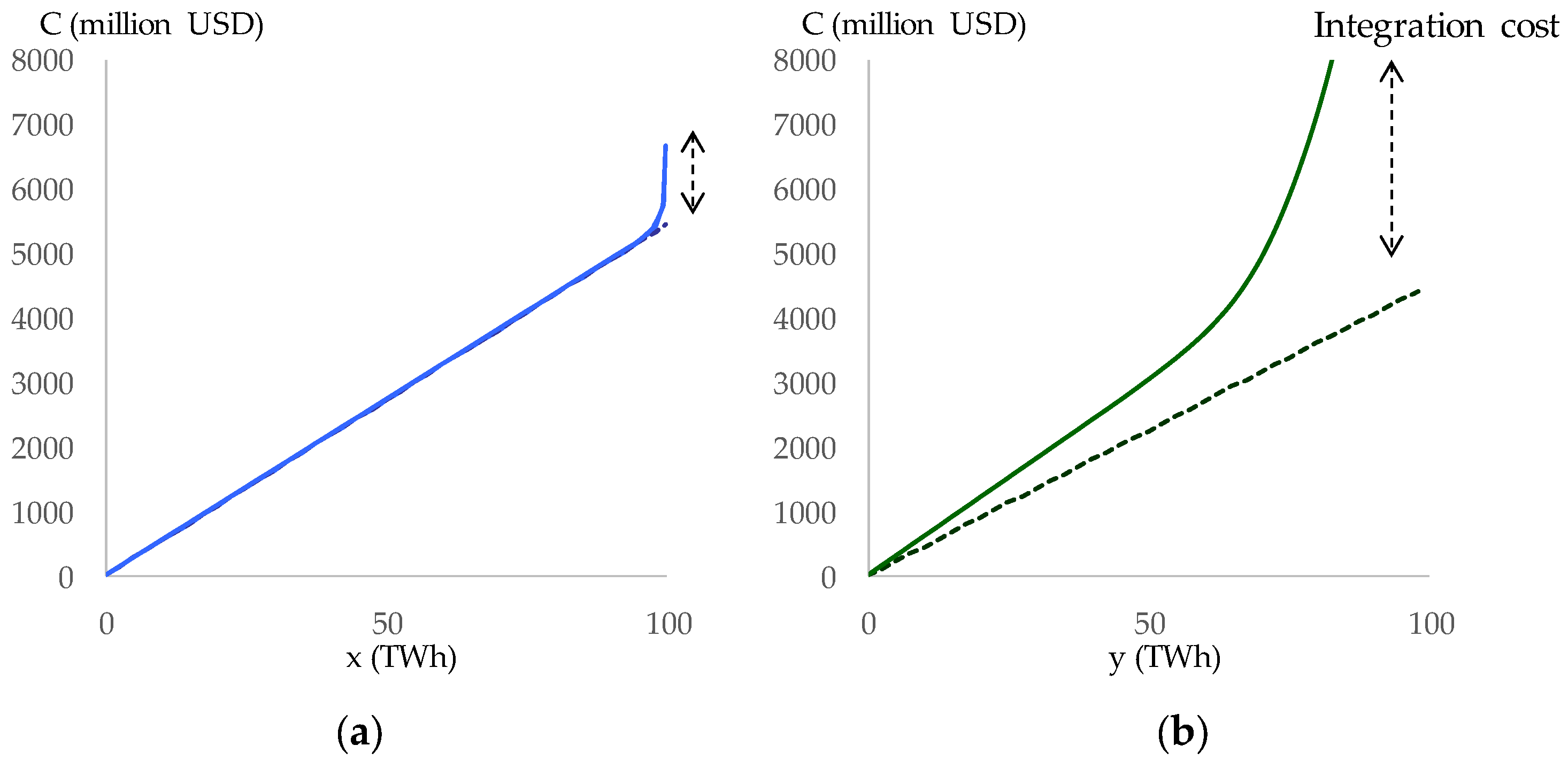
This section proposes the concepts of system LCOE, with reference to past studies. Figure 1 illustrates the concept of integration cost for a simple system with two technologies, that is, a conventional (thermal) power generation technology and a VRE. The LCOE, denoted as Lconv and LVRE, respectively, of the two technologies, are defined as those calculated with the maximum possible load factors (for example, 80% for the conventional technology and 22% for VRE in the example shown in Appendix D). The integration cost I is defined as the gap between the total annual cost C and the sum of Cconv and CVRE, which are the annual power outputs multiplied by the LCOE.
In the prior study [18], the author proposed the concepts of relative marginal system LCOE and average system LCOE. They are roughly described as follows, using the total cost C and the integration cost I for calculation.

2.1.1. Relative Marginal System LCOE

Relative marginal system LCOE refers to the marginal change in the total cost C, associated with the substitution of two types of power generation. In the case of the system with two technologies illustrated by Figure 1, the slope of the total cost C = Cconv + CVRE + I represents the difference in the marginal cost of the conventional technology and that of VRE; if the former is larger, the slope is negative. Note that only the difference in the marginal costs of the two technologies can be measured as the derivative of C.
More generally, suppose that in a power system, in which the annual power output of technology i is denoted as xi, we increase xi marginally by dxi. This must be complemented by decreases in outputs of other technologies. Here, we assume that it is complemented by a decrease in x0, which is the annual output of a “reference” technology. For example, suppose that technology i denotes solar PV, while coal-fired power generation is selected as the reference technology 0. Then, R i d x i = d x 0 may hold with 0 < Ri < 1, and Ri may be considerably smaller than 1, because of electricity losses related to power storage or transmission. Mathematically, Ri can be calculated by R i = 1 T / x i , with T being the electricity losses caused by changes in the power generation mix.
Relative marginal system LCOE LRi of technology i is defined by the following equation:
L R i = 1 R i C x i C x 0 + L R 0
Equation (2) implies that with a marginal substitution between xi and x0, d C = L R i L R 0 d x 0 . That is, the difference between the relative marginal system LCOE of i and 0 indicates the marginal increase in C caused by the substitution between the outputs of the two technologies by one unit. As the term “relative” implies, only the difference between the relative marginal system LCOE of two technologies is meaningful. In many cases, it would be convenient to define LR0 as equal to a constant value, e.g., the LCOE of the reference technology, and calculate LRi by adding the estimated difference by Equation (2).

2.1.2. Average System LCOE

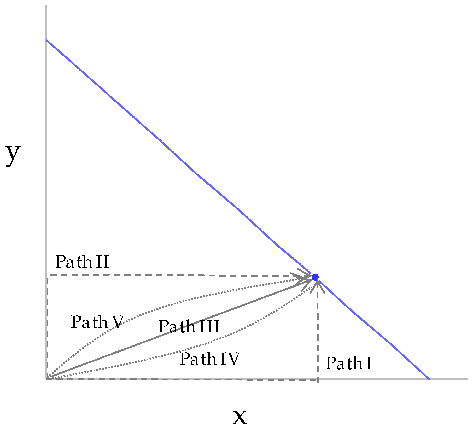
We can also calculate the “average” cost, or the average system LCOE LAi, of power source i by allocating the integration cost I to each technology and dividing it by the power output. This allocation has methodological complexities. In a system with strong non-linearity, the cost changes associated with different technologies vary depending on the order of the introduction of the technologies. If we introduce solar PV to a system only with conventional technologies, and then introduce wind power, the cost increase is larger for wind power than for solar PV, and vice versa. In this regard, the author proposed a method in which all the power outputs are increased equally from the origin of the coordinate, using a straight integration path. Here, the “origin of the coordinate” represents the zero-cost state, in which electricity is supplied with a hypothetical “costless” technology, without any fixed and variable costs and with unlimited flexibility. This method meets several fundamental requirements that such cost allocation policies must satisfy. Note that the integration cost is allocated not only to VRE, but also to conventional technologies. As an example, in a power system only with coal-fired power generation, the load factor is usually lower than the maximum value, for example, 80% to meet the changing electric demand. According to the definition, the cost increase originating from the lower load factors should be viewed as part of the integration cost, caused by the inflexibility of coal-fired power generation.

2.2. Additional Definitions and Discussions over the Metrics

This subsection addresses several issues unresolved in the previous work [18]. They include a comparison with similar metrics proposed in the literature, especially system LCOE_HUE, proposing a new metric called marginal LCOE, and several important discussions regarding mathematical formulation. This subsection presents only several important points to be discussed, while Appendix B and Appendix C give full, detailed discussions.

2.2.1. Mathematical Formulation

Although the definition of relative marginal system LCOE shown in Section 2.1.1 looks simple and straightforward, it is not mathematically appropriate. The largest problem is that the definition of C / x i in Equation (2) is not clear. Here, the total cost C is supposed to be a function of annual power generation xi. However, we may think that this function is not unique. For example, suppose we aim to achieve a high share of VRE. We can promote VRE with subsidies, or limit the use of conventional technologies, which may lead to different total costs. We will revisit this point in Section 2.2.4.
Another problem is associated with the partial differential C / x i . This refers to the marginal change in C, with an increase of xi, that is, the annual output of technology i, under the condition that the annual outputs of other technologies are fixed. This means that the total power generation E = x i also increases along with the increase in xi. However, xi, as well as E, is not an independent variable, but is a sum of hourly power output with regard to time t (1 ≤ t ≤ 8760). Thus, we cannot define how xi or E should be increased by one unit.
What we can show here is that although C / x i cannot be defined uniquely, the sum of the first and the second terms of Equation (2), that is, C / R i x i C / x 0 , is defined uniquely. This represents the increase in C with a decrease in the output of the reference technology x0 by one unit, and with the increase in xi by 1/Ri. Detailed discussions are given in Appendix B.1 and Appendix C.1, where relative marginal system LCOE is formulated mathematically with a Lagrange multiplier.
We also need detailed discussions regarding average system LCOE. Before calculating this metric, we have to allocate the integration cost I, or the total cost C, to each technology. To do this, the author proposes to calculate integrals along a straight path from the origin of the coordinate, as described in Section 2.1.2, which would require theoretical justification. Actually, it is at least partly justified by the fact that it meets several symmetry criteria, as shown in Appendix B.2.
Average system LCOE is calculated by dividing the allocated cost C′i by the power output. Here again, note that the total annual power output is not a constant, but increases with VRE penetration; if we divide C′i simply by the power output xi, to calculate the average system LCOE, it can take unjustifiably small values, because of the large power output. In this regard, all the power outputs have to be adjusted with respect to the reference technology; suppose we replace one unit of the power output of the reference technology, with 1/Ri unit of the power output of technology i. If i denotes a VRE which requires large storage losses, 0 < Ri < 1. In this case, we can calculate the average system LCOE L ¯ i by L ¯ i = C i / x i , with xi being the annual output of technology i, and x′i being the adjusted output satisfying dx′i = Ridxi. Full discussions on these points are presented in Appendix B.2 and Appendix C.2.

2.2.2. A New Metric—Marginal System LCOE and “Separability”

As explained above, relative marginal system LCOE only shows the cost difference of two technologies in an energy mix, and the absolute value does not indicate anything. Therefore, strictly speaking, although we can compare the costs of two technologies in one region, we cannot compare the costs of solar PV in different regions. To do this comparison, we need to determine LR0 in Equation (2) somehow.
One way to do this is to define LR0 by
L R 0 = C 0 x 0
using the cost allocated to the reference technology C′0. We should note here that this definition has to meet the criteria of “separability,” if it is to be consistent for interregional comparison. That is, the marginal system LCOE of a technology has to be the same whether it is calculated in a region, say in the Tokyo area, or it is calculated in a broader region, including, e.g., Japan. We can show that marginal system LCOE defined by Equations (2) and (3) actually meets this criterion. A detailed discussion including this point is given in Appendix C.3.
At least four important points should be noted here: First, as shown later by modeling results, as long as we select a flexible thermal power generation as the reference technology, LR0 defined by Equation (3) does not deviate much from the LCOE of the thermal power generation. For this reason, using relative marginal system LCOE for interregional comparison may not deviate much from the reality, if we use the LCOE of thermal power generation as LR0, although we should still say that, strictly speaking, it is not correct.
Second, in power systems, the optimal point with the smallest C is the point where the marginal system LCOE (or relative marginal system LCOE) of all technologies take the same value. In this sense, marginal system LCOE of technology i can be viewed as a metric that represents the “distance” from the equilibrium point with regard to i. Third, at any point other than the equilibrium point, the marginal system LCOE of unconstrained technologies take the same value. For example, if the upper limit of nuclear power capacity and the total output of thermal power generation are constrained, and if the installed capacities of wind and solar PV are not constrained, the optimal solution exhibits the same marginal system LCOE for wind and solar PV, and smaller ones for nuclear and thermal power generation.
Fourth, the models presented in this paper assumes optimization, including long-term investments, i.e., they minimize the total cost, including capital costs for the facilities. Although this should be reasonable when we estimate the economics of the power generation mix in the long-term, as attempted in this paper, it may not be appropriate for short-term estimations, which would require additional discussion on the methodology. This is left as a topic of future work.

2.2.3. The Effect of Demand Flexibility

As shown later, as the share of VRE increases, marginal system LCOE of VRE also rises, and further deployment of VRE becomes difficult. This is one of the major challenges for achieving high shares of VRE. We can think of various measures to overcome it, and assessing their effects should be essential when we estimate the cost competitiveness of VRE. For example, heat pump (HP) water heaters can shift the electricity demand flexibly within a day. Moreover, if electric vehicles (EV) are deployed massively in the future, and if consumers charge EV during the period when electricity prices are low, then effective electric demands may adapt well to fluctuating power output. Moreover, if EV can be used to store electricity to meet demands when VRE outputs are low (vehicle-to-grid: V2G), they can contribute more proactively to stabilizing power systems. In this study, the author analyzed these effects to obtain policy implications. The results are shown in Section 3.

2.2.4. Comparison with System LCOE_HUE

This subsection compares in depth the metrics that are proposed in this paper, especially relative marginal system LCOE and marginal system LCOE, with the similar metric system LCOE_HUE, also discussing some important issues.

2.2.4.1. Discussion over Separability

Here, the author raises a point related to “separability,” which he argues is crucial for the interregional comparison of system LCOE, and shows a limit of existing metrics, that is, system LCOE_HUE, or equivalently VALCOE.
The point is that the last term on the right-hand side of Equation (1), vL, can differ depending on whether it is measured in Texas, or in the United States, or in the world. One way to circumvent this problem would be to define that vL should be measured in the smallest grid with independent power markets. In fact, vL is added here because if the system has very small shares of VRE, the market value experienced by technology i, vi, is supposed to be close to vL, so that the system LCOE_HUE is close to the LCOE ci. Thus, it would be reasonable to define vL in the market experienced by technology i.
However, this definition does not determine system LCOE_HUE uniquely, as this “minimal” system D can be divided into two (or more) subsystems D1 and D2, and vL measured in D1 can be different from that measured in D. Suppose D is divided into two subsystems in two ways, that is, D = D1 + D2 = D′1 + D′2. Suppose also that hourly demand at time t is decomposed as d(t) = d1(t) + d2(t) = d′1(t) + d′2(t), corresponding to the divisions of the system D, and that d1(t) differs from d′1(t) for many t. If the subsystems are connected by transmission lines with positive costs, vL measured in D1 takes a different value than v′L measured in D′1. In the limit in which the transmission costs and losses get close to zero, market prices in D, D1 and D′1, converge to the same numbers. However, vL and v′L converge to different numbers in this limit, as the demands d1(t) and d′1(t) remain different. Thus, system LCOE_HUE does not have the property of separability, and we cannot define it uniquely. This also means that even though we set vL in a region, e.g., in Texas, United States, we cannot set vL in another region, e.g., in Hokkaido, Japan, in consistency with vL in Texas. So, we cannot compare system LCOE_HUE in two different regions. Again, we can prove that relative marginal system LCOE and marginal system LCOE defined in this paper meet the requirement of separability, as shown in Appendix C.

2.2.4.2. Setting Constraints and Changes in the Total Power Generation

This subsection discusses another difference between marginal system LCOE and system LCOE_HUE. As shown later, this is closely related to the way how we constrain the energy mix.
Suppose in a power system, in which the annual power output of technology i is denoted as xi, we increase xi marginally by dxi. Recall that vi, the unit value of i, represents the “avoided cost” by a marginal increase in xi; that is, the total cost C decreases by vidxi, also with an increase of cidxi, where ci is the LCOE of i. Moreover, we assume that it is complemented by a decrease in x0, which is the annual output of a “reference” technology. In this case, the total cost decreases by v0dx0, with dx0 < 0, and increases by c0dx0. If we can suppose that dxi equals −dx0, then we have
d C d x i = c i v i c 0 v 0 = L H U E   i L H U E   0
This implies that the difference in system LCOE_HUE denotes the marginal cost related with the substitution between the output of technology i and the reference technology 0.
The problem here is that the relationship dxi = −dx0 does not always hold, as stated in Section 2.1.1. Actually, Ridxi = −dx0 may hold with 0 < Ri < 1, with Ri being considerably smaller than 1, because of electricity losses related to power storage or transmission. Thus, Equation (4) does not hold if Ri < 1. Actually, in these cases, the difference between the system LCOE_HUE represents nothing meaningful as it is. On the contrary, as relative marginal system LCOE has been defined considering Ri explicitly, it satisfies a similar equation as Equation (4). If the electricity losses are negligible and Ri is close to 1, the two metrics are interchangeable.
Now the author presents the result of a simple modeling analysis, which investigates the effect of different ways of setting constraints, to illustrate the difference between relative marginal system LCOE and system LCOE_HUE. Here, “constraint” refers to fixing the annual output of a technology: subsidizing VRE can be regarded as equivalent to setting high output constraints for VRE, while setting carbon prices, or limiting the construction of thermal power plants, is equivalent to setting low output constraints for thermal power generation. Even if the share of VRE is the same for both cases, electricity prices, or “unit value of demands” vL, decline in the former case, while they hike in the latter case, as shown in Appendix A. Therefore, system LCOE_HUE defined by Equation (1) is expected to differ largely for these cases.
Here, a simple two-technology system model shown in Appendix D is used, in which the LCOE of wind is cheaper at 4.5 U.S.cent/kWh than that of coal at 5.4 U.S.cent/kWh, just as examples, to calculate and compare relative marginal system LCOE and system LCOE_HUE, also calculating marginal system LCOE and average system LCOE. The following three cases are set:
  • Case A: Constrain coal power output to achieve the VRE share.
  • Case B: Constrain wind power output to achieve the VRE share.
  • Case C: Constrain the VRE share itself.
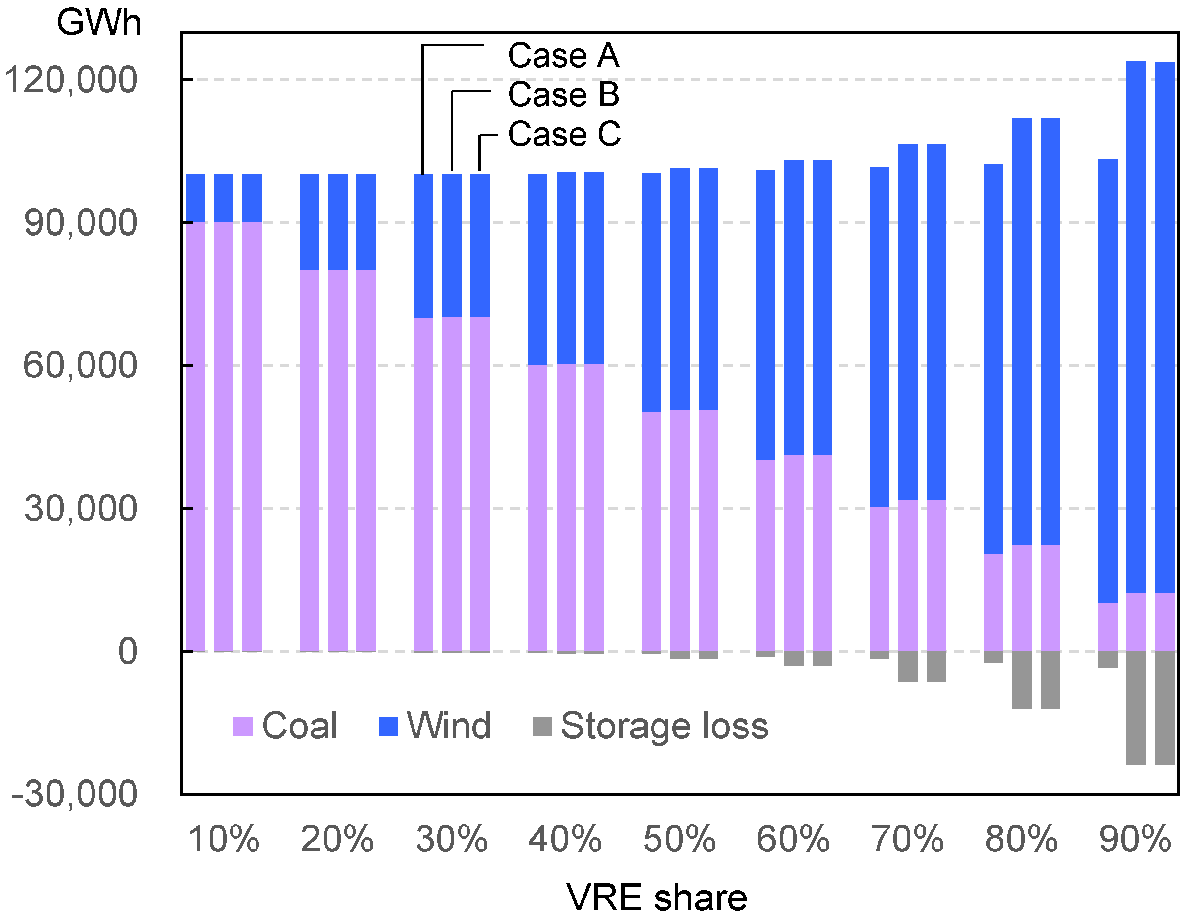
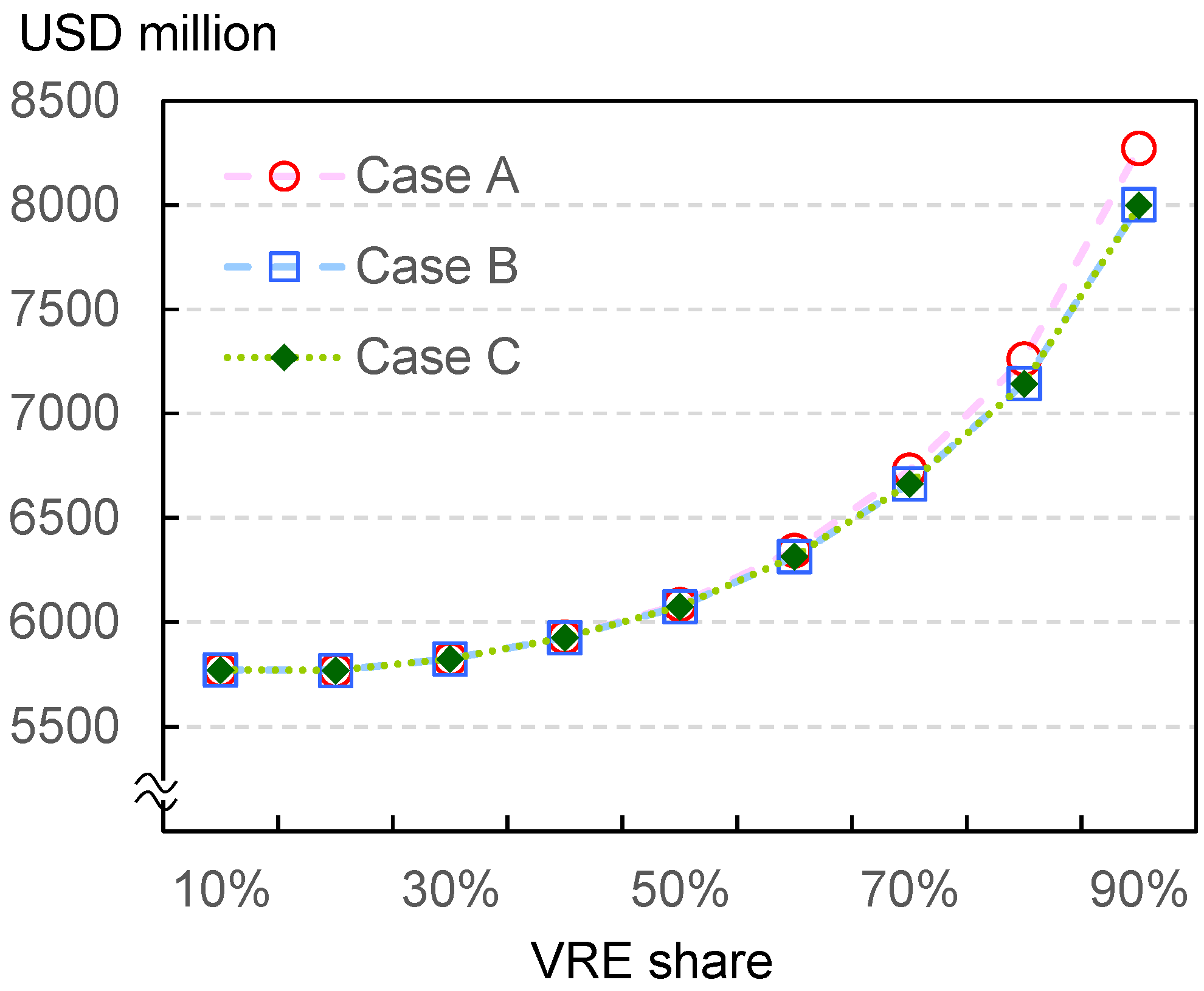
Case A is a case in which coal power output is limited with carbon prices or construction limits, while in Case B, wind power is promoted by strong policy measures, and Case C is an intermediate case. Detailed discussions for these cases are given in Appendix A. In Case A, the value of demand, i.e., the total revenue to the power suppliers, is larger than the total cost, while in Case B, the value of demand is smaller than the total cost, and the gap is compensated by policy costs, such as feed-in-tariff (FIT) bills. As such, electricity markets are in quite different situations for the three cases, but the obtained total cost does not differ much as shown in Figure A3.
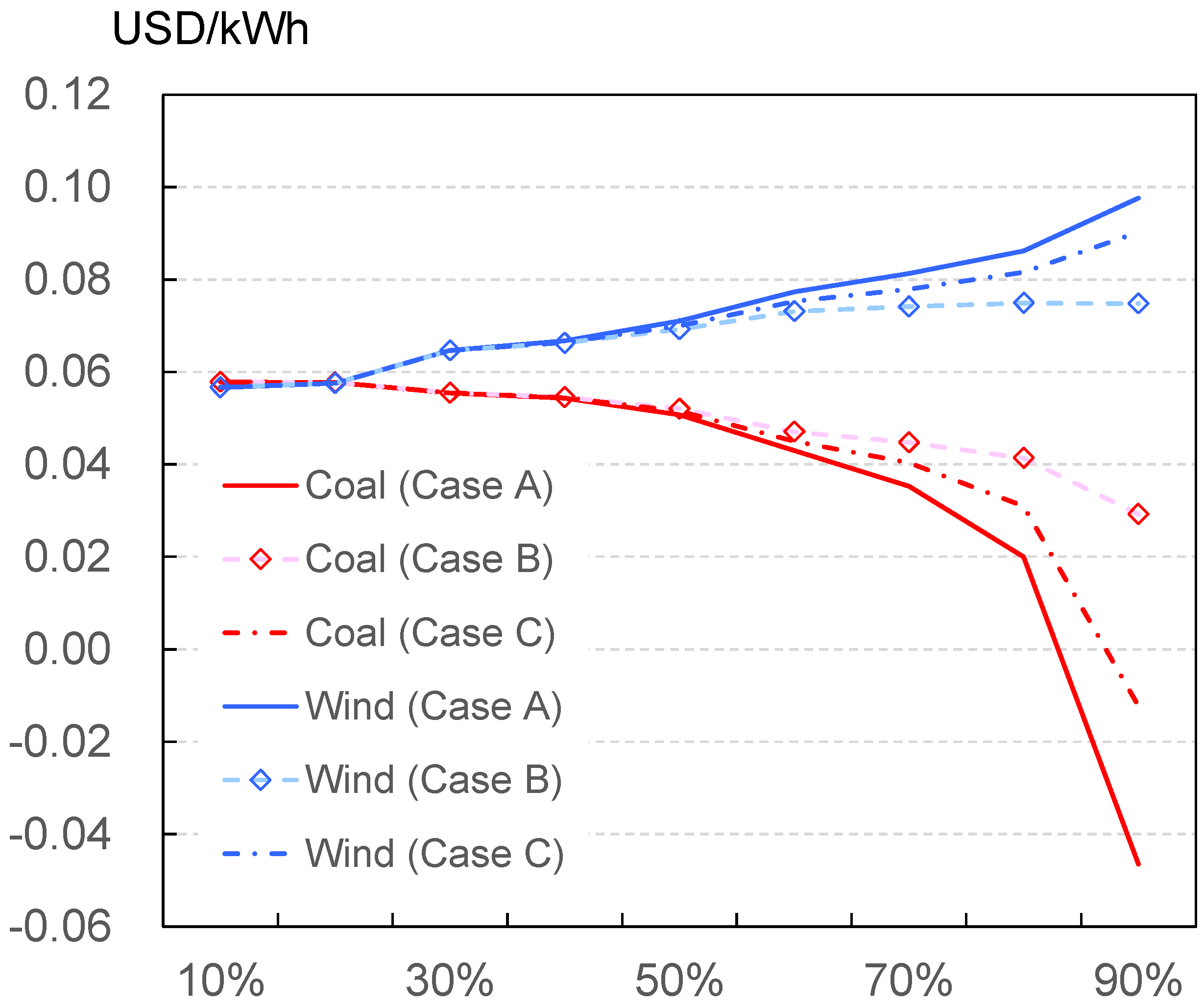
Figure 2 presents the system LCOE_HUE of coal and wind power generation for Cases A–C. We can see large differences in system LCOE_HUE for different cases, although the actual deployment of the technologies is very similar.
By definition, in Case A, in which wind power is not constrained, the system LCOE_HUE of wind is identical to the unit value of demand, which can be calculated by dividing the total value (see Appendix A and Figure A1) by the total annual demand of 10,000 GWh. Similarly, in Case B, the system LCOE_HUE of coal equals the unit value of demand. In Case A, because of the very high value of the coal, the system LCOE_HUE of coal can take even negative numbers with high VRE shares. In Case C, system LCOE_HUE stands in between Cases A and B, as this case exploits constraints for both coal and wind power output.
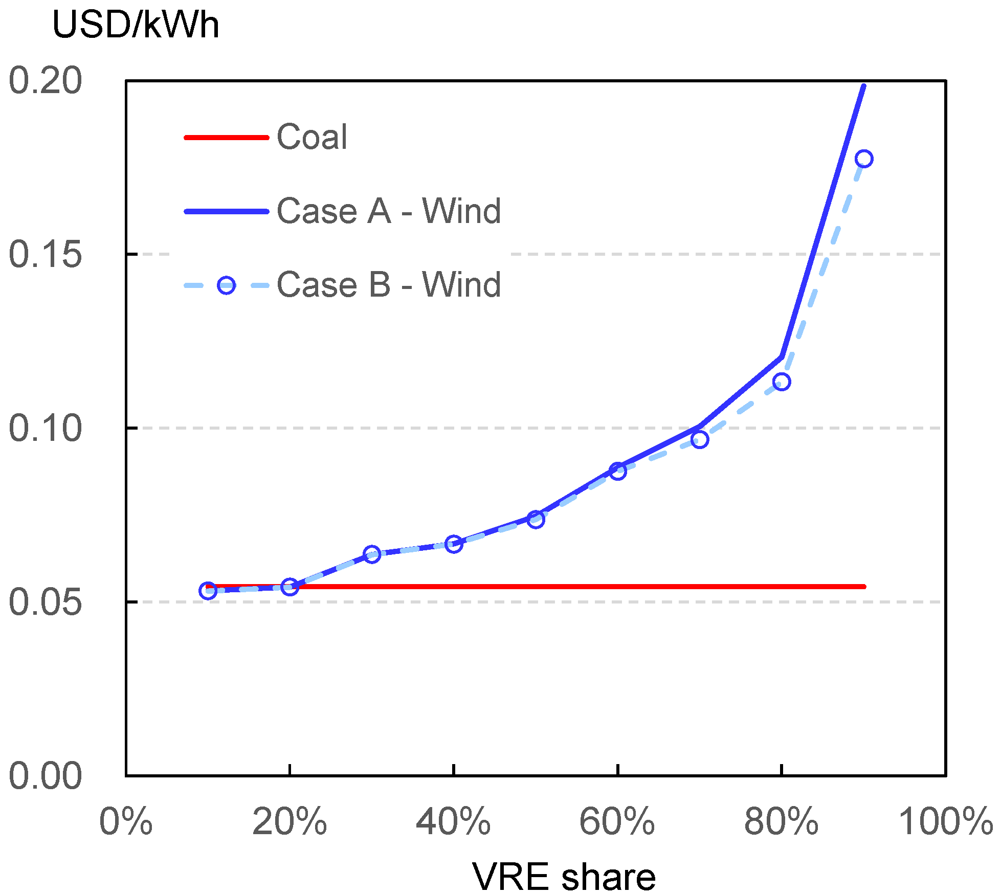
In contrast, Figure 3 shows relative marginal system LCOE for Cases A and B, selecting coal power generation as the reference technology. The number for coal is constant by definition, while that for wind rises sharply, with the increasing share of VRE. At the 90% penetration level, wind takes a number 3.6 times and 3.3 times that of coal, in Cases A and B, respectively.
We can see both similarities and dissimilarities between system LCOE_HUE (Figure 2) and relative marginal system LOCE (Figure 3). First, both metrics take the same numbers for coal and wind at the optimal point of 22%. Second, the difference between coal and wind expands rapidly along with the increasing share of VRE.
In contrast, we see a large difference for the gap between Cases A and B. In line with the slight gap for the total cost (see Figure A3), relative marginal system LCOE, in Figure 3, is slightly lower for Case B than for Case A. However, we find large discrepancies for system LCOE_HUE, as is explicit in Figure 2. This is because system LCOE_HUE is dependent on the value of demand vL, which differ largely for Cases A and B. At the same time, from a mathematical point of view, we can also show that this is because this metric does not consider the coefficient Ri.
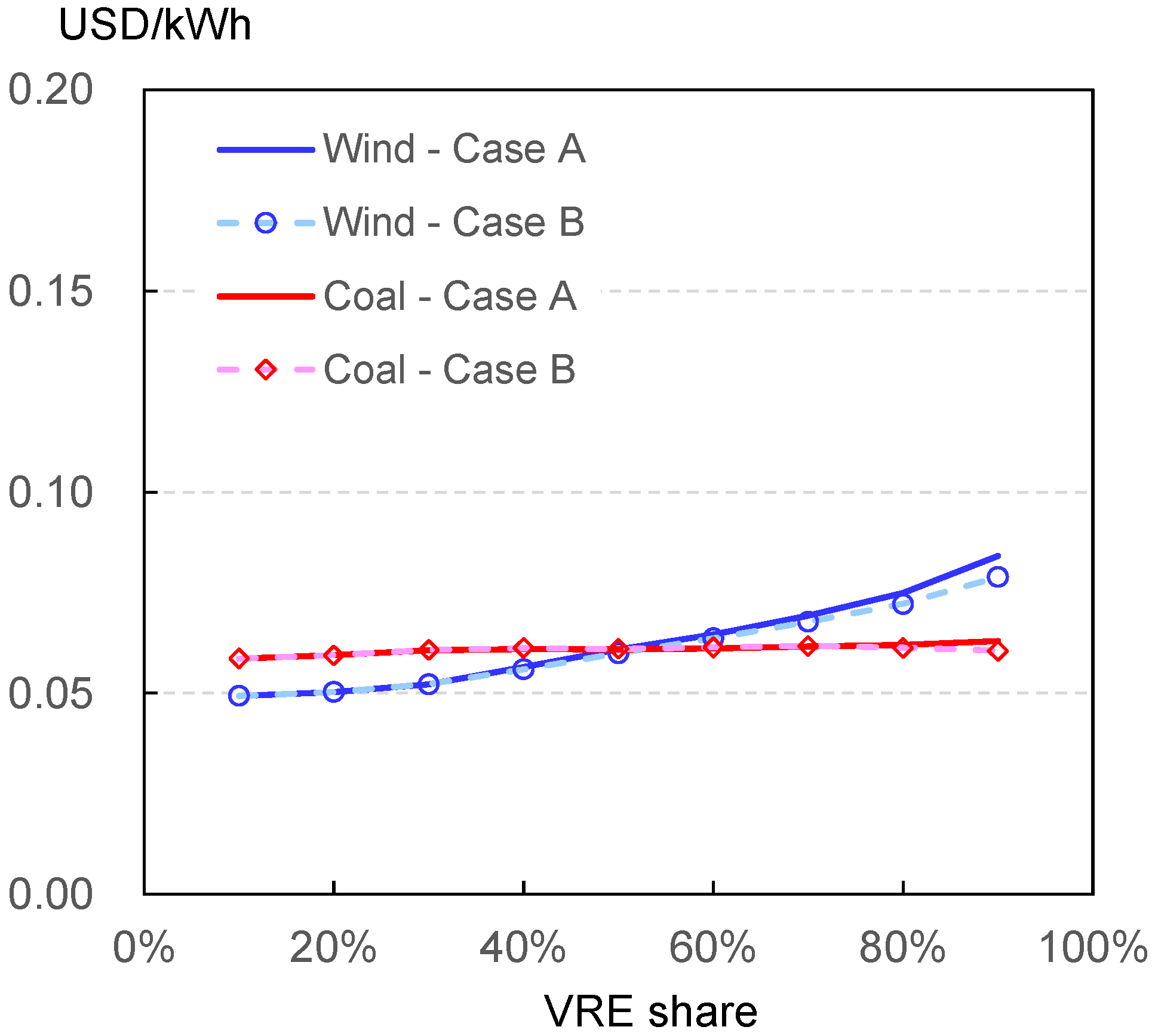
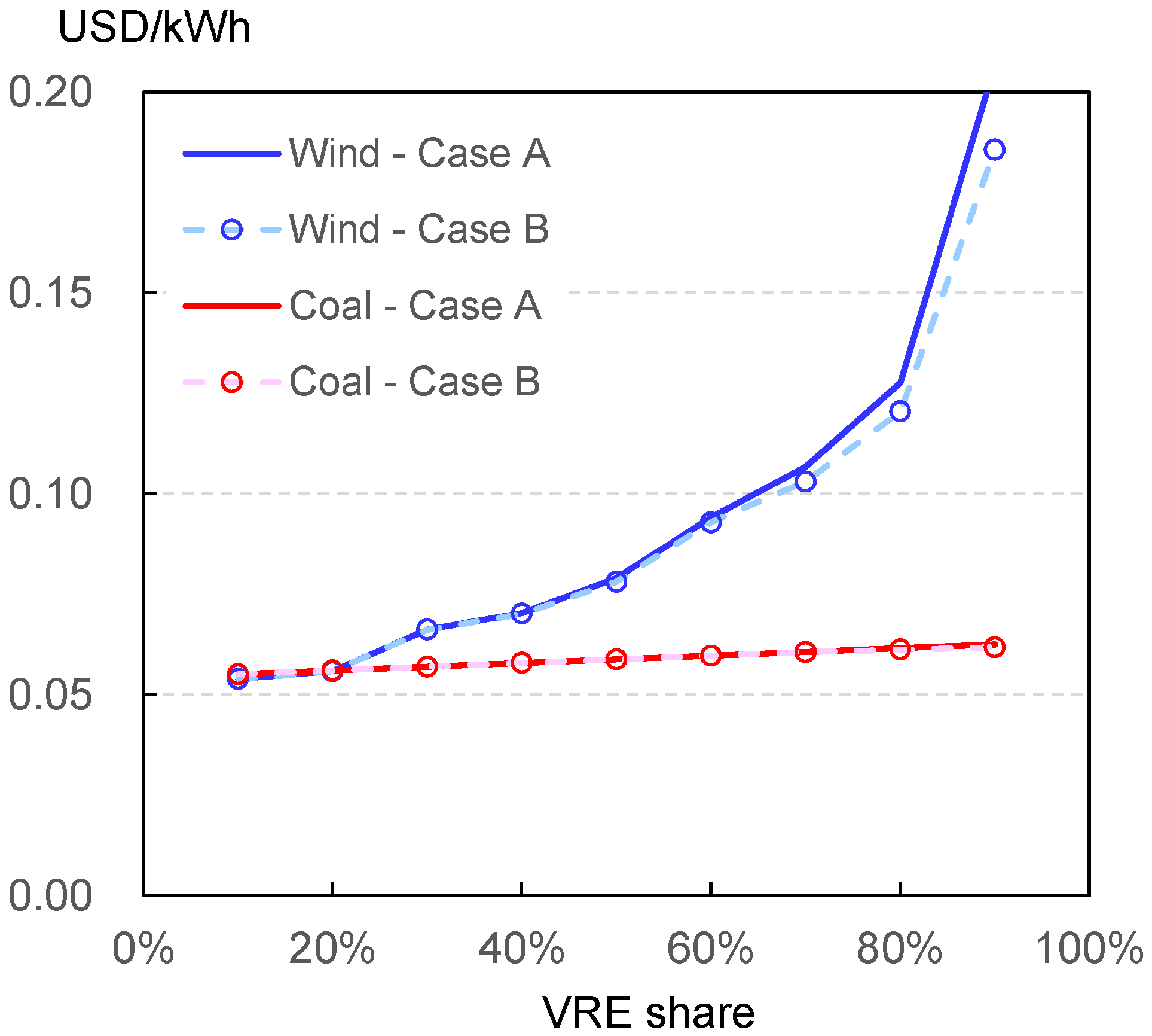
Figure 4 and Figure 5 show average system LCOE and marginal system LCOE for wind and coal, for Cases A and B. Case B shows slightly smaller costs than Case A, in line with the slight differences in the total system cost. Notably, the point where both sources have an equal average system LCOE stands at around 50%, compared to 22% for relative marginal system LCOE. Generally, if the cost of a technology increases with a convex function with respect to VRE penetration, average system LCOE rises more slowly than marginal system LCOE.
These results would imply the following conclusions: As the increase in the average system cost is relatively small, the net social impacts of achieving high VRE shares would also be small, if it is achieved by adequate policy measures. In fact, Figure 4 implies that we could promote VRE diffusion at least to 50% without any significant additional costs.
However, as is widely known, economic equilibrium is determined by marginal costs rather than average costs. The calculation results would imply that strong policy measures would be required to achieve VRE shares over 22%, and achieving very high VRE shares could be very challenging. Therefore, we can see that the illustration of average and marginal system costs shows very different pictures. Estimating both metrics would be useful for realistic policymaking.

2.3. Calculations for a Real System: Japan’s Decarbonised Power Sector in 2050

This subsection illustrates how the methods explained in previous sections can be applied to actual systems, taking the example of Japan’s power mix in 2050 investigated by previous studies [18,19,20]. These studies divided Japan, excluding Okinawa, into nine regions and computed the total system costs using an LP model with a 10-min resolution. The technologies assumed here include VRE (solar PV, onshore wind, and offshore wind), dispatchable renewables (hydro, geothermal, and biomass), nuclear power, and a zero-emission thermal power generation, which could be either thermal power using imported hydrogen, or that with the carbon capture and sequestration (CCS) technology. The upper limits of VRE are set according to the Ministry of the Environment (2019) [54]. Although we can deploy a large amount of onshore wind and solar PV, in cases with little availability of thermal power generation, these technologies reach the upper limits and offshore wind, which is assumed to be more costly, also starts to be exploited. Existing nuclear power plants are assumed to continue operation until their extended lifetime of 60 years, which implies that we can assume a 25.5 GW nuclear capacity at the maximum. For exact details of the assumptions, the reader is referred to Matsuo et al. (2018) [19].
For the current study, the model is simplified to calculate system LCOE in 2050 in Japan as follows, primarily because of the large machine time required, especially for computing the allocation of integration costs:
  • Japan is regarded as one region, or divided into three (Hokkaido, Tohoku, and other areas) or five (Hokkaido, Tohoku, Tokyo, Western Japan excluding Kyushu, and Kyushu) regions, rather than the nine regions in Matsuo et al. (2018) [19].
  • The calculations focus on five types of power generation: Zero-emission thermal, nuclear, onshore wind, offshore wind, and solar PV. Power output from other technologies (hydro, geothermal, and biomass) are fixed and subtracted from power demand in advance of the calculations. The zero-emission thermal power generation in region 3, including Tokyo, with an LCOE of 11.2 JPY/kWh at the maximum load factor of 80%, is adopted as the reference technology.
  • A model with an hourly resolution, rather than one with a 10-min resolution, is used, only for simplicity.
  • The “lower” and the “medium” cost assumptions in Matsuo et al. (2018) [19] are used for renewables and zero-emission thermal power, respectively. Hydrogen storage is also allowed, along with lithium-ion batteries.
In addition, this study considers two types of demand flexibility. First, the effects of electric vehicles (EV) have been considered, based on the literature. Specifically, driving patterns of Japanese automobiles are estimated, and analyzed using a clustering method, according to the “Road Traffic Census Vehicle Origin and Destination Survey” data. Then, it has been assumed that EV can charge electricity when they stay in the house or in the office, which leads to demand flexibility. Moreover, it is also assumed that EV can discharge power to the grid to meet other power demands and minimize the total power system cost including the EV. In all cases, a “single-day” constraint was set. That is, the state of charge in the beginning of a day should be the same as that in the end of the day. We should note that to achieve these full flexible operation, deliberate design of electricity markets, as well as strong policies to develop the infrastructure, would be required. Here, the model assumes that 44 million EV are introduced in 2050, which amounts in total to a battery capacity of 437 GWh. For more details on EV modelling, the reader is referred to Iwafune et al. (2019) [55].
This study also considers demand flexibility by heat pump (HP) heaters. Here, the assumed water heating demand of 34 TWh can be changed flexibly within a day, with the single-day constraint as described above.
Table 1 shows the case setting.
Case 1 is a case in which demand flexibility is not considered, although the deployment of Li-ion batteries and hydrogen storage systems are considered according to Matsuo et al. (2018) [19]. In Case 2, the cost of batteries is assumed to decline to the half of the standard case. Case 3 assumes that hydrogen storage systems are not allowed, to explore a case with less flexibility. Note that in normal cases, batteries and hydrogen storage systems are used for stabilizing short-term and long-term fluctuations of VRE output [20].
Case 4 assumes demand flexibility by EVs, and Case 5 considers VtoG as well. Case 6 considers demand flexibility with HP, and Case 7 considers full flexibility with EVs and HP. In standard cases, meteorological data are taken from actual data for 2017, which has been selected as a typical case from calculations using data from 2012 to 2017 for Case 7. Note that as the exchange rate is around 126 JPY/USD as of early 2022, 1 JPY/kWh is roughly equivalent to 0.8 U.S. cents/kWh.

3. Results and Discussion

3.1. Three- and Five-Regional Models

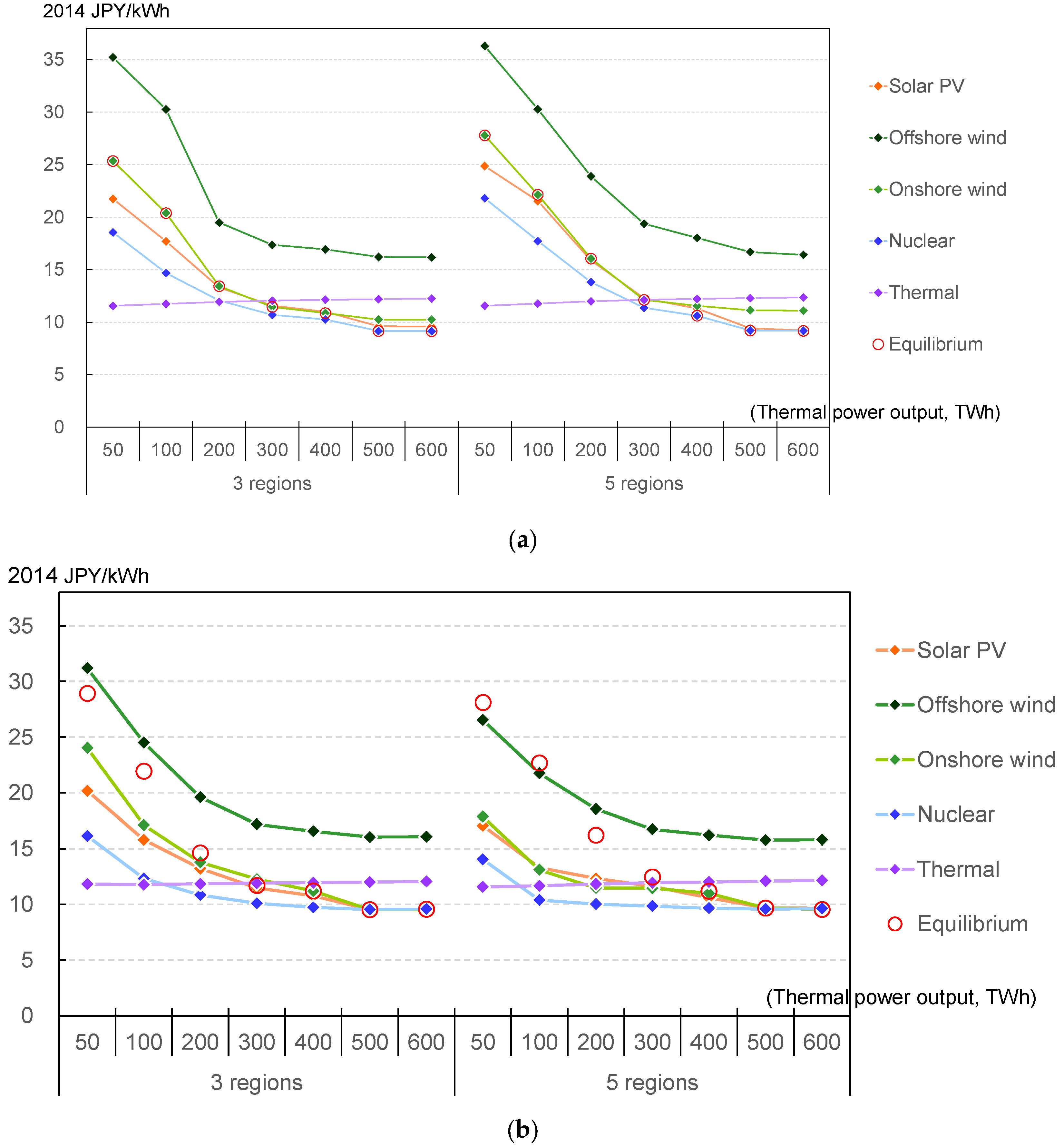
Figure 6 show the marginal system LCOE for the three- and five-regional models, for Case 7 with demand flexibility (2017 data) [56]. Note that while previous Figure 2, Figure 3, Figure 4 and Figure 5 present VRE share for the horizontal axis, Figure 6 adopt the annual output of zero-emission technology (total of the three or five regions), following Matsuo et al. (2018) [19]. Thus, the left-hand side of the charts exhibit higher VRE penetration. As the assumed total annual power demand, including intraregional transmission and distribution losses, is 1044 TWh, a thermal power generation of 200 TWh roughly corresponds to the thermal share of 20%. As each technology has different marginal system LCOE for different regions, the maximum and the minimum values are presented in Figure 6.
As emphasized in Section 2, marginal system LCOE take the same value, shown by red circles, for all the technologies that are not constrained. Marginal system LCOE lower than the equilibrium value indicates that the technology is constrained by upper limits in the region, while that higher than the equilibrium value implies that the technology is constrained by lower limits (only for hydrogen thermal power in this model), or it is not introduced in the region because of the high costs. Thus, offshore wind is not introduced in at least one of the three/five regions, as shown in panel a (maximum) of Figure 6. Panel b (minimum) shows that offshore wind has not been introduced in any of the regions for the three-regional model and is introduced in at least one of the regions with thermal power output smaller than 200–300 TWh for the five-regional model. Overall, the maximum value of marginal system LCOE is larger, and the minimum value is smaller, for the five-regional model than for the three-regional model. This implies that higher regional resolution enables us to estimate regional differences in market values more precisely. At the same time, we observe that the equilibrium values are higher for the five-reginal model than for the three-regional model; they intersect with the marginal system LCOE of hydrogen thermal power at 200–300 TWh and 300–400 TWh for the three-regional model and the five-regional model, respectively. These points of intersection roughly correspond to the power generation mix that minimizes the total cost C.
The marginal system LCOE of nuclear power also increases along with declining thermal output, because of the lower load factors, and the relative inflexibility of nuclear power, and exceeds thermal power below 100 TWh.
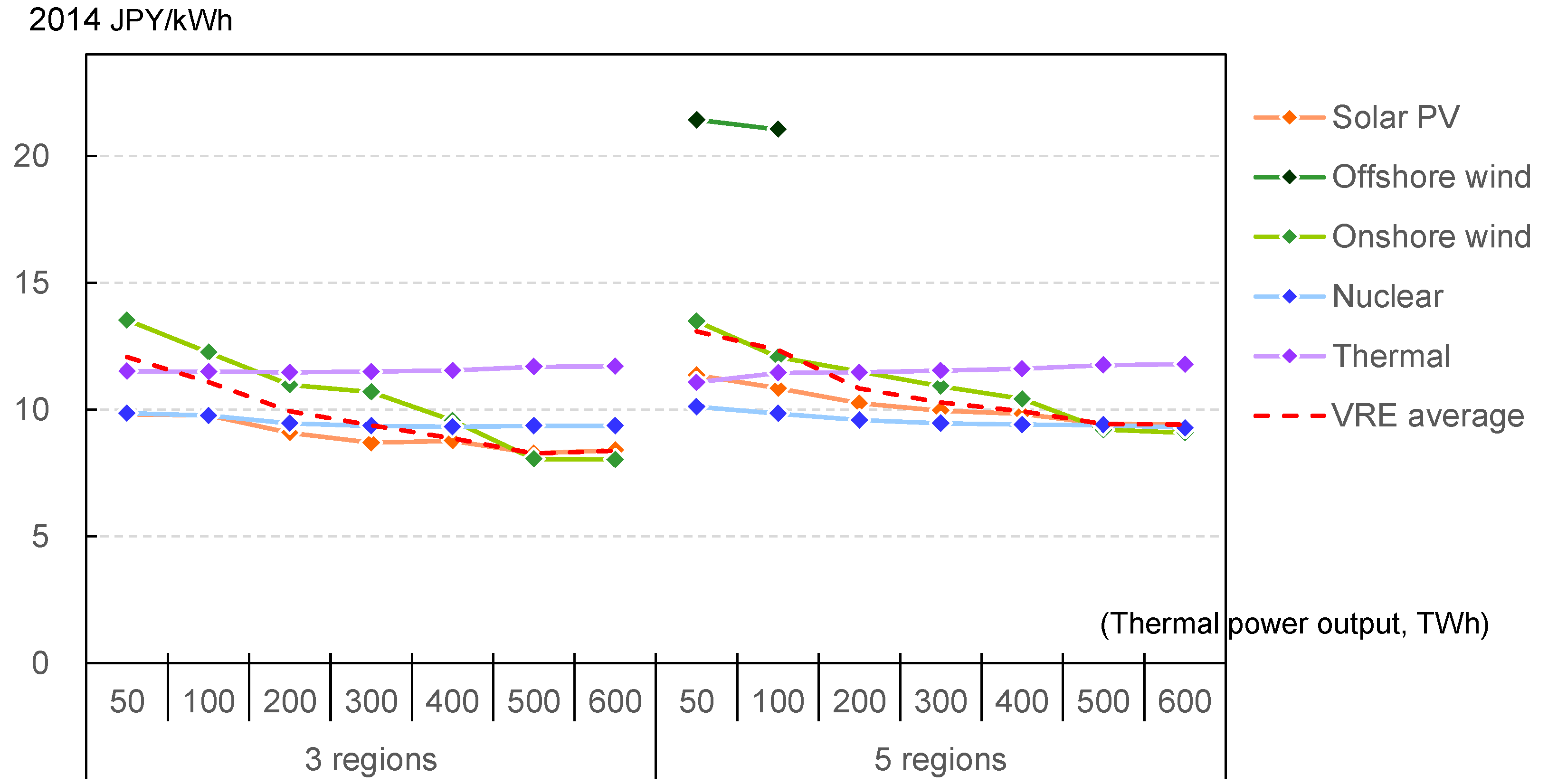
Figure 7 exhibits average system LCOE for each technology. As thermal output declines, the average system LCOE of solar PV and onshore wind increase gradually. Solar PV exhibits much smaller average system LCOE than wind power, implying that the capacities reach the upper limits with relatively large thermal output. The rise in the average system LCOE of nuclear power is even slower, because of high values of firm capacities with high VRE penetration.
The average system LCOE of VRE intersects with that of thermal power at points with smaller thermal output. Solar PV is always lower than thermal power in the three-regional model and intersects at around 50 TWh in the five-regional model, while onshore-wind intersects with thermal power at around 200 TWh. The results imply that the total system cost increases only moderately with very small thermal outputs (i.e., with very high VRE outputs) under the assumption adopted here.

3.2. Effect of Demand Flexibility and Meteorological Condition

Table 2 shows marginal system LCOE (maximum and minimum) and average system LCOE for Cases 1–7, with a thermal power generation of 50 TWh. Meteorological condition (year 2012 to 2017) for Case 7 affects marginal system LCOE greatly, with that for solar PV and onshore wind fluctuating with a standard deviation of 1–2 JPY/kWh (0.8–1.6 cent/kWh). As shown in Matsuo et al. (2020) [20], the cost of achieving very high shares of VRE is determined by the duration of “windless and sunless” periods within the year. On the other hand, average system LCOE changes only marginally, with a standard deviation of 0.2–0.3 JPY/kWh (0.16–0.24 cent/kWh).
The larger the number of regions (1, 3, and 5), the larger the maximum of marginal system LCOE, and the smaller the minimum. This would emphasize the importance of detailed geographical modeling, reflecting the feature of each region. Again, the difference in average system LCOE is much smaller.
Compared to Case 1, in which demand flexibility is not considered, average system LCOE is smaller for Case 7, in which demand flexibility is fully taken into account. This clearly shows that demand flexibility can contribute to declines in the cost of VRE. Declines in average system LCOE is larger for solar PV at 1.3 JPY/kWh (1.0 cent/kWh), than for onshore wind at 0.4 JPY/kWh (0.36 cent/kWh). This implies that the demand flexibility considered here, that is, HP and EV, adapts better to variation in solar PV output, which fluctuates within a day. In Case 3, in which EVs are assumed to provide demand flexibility but not supply stored electricity to the grid, declines in marginal system LCOE are much smaller. In Case 2, in which the cost of batteries is assumed to decline more rapidly, declines in average system LCOE are larger for wind at 1.6 JPY/kWh (1.3 cent/kWh) than for solar PV at 1.2 JPY/kWh (1.0 cent/kWh), in contrary to Case 7.
Changes in marginal system LCOE are more complex. In Case 2 with low battery costs, marginal system LCOE of VRE are significantly smaller than Case 1, which implies that low battery costs facilitate the diffusion of VRE. On the contrary, in Case 3, in which hydrogen storage is not considered, marginal system LCOE are larger. The effects of demand flexibility, such as EV and HP, are mixed. For example, in Case 7, marginal system LCOE for solar PV is slightly smaller than Case 1 by 0.6 JPY/kWh (0.5 cent/kWh), while that of onshore wind is slightly larger by 0.2 JPY/kWh (0.16 cent/kWh).
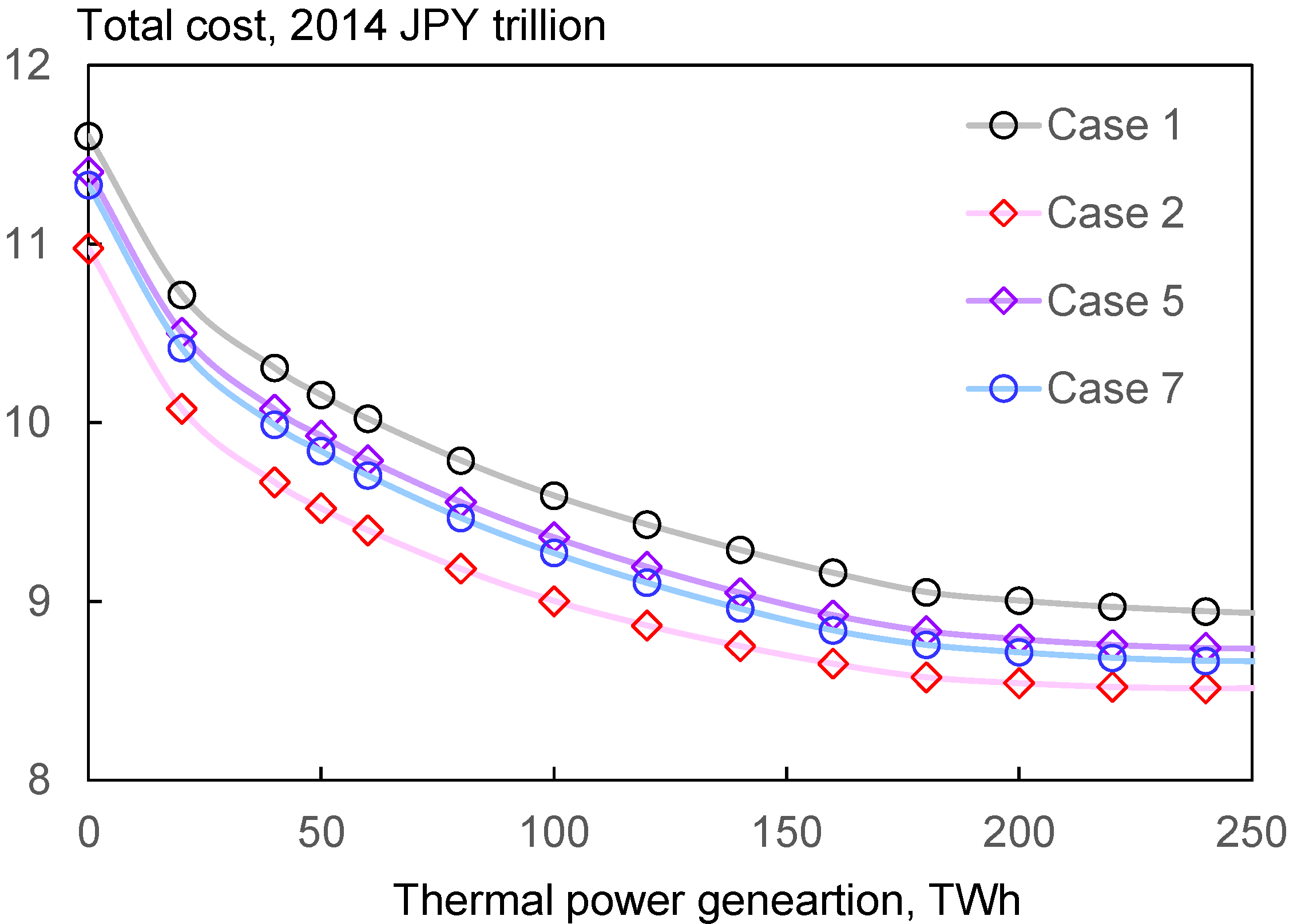
Slight increases in marginal system LCOE does not mean that demand flexibility hinders VRE diffusion. Figure 8 plots the objective function (total system cost) versus thermal power generation for Cases 1 (no demand flexibility), 2 (no demand flexibility with low battery costs), 5 (demand flexibility by EV), and 7 (demand flexibility by EV and HP). We can see that cost declines are the largest for Case 2, while we also observe cost declines for Cases 5 and 7. However, the slope of the curve at thermal power generation of 50 TWh is steeper for Case 7 than Case 1, which may lead to higher marginal costs for Case 7. As the cost hikes under very high penetration of VRE are mainly caused by the duration of windless and sunless periods which can extend to several days or weeks [20], the effects of EV and HP may be smaller with extremely high VRE shares, because of the single-day constraint. However, we should note that this does not mean that demand flexibility does not contribute to reducing the total cost.

4. Conclusions

In this article, the author proposed several metrics to estimate the economics of power sources under a high penetration of VRE, after reviewing past studies presenting similar metrics. He then illustrated these metrics using simple LP models. An important point to note is that, although average and marginal costs measure the economics of the power sector from quite different perspectives, and yield complementary implications, prior studies did not make a clear distinction between these two notions, or instead considered only one of them [5,14,16,17]. In the examples in this study, the average system LCOE of VRE intersects with that of thermal power generation at relatively high VRE shares, namely 50% for the two-technology model and 50–60% (thermal shares of 10–20%) for the Japan model, which would imply that high VRE shares could be achieved without very large net economic damage. In contrast, the marginal system LCOE intersects at significantly lower shares, at around 20% for the two-technology model and around 30% (thermal shares of 30–40%) for the Japan model, which highlights the difficulty, or the necessity, of strong policy measures, to achieve high VRE shares. With the Japan model, the difference in the marginal system LCOE between thermal and VRE (onshore wind or solar PV) expands to 6–16 JPY/kWh (5–13 cent/kWh) for the case with a thermal output of 50 TWh, which shows a sharp contrast with the difference in the average system LCOE of 1–2 JPY/kWh (0.8–0.16 cent/kWh).
The metrics presented in this study are more precise and policy-relevant than similar ones in past studies, given that marginal system LCOE can be regarded as an extension of system LCOE_HUE by Hirth et al. (2016) [16] to more general cases with storage and transmission losses. It also has the property of “separability”. Therefore, it can be used for the comparison of marginal costs in different countries/regions.
Despite these significant differences, the most important implications of this work are similar to those already implied by Hirth et al. (2016) [16] and other related studies, with possible underestimation of the marginal costs of VRE by system LCOE_HUE, in special cases as shown in Figure 2. At the optimal point, all the unconstrained power sources take the same marginal system LCOE. In other words, different marginal system LCOE indicates that the sources are constrained differently. As such, we can say that marginal system LCOE is a metric that measures the value of constraint, or the distance from the optimal point, caused by natural, political, temporal, or locational constraints.
This sets forth the necessity of conceiving new notions of power generation costs by technology. No single value exhibits the cost of a technology. However, the “cost” of the technology changes depending on the actual energy mix. Generally, the cost of a technology is low when it is not deployed much, and it increases with penetration into the system. In the examples shown in this study, these cost increases are caused by such effects as declines in load factors, declines in unit values because of the cannibalization effect, and increases in storage and transmission requirements. In cases that are more realistic, many other factors, such as the rise in construction costs because of siting limitations, or public acceptance issues, could also boost the cost of the technology.
We can think of multiple measures to reduce the total cost associated with mass introduction of VRE. If the cost of batteries, or more generally, the costs for securing grid stability, are reduced, then the average and marginal system LCOE of VRE decrease. Demand flexibility, such as EV and HP, can also reduce the total cost. However, the calculation results also suggest that their effects on marginal system LCOE are mixed, and even in case it decreases, the gap between VRE and flexible thermal power may not be filled. These results underscore the importance of pursuing demand flexibility measures. Moreover, the mitigation of the LCOE of VRE itself can contribute greatly to reducing integration costs, and to enhancing the cost-effective introduction of non-carbon energies. At the same time, the results would also imply the unexpectedly high hurdles to achieve very high shares of VRE, because marginal system LCOE may not be reduced much, even if we deploy demand flexibility measures to a considerable extent. If this is the case, utilizing other types of low-carbon energies, such as zero-emission (or low-emission) thermal power, should also be an important option to achieve carbon neutrality.
We should also note the limitations of the metric designs and the calculations presented in this work: As for the metrics, they are designed to capture the economics of “greenfield” markets. To simulate real “brownfield” markets, different frameworks might be needed. Although several studies have investigated brownfield markets for 2030 [57], we must say that the theoretical framework has not been sufficient.
In addition, demand side modeling also has a great room for improvement. The rapid development of energy systems, e.g., digitalization and electrification, may have unexpected effects that have not been covered in this study. Identifying relevant issues and estimating their impacts should be an important part of future works.
The insights obtained in this study would imply the necessity of aiming for a “well-balanced energy mix” regarding decarbonized power systems in the future. Traditionally, the term “energy mix” has been related to the optimal deployment of dispatchable power sources, such as thermal, nuclear, and hydro power. The new “energy mix” would refer to the optimal mix among multiple decarbonized power sources, including various types of dispatchable and intermittent renewable energies, nuclear power, and zero-emission thermal power. Depending on only a small part of them would lead to higher marginal costs, or larger risks related to energy security or public acceptance issues. From this perspective, differences in LCOE only partly represent differences in the distance from the optimal point, which is also affected by how rapidly the marginal cost increases with the penetration. In this regard, while LCOE is a metric that shows the initial level of cost competitiveness, we may be able to design another simple metric that indicates the velocity of cost increases. However, such changes in costs are supposed to be heavily dependent on specific power systems, and the actual designs of such metrics are beyond the scope of the current study.

Funding

This research was funded in part by the Environment Research and Technology Development Fund (JPMEERF20212004) of the Environmental Restoration and Conservation Agency provided by the Ministry of Environment of Japan.

Institutional Review Board Statement

Not applicable.

Informed Consent Statement

Not applicable.

Data Availability Statement

Not applicable.

Conflicts of Interest

The authors declare no conflict of interest.

Appendix A. Additional Discussion on System LCOE_HUE: Costs and Values

This Appendix illustrates the concept of system LCOE_HUE in a system defined by the simple model shown in Appendix D. This model assumes that an annual demand of 10,000 GWh is met by a conventional technology (coal-fired power generation) and VRE (wind power generation) and calculates the cost optimal mix of the two technologies using the LP method. It also assumes a storage technology and selects between two options, i.e., power storage or curtailment, when the wind output is larger than the demand. As we assume electricity storage to cause energy losses, the following equation holds: (Coal power output) + (Wind power output) − (Wind power curtailment) = (Total demand of 10,000 GWh) + (Storage losses). Note that the calculation in this Appendix A does not consider the costless technology z, which will be introduced in Appendix B and Appendix C.
In this model, by multiplying the energy balance constraint (Equation (A51)) by its shadow prices p e t , and taking the summation with respect to t, we obtain the balance equation of values, V e L = V e _ x + V e _ y V c h a r g e + V d i s c h a r g e , where V e L = p e t l t , V x = p e t x , and so on. Then, by multiplying the capacity constraint (Equation (A58)) by its shadow price p c , we obtain another balance equation of values, 1 + r V c L = V c _ x + c r V c _ y + s r V s , where V c L = p c max l t , and so on. At each energy mix obtained by the LP simulation, the duality theorem assures that the total cost is equal to the total value:
C = V L + V T + V R = V e L + V c L + V T + V R
where C is the total cost, or the sum of the fixed and the variable costs of all the technologies, which is equal by Equation (A1) to the sum of the total value of demand VL, the value of grid interconnection VT, and the value of the energy mix constraint VR, which is the shadow price of the restriction constraint multiplied by the output of the source that is restricted. As this model does not simulate grid interconnection lines, VT is equal to zero. The total value of demand VL is decomposed into the values related to the wholesale and capacity markets, denoted as VeL and VcL, respectively.
In case we disregard power storage systems, by dividing the balance equations of values by the total output or the total capacity, we obtain equations that the average unit value, veL, equals the weighted average of the unit values ve_i. In this case, the definition of VALCOE by the IEA [14] coincides with that of system LCOE_HUE (Equation (1)). For this reason, the IEA does not consider storage systems “outside” of power sources, but considers complex technologies such as “solar PV + storage” to calculate the effect of storage systems to VALCOE.
Suppose now that we constrain the output of some of the technologies, for example, that of wind power (technology y) in the two-technology system shown in Appendix D. For the unconstrained technology, which is technology x or coal in this case, the cost equals the value in the optimal solution. Thus, subtracting the total cost, equaling the total value, of coal, from Equation (A1), we have
C y = V y + V R
where Cy and Vy are the parts of technology y (wind) in C and VL, respectively. Dividing Equation (A2) by the VRE output y,
c y = v y + v R
where vR is the shadow price (unit value) of the constraint. Putting Equation (A3) into the definition of system LCOE_HUE, i.e., Equation (1), we have
L H U E   y = c y v y + v L = v L + v R
for wind power. For coal, as cx = vx at equilibrium, the system LCOE_HUE equals the value of demand vL.
Equation (A4) is important in understanding system LCOE_HUE; the system LCOE_HUE of an unconstrained technology is always equal to the value of demand. For constrained technologies, the system LCOE_HUE equals the sum of the value of demand and the value of the constraint. This implies that system LCOE_HUE is a metric that measures the difference from the optimal point with respect to each technology. This also holds for VALCOE by IEA (2020) [14], which is a metric essentially identical to system LCOE_HUE.
The discussion here is based on Equation (A1), or the dual theorem of the LP method. As the power system is not always a linear problem, this theorem does not always apply to real markets. However, as long as the problem can be formulated in a differentiable manner, a small fluctuation from equilibrium can be approximated as a linear problem, and the shadow prices of the problem are equal to those of the original nonlinear problem. Note also that the discussion presented in this article, holds true both for linear and non-linear systems, although it is illustrated using linear mathematical models for the sake of simplicity.
Figure A1 shows the costs and the values for the three cases in Section 2.2.4.2, using the model defined by Appendix D. As indicated by Equation (A1), the total value of demand and constraint equals the total cost. With VRE shares larger than the optimal level (22%), Case A takes larger total values of demand than the total costs, with negative values of constraint, while Case B sees larger positive values of constraint with larger VRE shares. The former corresponds to a case in which thermal power generation is restricted with carbon taxes, whereas the latter corresponds to a case in which the government promotes VRE through strong policy measures, such as the feed-in tariff scheme. If the market is complete and greenfield, the subsidy or tax compensate the gap between the costs and the market values. Otherwise, i.e., if the market is brownfield, or some of the power sources are subject to non-market constraints, the power producer cannot recoup the costs from the markets (Case B), which is a simple mathematical representation of the well-known “missing money” problem, or it receives larger revenues than the costs (Case A). Case C stands in between Cases A and B. In this case, both coal and wind power generation are constrained. Therefore, the value of constraint becomes zero.
Figure A1. Total values and costs. (a) Case A; (b) Case B; (c) Case C.
Energies 15 06845 g0a1
Figure A2 and Figure A3 show the total power generation x + y and the total cost C, for the three cases. We can see significant differences between the cases, especially with high VRE shares. For example, if we constrain coal power output at 8273 GWh in Case A, we obtain a wind power output of 92,988 GWh, with total power generation of 103,322 GWh, energy loss (storage and curtailment) of 3322 GWh, and wind share of 90%. In Case B, achieving this 90% share requires a larger wind output of 111,475 GWh, in which case, coal power output and the total power generation stand at 12,386 GWh and 123,861 GWh, respectively. This difference comes mainly from the difference in the values of power sources. At high shares of VRE, the value of coal is very high while that of wind is low. In Case A, which constrains coal power output, the model solves the substitution between wind power output and storage deployment, giving results with small wind output and small losses. In contrast, in Case B, which constrains wind output, the model solves the substitution between coal and storage, to produce results with large coal output and large losses. At the optimal point calculated without power generation constraints, which has a 22% wind share for this model, Cases A and B produce the same result; otherwise, the two cases lead to different states. Case C, which constrains the wind share itself, produces similar results to Case B, as the model can exploit large coal power generation with high values. Thus, Cases B and C result in smaller optimal costs than Case A, as shown in Figure A3.
Figure A2. Total power generation by case.
Energies 15 06845 g0a2
Figure A3. Total system cost by case.
Energies 15 06845 g0a3
Figure A4 exhibits the results of the allocation of the total cost according to the method using the costless technology, as explained in Appendix B.2 and Appendix C.2. Although the largest part of the integration cost is allocated to wind power, a smaller part is also allocated to coal, which implies that the cost increases because of the declines in the load factor of coal power generation to meet the changing demand should be mainly allocated to coal. With high VRE shares, the total cost is slightly higher for Case A than for Case B. In Case B, the LCOE part of wind is larger than in Case A, reflecting the difference in wind power generation, while the integration part is smaller in Case B because of small requirements for storage systems. Note that a primary aim of introducing VRE is to mitigate carbon dioxide emissions. Given that Case A, which directly constrains coal power generation, emits less carbon dioxide than Case B with the same VRE share, Case A should be considered more policy-relevant.
Figure A4. Allocation of the total cost. (a) Case A; (b) Case B.
Energies 15 06845 g0a4

Appendix B. Re-Defining System LCOE—A Simple Case with Two Technologies

This appendix defines and discusses the concepts of marginal and average system LCOE, for a special case with two technologies, and without explicit consideration of electricity losses. Then, Appendix C proposes more general definitions.

Appendix B.1. System LCOE and Optimization of the Power Sector

Suppose a simple system with two technologies, in which x and y denote the annual output of a conventional (coal-fired) technology and VRE (wind), respectively. Assuming that the total annual demand is a constant E, we have
x + y = E
Let C(x, y) denote the total system cost, which can be calculated by LP, or by the mixed integer linear programming (MILP) method, or by any other mathematical optimization. Under condition A5, we try to find x and y that minimize C. This can be achieved by minimizing
L = C λ E x y
in which λ is a Lagrange multiplier. This leads to the following three equations:
L λ = x + y E = 0
L x = C x + λ = 0
L y = C y + λ = 0
Equation (A7) is identical to Equation (A5). Eliminating λ from Equations (A8) and (A9), the optimum condition is
C x = C y
If we could regard C / x and C / y as the system LCOE, or the LCOE with an addition of the marginal integration cost, Equation (A10) would mean that the optimal point is where the system LCOE of both technologies take the same value. The problem here is that these partial differentials cannot be calculated uniquely; C / x refers to the increase in C with a small increase in x, under the condition that y is constant. This assumes that E in Equation (A5) also increases by dE along with x. However, the way in which we increase E is not unique. For example, we can multiply hourly demand et by a constant for all t, or add a constant to et. We can think of many ways to increase the total annual demand E. We should also be aware that the actual states of interest are only those under condition A5, and that varying E is a pure mathematical requirement.
Suppose two cost functions CI(x, y) and CII(x, y), which satisfy CI(x, y) = CII(x, y) = C(x, y) if Equation (A5) holds, and can take different values otherwise. We have
d C I = C I x d x + C I y d y
for CI and a similar equation for CII. Putting Equation (A5), or dx + dy = 0, into Equation (A11), we have
d C I = C I x C I y d x
Similarly, for CII, we have
d C I I = C I I x C I I y d x
As dCI = dCII under condition A5, by comparing the coefficients of Equations (A12) and (A13), we have
C I x C I y = C I I x C I I y
This equation implies that although C / x and C / y cannot be calculated uniquely, the difference between them is defined uniquely. Therefore, if we interpret the optimum condition (A10) as C / x C / y = 0 , this condition is unique.
This is a natural extension of the discussion by Ueckerdt et al. (2013) [23]. To illustrate this, let LC and LV denote the LCOE of the conventional source and VRE, and
C = L C x + L V y + I
where I is the integration cost, which is defined as the total system cost minus the cost components that are proportional to LCOE. With these variables, the optimum condition A10 can be rewritten as
L C = L V + I y I x
Eliminating x using Equation (A5), I = I(x, y) = I(Ey, y) can be regarded as a function of y. Taking the differential of I with respect to y, we have
d I d y = I y I x
We denote the value of Equation (A17) as LINT. Then Equation (A16) can be rewritten as
L C = L V + L I N T
Equation (A18) is essentially identical to the Equation (8) of Ueckerdt et al. (2013) [23], which implies that the system LCOE, defined as the sum of the LCOE of VRE and the marginal integration cost, equals the LCOE of the conventional technology at the optimal point (Figure 1). This is a special case of what is referred to as the “relative marginal system LCOE” in Appendix C. The term “relative” here implies that we can define the marginal system LCOE uniquely if and only if we deform the optimum condition with respect to one technology, as in Equation (A16). Subtracting LINT from both sides of Equation (A18), we have the optimum condition with respect to VRE, and both representations are mathematically interchangeable. However, in many cases, it would fit our intuition better to have a constant system LCOE of the conventional technology and an increasing system LCOE of VRE, than to have a constant system LCOE of VRE and a decreasing system LCOE of the conventional technology.

Appendix B.2. Average System LCOE: Allocation of the Integration Cost

Here, we introduce a hypothetical technology, denoting its annual output as z. Then, we denote the one-dimensional space of x and y, which satisfies Equation (A5), as S1, and denote the two-dimensional space of x, y, and z, which satisfies
x + y + z = E
as S0. S1 is a subspace of S0 satisfying z = 0. As S0 is a two-dimensional space, we can define the cost function C(x, y) on S0, which depends on the cost structure of z. Note that this arbitrariness of the selection of z does not affect the economic assessment in the real space S1, as long as we discuss the differences in partial differentials, as in Equation (A16).
For later discussion, it is convenient to assume that z is a “costless” technology, which has zero fixed and variable costs, with unlimited flexibility. Although this is quite a hypothetical assumption, it is fairly easy to add this type of technology to mathematical models to define C(x, y) on S0.
I now define the “absolute marginal system LCOE” as follows, although a more general formulation will be given later.
L A x = C x
L A y = C y
An exact formulation would be to define the cost function C(x, y, z) in a three-dimensional space, including S0, without condition (A19), and define L A x = C / x C / z uniquely following the discussion in the previous subsection. We then obtain Equation (A20), regarding C as a function of x and y on S0.
Using the absolute marginal system LCOE, we can decompose C(x, y) into two parts, namely, Cx and Cy, which represent the contribution of the conventional technology and VRE, as follows:
C = d C = C x d x + C y d y = C x d x + C y d y C x + C y
The LCOE of each technology can be denoted as L 0 x and L 0 y , but before that, we must define LCOE without ambiguity; the LCOE of a technology can take different values depending on the load factor. I define the LCOE of a technology as calculated assuming the highest possible load factor. In the model shown in Appendix D, for example, it is defined as the value calculated assuming load factors of 80% for the conventional technology and 22% for VRE (wind power). Thus, the total system cost C is decomposed into the part proportional to LCOE, and the remaining integration cost part denoted as I:
C = L 0 x x + L 0 y y + I
The absolute system LCOE L A x is also decomposed as
L A x = C x = L 0 x + I x L 0 x + L I x
where L I x is the absolute marginal integration cost. Similarly, as in Equation (A22), I can also be decomposed into two parts:
I = I x d x + I y d y I x + I y
and the equation C x = L 0 x x + I x holds.
Dividing the allocated cost C′x by the annual output x, we obtain the “average system LCOE” L ¯ x :
L ¯ x C x x = L 0 x + I x x L 0 x + L ¯ I x
where L ¯ I x is the average integration cost. As Equations (A24) and (A26) show explicitly, both the absolute marginal system LCOE and the average system LCOE are expressed as the sum of LCOE and the marginal/average integration cost. These equations will be re-formulated again in a more general manner in Appendix C.
Although Equation (A23) is formally quite similar to Equation (A15), our formulation here defines the LCOE more strictly in terms of the assumed load factor. Figure A5 shows C and I calculated by the model presented in Appendix D, with the condition x + y + z = E (that is, without any deployment of the storage system and without any energy losses). In these charts, the two-dimensional plane parameterized by x and y corresponds to S0, and the line x + y = E on the plane represents the set of real states S1.
Figure A5. Illustration of the total cost C and the integration cost I. (a) C; (b) I.
Energies 15 06845 g0a5
Figure A6 illustrates C in two subspaces of S0, that is, as a function of x with y = 0 and as a function of y with x = 0.
Figure A6. Total cost C and the integration cost I on subspaces y = 0 and x = 0. (a) y = 0; (b) x = 0.
Energies 15 06845 g0a6
As described above, the LCOE of a technology is defined as the levelized cost calculated with the maximum load factor. In case we supply the system only with the conventional technology (that is, y = z = 0), the load factor takes a somewhat lower value. The storage system may also be introduced to cause additional costs. As illustrated in the left-hand side chart of Figure A6, the LCOE of the conventional technology is shown as the slope of the cost function near x = 0, and the difference between C and the dotted line proportional to the LCOE represents the integration cost I.
LCOE depends heavily on the load factor. For example, OECD/NEA and IEA (2020) [5] proposes a sensitivity analysis assuming different load factors, for example, 80% and 50%, to illustrate the effects of operational conditions. In contrast, our definition of LCOE here implies that the cost increases caused by lower load factors are classified as part of the integration cost, rather than of the LCOE. In this context, the integration cost is recognized as the additional cost caused by the inflexibility of each technology. L A x is the change in the total cost with the substitution of 1 kWh of conventional power output with that of the absolutely flexible costless technology, which includes the differences in the values, not only of energy, but also of capacity and flexibility. For this reason, L A x is called the “absolute” marginal system LCOE. As any technology in the real world, whether it is a conventional technology or VRE, has a certain level of inflexibility, I, L I x , and L I y always take positive values in real systems. As illustrated in Figure A5 and Figure A6, I is usually close to zero with small x and y, and increases rapidly as the state moves closer to real systems on S1.
There are at least five important points that must be mentioned here. First, the LCOE of a conventional technology L0x equals the limit lim x 0 C / x y = 0 . That is, the integration cost of a conventional technology is close to zero, and the absolute system LCOE is close to the LCOE around the origin of the coordinates. However, for VRE, this is not always the case. This is because of the capacity constraint, including reserve margins. Should the power demand be met only with VRE and the costless technology, without any real stable technology, the capacity constraint may not be met without additional costs; see Equation (A58) for the model presented in Appendix D. For this model, while lim x 0 C / x y = 0 equals the LCOE of the conventional technology at 5.44 U.S. cent/kWh, lim y 0 C / y x = 0 , equaling 4.84 U.S. cent/kWh, is larger than the LCOE of VRE at 4.50 U.S. cent/kWh, which is dependent on the assumption of the capacity credit of VRE, and which can be regarded as the marginal integration cost that exists even near the origin of the coordinates.
Second, in Equation (A22), the decomposition of C into C′x and C′y is not determined uniquely but depends on the path of integration. This is exactly the problem of allocating costs to each source; if we adopt Path I in Figure A7, we have small C′x (very small I′x) and large C′y. This path corresponds to the allocation in which we have a system only with x in the first place, and then add y, to allocate the related cost increases only to y. On the contrary, if we take Path II, most of the integration cost is allocated to x. Here, I propose a simple linear Path III to allocate the costs to each technology equally.
Figure A7. Integration paths for cost allocation.
Energies 15 06845 g0a7
Through several tests, we can examine that this path yields a fair allocation, without contradicting with our intuition. For example, let us suppose a symmetric case, as shown in the left-hand side chart of Figure A8, in which both x and y represent conventional technologies, or both represent VRE. Our intuition tells us that at point x = y = E/2, C′x should be equal to C′y, and L ¯ x should be equal to L ¯ y . While it is obvious that the linear path from the origin satisfies this condition, other paths do not satisfy it, except for very special winding paths. Moreover, if C is convex in S1, as shown in the left-hand side chart of Figure A8, L ¯ x is larger than L ¯ y if x is larger than y, which also satisfies our intuition.
Figure A8. Test shapes of the total cost C.
Energies 15 06845 g0a8
Another important test is the case in which x and y have exactly the same cost structure, i.e., the same fixed and variable costs, capacity credit, and flexibility. In this case, L ¯ x = L ¯ y must hold at any point on S1 because of the symmetry. Here, I prove that this is the case with Path III in Figure A7:
As x and y have exactly the same cost, C(x, y) can be written as a function of x + y, namely, C(x + y), as shown in the right-hand side chart of Figure A8. This leads to the equation C / x = C / y . As the path is linear, we can assume that y = αx or dy = αdx, with a constant α. From the definition (Equation (A22)), for a point (X, Y) = (X, αX) on S1, we have
C x X ,   Y = 0 X C x d x = 0 α X 1 α C y d y = 1 α C y X ,   Y
This yields
L ¯ x = C x X = C y α X = L ¯ y
This supports the appropriateness of adopting the linear Path III; if the shape of the cost function is convex, as shown in the right-hand side chart in Figure A8, Path IV in Figure A7, which takes larger x than Path III, yields smaller C′x and larger C′y, and Path V with smaller x yields larger C′x and smaller C′y. Thus, these other paths would not yield a reasonable allocation.
Third, can we use other types of hypothetical technologies than costless ones, to calculate the allocation using Equation (A22)? I use the costless technology here because it allows us to measure cost increases caused by the inflexibility of real-world technologies in full range. In fact, L A x in Equation (A24) on S1 take the largest value if we use the costless technology, which is why it is called the “absolute” marginal system LCOE. Moreover, the function C, as shown in Figure A5 and Figure A6, takes the smallest values if we adopt the costless technology for z, and for other technologies, the function C exhibits a larger path than the line with the slope identical to the LCOE. This would imply that with other technologies, we could not decompose C properly into the integration part and the part proportional to the LCOE.
Fourth, as Equation (A10) shows, all the absolute marginal system LCOE take the same number, or more precisely, the differences between the absolute marginal system LCOE of different technologies become zero, at the optimal point. However, average system LCOE does not take the same number at the optimal point, except for special cases, such as that shown by Equation (A28). This follows the general principle of economics that the optimal point is determined by marginal costs, rather than by average costs. In our case, if the LCOE of VRE is smaller than that of conventional sources, the average system LCOE usually take smaller numbers for VRE than for conventional sources at the optimal point.
Fifth, although it may be theoretically appropriate to discuss with absolute marginal system LCOE, it can take very large values, as it measures cost increases caused by inflexibility in full range. Realistically, in many cases, it would be more reasonable to use the LCOE part and the difference in the integration part, as in Equation (A16). In the current two-technology system, we can choose the conventional power generation as the “reference” technology, and define the “relative marginal system LCOE” as
L R x = L 0 x
L R y = L 0 y + I y I x
Again, although L R x   and L R y can be calculated using the costless technology, or using any other hypothetical technologies, the values do not depend on this arbitrariness. The relative marginal system LCOE defined here is essentially the same as the marginal system LCOE defined by Reichenberg et al. (2018) [17], with a slight difference from our definition, in that Reichenberg et al. (2018) [17] adopt their “thermal LCOE,” which is the total system cost without VRE, divided by the total power generation, as the constant in the right-hand side of Equation (A29).
L R x equals L R y at the optimal point. Although we can choose any power source as the reference technology, it would be reasonable in many cases to select a technology with high flexibility, because of several reasons as described in Appendix C.

Appendix C. Re-Defining System LCOE—General Case with Multiple Technologies and Electricity Losses

Appendix C.1. Relative Marginal System LCOE
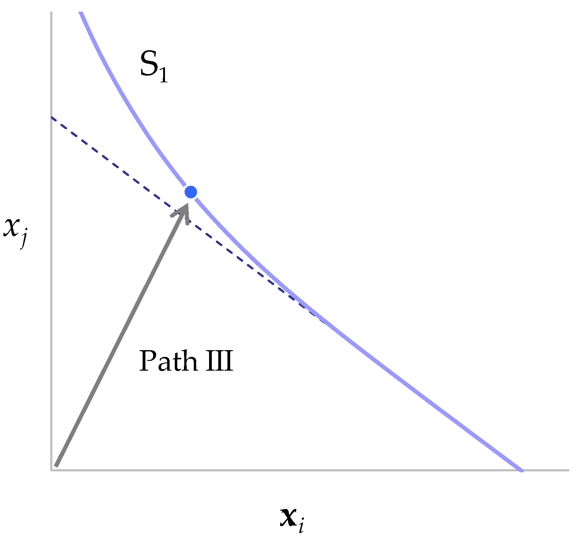
When we extend the discussion in Appendix B to more realistic systems with multiple power sources, we must consider the changes in the total power output due to energy losses. With high penetration of VRE, we generally have large excess electricity, which is partly curtailed. This results in smaller power output after curtailment than the total power generation. We must also consider transmission and charge/discharge losses that would enlarge the need for power generation. For these reasons, we generally have larger power generation with higher VRE shares. Equation (A5) is a special case without these energy losses.
Let us assume a system with n technologies. Denote the annual power output of technology i (i ∈ [0, n]) as xi, and the total annual energy loss as T. Unlike Equation (A5), xi can vary relatively unrestrictedly, because it is at least possible to assume a state with very large power generation and very large storage losses. We assume here that all xi can be determined uniquely by optimization calculations.
Another important point is that the state of the system can vary depending on how we constrain it, as exemplified in Section 2.2.4.2. For example, if we fix xi as x i = x ^ i for i ∈ [0, n − 1], xn is also determined by optimization. We can calculate the optimal state fixing xi for i ∈ [1, n], only to obtain x0 that is different from x ^ 0 . This corresponds to the fact that subsidizing VRE and levying a carbon tax on thermal power would produce similar, but not the same situations in the real world.
We assume here that we can define the total cost C, as well as the energy loss T, on a n-1-dimensional space of real states S1, by choosing one unconstrained technology i0, and optimizing the system fixing xi for i other than i0. C, T, and any other function on S1 are primarily defined as functions of xi for i other than i0. However, we can also regard them as functions of any n − 1 combinations of xi, other than xi* with one i* ∈ [0, n], as it is possible to calibrate xi* so that x i 0 takes any intended x ^ i 0 . As stated above, the selection of i0 is dependent on the policy measures to realize the state and can exert non-negligible effects on the costs of power sources.
Now, without loss of generality, we select x0 as the annual output of the “reference” technology, regarding x0, C, and T as functions of annual output of other sources, that is, x1, x2, …, xi. The unconstrained technology i0 may or may not be identical to 0. Here, instead of Equation (A5), we have
i 0 x i = E + T
The set of xi that satisfies Equation (A31) makes the real-state space S1. Considering the annual output of the costless technology xCL, we can think of a space S0 that satisfies
i 0 x i + x C L = E + T
As Figure A9 shows, S1 forms a curved surface in S0.
Figure A9. Case with electricity losses.
Energies 15 06845 g0a9
Similarly, as the discussion in Appendix B.1, using a Lagrange multiplier, we can formulate the optimum condition in S1 as
C x i 1 T x i C x 0 = L i R i L 0 = 0
for all i, where R i = 1 T / x i and
L i = C x i = L 0 i + I x i L 0 i + L I i
for all i ≥ 0. We re-define absolute marginal system LCOE LAi as
L A i = L 0 = L 0 0 + L I 0               for   i = 0 L i R i = L 0 i + L I i R i               for   i > 0
so that the optimum condition (A33) is translated as L A i = L A 0 for all i. The former definition of L A i , Equations (A20) and (A21), is a special case with Ri = 1 without any energy losses.
As in the case of Equation (A10), L A 0 and L A i cannot be defined uniquely, although we can calculate that assuming special conditions, such as in space S0 with the costless technology xCL. Importantly, we can prove that, similar to the discussion in Appendix B, we can define L A i R i L A 0 and L I i R i L I 0 uniquely. Thus, we define
L R 0 = L A 0 L I 0 = L 0 0
L R i = L A i L I 0 = L 0 0 + L A i L A 0 = L 0 i R i + L I i R i L I 0
to translate the optimum condition (A33) as L R i = L R 0 for all i. This is a more general definition of relative marginal system LCOE, as defined by Equation (A16). Note that it is only the difference between two relative marginal system LCOE, and not the absolute value of them, that can be regarded as meaningful.
In Equations (A35) and (A37), the differential coefficients L′i, L 0 i , and L I i are adjusted with the coefficient Ri. If we choose a flexible thermal power generation as the reference technology, Ri usually stands between zero and one, and thus, the adjusted differential coefficients are smaller than those before the adjustment. In this situation, the power output of technology i increases by one unit, and a part of the output is consumed as transmission and storage losses. Thus, the net power increase is smaller than one. This effect becomes more significant with the rise in the VRE share.
If we select VRE as the reference technology, Ri can take values larger than 1. Specifically, the conversion coefficient RCV for VRE with the selection of a conventional technology as reference, and the conversion coefficient RVC for the conventional technology with the selection of the VRE as reference, satisfy the relationship RCV = 1/RVC. That is, if we select VRE as reference, the total adjusted power output can be considerably larger than the power demand, which leads to lower unit cost of electricity. In this regard, it would be more reasonable to select a flexible power source as reference, so that the adjusted total output does not differ much from the total power demand.
Note that the absolute marginal system LCOE defined by Equation (A35), and relative marginal system LCOE defined by Equation (A37) do not depend on whether we use VRE power output before or after curtailment as xi. Assume xi is the power output of i after curtailment, and the output before curtailment is expressed as x′i = rixi, with ri being a function of xi that takes values larger than 1. The increase in the total power output before curtailment is
T = T + i r i 1 x i
which implies R i = 1 T / x i = 1 T / x i / r i and C / x i / R i = C / x i / R i .
In sum, relative marginal system LCOE refers to the change in the total cost, with the substitution between the power output of a certain technology xi and that of the reference technology x0. We can calculate it by estimating the total cost fixing xj for j other than i and 0, and decreasing x0 by one unit, and increasing xi by 1/Ri units. The change can be negative, if the technology i is cheaper or more flexible than the reference technology. Unlike the average system LCOE described later, calculating the relative marginal system LCOE is straightforward and usually does not consume much machine time.
Now we compare the concepts of relative marginal system LCOE and system LCOE_HUE defined by Equation (1). We increase xi by one unit from a state, obtaining an optimization result with x i 0 decreasing by 1 / R i , i 0 units. The unit value vi is equal to the decline in the total cost related to the part of the system other than technology i. The cost increase related to the technology i part is equal to the LCOE ci by definition. Therefore, c i v i equals the change in the total cost by increasing xi by one unit. Following the notations adopted above, c i v i = L i L i 0 / R i , i 0 . Thus, we have
L H U E i = L i L i 0 R i , i 0 + v L
As indicated by Equation (A39), system LCOE_HUE is a metric quite similar to relative marginal system LCOE; the difference between the unit cost of technology i and that of the unconstrained technology i0, that is, the total cost change by their substitution, plus the unit value of demand. Relative marginal system LCOE (Equation (A37)) is the difference between the unit cost of technology i ( L A I ) and that of the reference technology 0 ( L A 0 ), plus the LCOE of the reference technology ( L 0 0 ). We can observe some important differences between the two metrics as follows:
First, relative marginal system LCOE measures the difference in the unit cost with respect to the output of the reference technology, while system LCOE_HUE measures it with respect to the output of technology i. For this reason, while the difference between the relative marginal system LCOE of two technologies i and j represents the difference in their unit costs, the difference between the system LCOE_HUE of i and j does not represent anything meaningful. If we defined the metric
L H U E i = L i R i L i 0 + v L R 0 , i 0
with R 0 , i 0 = R i R i , i 0 , instead of Equation (A39), the difference in system LCOE’_HUE would be equal to the difference in relative marginal system LCOE, so that the optimum condition would be L R i L R j = L H U E i L H U E j = 0 . If we can ignore electricity losses, R i and R i , i 0 equal one, which leads to the same number for system LCOE_HUE and system LCOE’_HUE for all technologies. Another important point to note is that system LCOE_HUE does not meet the requirement of separability as described in Section 2.2.4.1.
The notion of relative marginal system LCOE could also provide a guideline, when applying the integration costs as calculated by power sector models to other models, such as IAM. The point is that the LCOE and the difference in the total cost should be adjusted by Ri, as shown in Equation (A37). It should be easy and straightforward to implement this in a two-technology system. In a more general case with n technologies, the problem is more complex. Exactly, it would be required to express the relative marginal system LCOE of each technology as a function in the n-1-dimensional space S1. However, in some cases, it may be possible to use some indexes, such as the share of VRE, to define a lower-dimensional space of interest as a subspace of S1.

Appendix C.2. Average System LCOE

In this subsection, we extend the notion of average system LCOE described in Appendix B.2 to more general cases. With high shares of VRE, the total power generation increases with large system losses. Thus, if we simply divide the cost by the power output, as in Equation (A26), the result can take unjustifiably small values. Clearly, we need to adjust the power output somehow.
Given the discussions above, it is straightforward to think of adjusted power generation x′i of technology i, which is measured with respect to the reference technology 0, and satisfies
d x i = R i d x i
Relative marginal system LCOE (Equations (A36) and (A37)) can be regarded as the differential of C, not with respect to xi, but to x′i. Once all the outputs are thus measured with respect to the reference technology, their total, that is, E 0 = x 0 + x i , is a constant. Taking the total differential of Equation (A31), we have
i > 0 x 0 x i + R i d x i = 0
Appling Equation (A41) and d x 0 = x 0 / x i d x i to Equation (A42), we obtain
d x 0 + i > 0 d x i = 0
As the left-hand side of Equation (A43) equals dE0, E0 is a constant. In particular, we can calculate E0 by calculating the output of the reference technology x0 under the condition xi = 0 for all i > 0.
The adjusted power output x′i can be calculated by taking the integral as shown in Equation (A44).
x i = d x i = R i d x i
Note that the value of this integral depends on the integration path. Suppose we have one conventional (reference) technology and two kinds of VRE, e.g., onshore wind and solar PV. Ri takes small values only if the VRE ratio is very large. Starting from a state with only the reference technology, if we increase solar PV output first and then increase wind output, x′PV takes larger values and x′wind takes smaller values than otherwise, for the same xPV and xwind.
Starting from a state with only the reference technology (x0 = E0), which path should we adopt for the integration? Is the simple linear path, similar to Path III in Figure A9, appropriate? However, note that unlike the cost allocation case, the order of deploying power generating technologies is determined by the constraints they are subject to. Suppose the cost of technology k is cheap, but the upper limit of xk is set at a very small level due to natural constraints. k is introduced well before other technologies, and it affects the stabilization of the grid only very marginally. However, if we adopt the linear path, Rk can take very small numbers depending on the penetration level of other technologies, so that the average system LCOE of k can take large numbers, which does not fit our intuition. A more natural path is the one starting from the state x0 = E0, with declining x0, and for each state other power outputs xi are determined subject to the constraints assumed in the model. We denote this one-dimensional path parametrized by x0 as P0.
Once we set P0, we can define average system LCOE at each point on the path. First, the total cost is allocated to each technology using the costless technology and the linear Path III, as shown in Figure A9.
C = i 0 C i = i 0 C x i d x i
Note that this decomposition of the total cost has the property of separability as discussed in Section 2.2.4.1. Suppose two systems F1 and F2, where the power output and the total cost are denoted as x 1 i , x 2 j and C 1 x 1 i , C 2 x 2 j , respectively. If we regard F1 + F2 as one system F, where the total cost is denoted as C x 1 i , x 2 j = C 1 x 1 i + C 2 x 2 j , the decomposed cost C′i calculated on F1 equals that calculated on F. This property is essential for defining C′i uniquely.
We then define average system LCOE as
L ¯ i C i x i
using adjusted output x′i.

Appendix C.3. Marginal System LCOE

The natural path P0 also allows us to define marginal system LCOE, by fixing the arbitrariness in the definition of relative marginal system LCOE. An observation here is that using the allocated cost defined by Equation (A45), we could calculate the marginal system cost of technology i as
L ¯ i d C i d x i
along the path P0.
A problem here is that the marginal cost defined by Equation (A47) does not fully reflect changes in the total system cost. If xk has already reached the upper limit, we cannot calculate the marginal cost using Equation (A47) because dx′k is zero. More importantly, although xk does not change, C′k can change with the decrease in x0. Suppose that at a state on P0, solar PV has already reached the upper limit, while onshore wind is not constrained. With a small decrease in x0, not only the cost allocated to onshore wind, but also that allocated to solar PV, can increase, because solar PV can be more costly with smaller flexible generation in the system. Therefore, if we calculate the sum L ¯ i d x i using L ¯ i defined by Equation (A47), it does not equal the total cost change dC.
The change in the total cost dC is closely related to relative marginal system LCOE. Actually, dC/dx0 equals the difference between the relative marginal system LCOE of the reference technology and that of unconstrained technologies. This suggests a way to calculate the marginal cost by technology, as follows: At a given state on P0, we calculate the marginal system LCOE of the reference technology by Equation (A47). We then set the numbers for other technologies, by adding the difference in relative marginal system LCOE to the number for the reference technology. That is,
L 0 = d C 0 d x 0
L i = L 0 C x 0 + 1 R i C x i   for   i > 0
Unlike Equation (A47), Equation (A49) can define the marginal costs of the technologies subject to constraints. This corresponds to calculating the cost changes with small changes in the constraints. I refer to Li defined by Equations (A48) and (A49) as simply “marginal system LCOE,” as long as it is not confusing. With these definitions, we can assure that the change in the total cost C along the path P0 equals the weighted average of the marginal system LCOE Li, with respect to the changes in the output of each technology. Although L0 equals L ¯ 0 by definition, Li does not always equal L ¯ i for i other than 0.
As described above, only the differences between the marginal costs of different technologies can be calculated without arbitrariness. However, we must set a reference point to calculate the absolute numbers. While relative marginal system LCOE defined by Equations (A36) and (A37) sets the number for the reference technology at L 0 i , marginal system LCOE sets it at L0, defined by Equation (A48), for consistency with average system LCOE.
The definition of average system LCOE L ¯ i and marginal system LCOE L i depend on the path P0. They can be calculated only if such a path can be defined reasonably. In contrast, relative marginal system LCOE L R i can be defined irrespective of the path P0.

Appendix D. A Simple Model with Two Technologies

This appendix presents a detailed explanation of the mathematical model used for illustration purposes in this article. It is a simple LP model assuming conventional (coal-fired) and VRE (wind) power generation, as well as a storage system (battery), intentionally neglecting several constraints to present the essence. Table A1 shows the endogenous variables, with t ∈ [1, 8760] denoting time within a year.
Table A1. Endogenous variables.
SymbolsDescription
x = t x t , y = t y t ,
z = t z t
Annual and hourly electricity output of the conventional technology, VRE, and the costless technology
utVRE curtailment at time t
ct, dt, stElectricity charge, discharge, and stored electricity at time t
Kx, Ky, KskW and kWh capacities of the conventional technology, VRE, and the storage system
Exogenous variables and constants are presented in Table A2.
Table A2. Exogenous variables and constants.
SymbolsDescription
dtElectricity demand at time t
wtOutput ratio of VRE at time t
lf = 0.8Maximum load factor of the conventional technology
ef = 0.85 or 1Cycle efficiency of the battery
cr = 0.3Capacity credit of VRE
sr = 0.5kW/kWh ratio of the battery
r = 0.08Reserve margin
Hourly demand dt is set by multiplying a constant to the historical data in the Tokyo area for the year 2012, so that the total annual demand equals 10,000 GWh. wt is set based on actual wind profiles in Japan, with an average of 22%.
Table A3 presents the cost assumptions.
Table A3. Cost assumptions.
SymbolsDescription
VCx = 0.03Variable cost of the conventional technology, USD/kWh
FCx = 171.01Fixed cost of the conventional technology, USD/kW/yr
FCy = 86.74Fixed cost of VRE, USD/kW/yr
FCs = 9.17Fixed cost of the storage system, USD/kW/yr
Here, the fixed costs assume the investment costs of 2000 USD/kW, 1400 USD/kW, and 100 USD/kWh for the conventional technology, VRE, and the storage system, respectively, and are annualized with a real discount rate of 5% and with lifetimes of 40 years, 30 years and 15 years, respectively. A fixed O&M cost of 60 USD/kW/yr is added to the annual fixed cost for the conventional technology. Under the assumptions of the load factor at 80% and 22%, the LCOE of the conventional technology and VRE stand at 5.44 U.S. cent/kWh and 4.50 U.S. cent/kWh, respectively.
Under these assumptions, the model minimizes the total system cost C defined by
C = t V C x x t + F C x K x + F C y K y + F C s K s
under the constraints described as follows:
  • Supply and demand balance constraint
For all t,
x t + y t u t + z t + e f   d t c t = l t
y t u t
2.
Power charge and discharge balance constraint
For all t,
s t + 1 = s t + c t d t
3.
Capacity limitation
For all t,
x t K x
y t = K y w t
s t K s
4.
Load factor limitation
t x t l f   K x
5.
Capacity credit constraint
K x + c r   K y + s r   K s 1 + r   max t l t z t
The optimal solution with these constraints is trivial, with xt = yt = 0, zt = lt, and with the objective value C = 0. However, by fixing the annual output of some technologies further, we can calculate the optimum cost C for different states. Real states have to be calculated with zt = 0 for all t.

References

  1. Intergovernmental Panel on Climate Change (IPCC). Global Warming of 1.5 °C. 2018. Available online: https://www.ipcc.ch/sr15 (accessed on 15 August 2022).
  2. International Energy Agency (IEA). WEO-2015 Special Report: Energy and Climate Change. 2015. Available online: https://webstore.iea.org/weo-2015-special-report-energy-and-climate-change (accessed on 15 August 2022).
  3. European Commission. Energy Roadmap 2050; Publications Office of the European Union: Luxembourg, 2012. Available online: https://ec.europa.eu/energy/sites/ener/files/documents/2012_energy_roadmap_2050_en_0.pdf (accessed on 15 August 2022).
  4. Organisation for Economic Co-Operation and Development/Nuclear Energy Agency (OECD/NEA). Full Costs of Energy Provision; OECD Publishing: Paris, France, 2018. [Google Scholar]
  5. Organisation for Economic Co-Operation and Development/Nuclear Energy Agency (OECD/NEA); International Energy Agency (IEA). Projected Costs of Generating Electricity 2020 Edition; OECD Publications: Paris, France, 2020. [Google Scholar]
  6. McCann, R. Comment: LCOE is an undiscounted metric that distorts comparative analyses of energy costs. Electr. J. 2020, 33, 106812. [Google Scholar] [CrossRef]
  7. Nissen, U.; Harfst, N. Shortcomings of the traditional “levelized cost of energy” [LCOE] for the determination of grid parity. Energy 2019, 171, 1009–1016. [Google Scholar] [CrossRef]
  8. Bruck, M.; Sandborn, P. Pricing bundled renewable energy credits using a modified LCOE for power purchase agreements. Renew. Energy 2021, 170, 224–235. [Google Scholar] [CrossRef]
  9. Belderbos, A.; Delarue, E.; Kessels, K.; D’haeseleer, W. Levelized cost of storage—Introducing novel metrics. Energy Econ. 2017, 67, 287–299. [Google Scholar] [CrossRef]
  10. Mostafa, M.H.; Aleem, S.H.E.; Ali, S.G.; Ali, Z.M.; Abdelaziz, A.Y. Techno-economic assessment of energy storage systems using annualized life cycle cost of storage (LCCOS) and levelized cost of energy (LCOE) metrics. J. Energy Storage 2020, 29, 201345. [Google Scholar] [CrossRef]
  11. Ueckerdt, F.; Brecha, R.; Luderer, G.; Sullivan, P.; Schmid, E.; Bauer, N.; Böttger, D.; Pietzcker, R. Representing power sector variability and the integration of variable renewables in long-term energy-economy models using residual load duration curves. Energy 2015, 90, 1799–1814. [Google Scholar] [CrossRef]
  12. McPherson, M.; Johnson, N.; Strubegger, M. The role of electricity storage and hydrogen technologies in enabling global low-carbon energy transitions. Appl. Energy 2018, 216, 649–661. [Google Scholar] [CrossRef]
  13. Ueckerdt, F.; Pietzcker, R.; Scholz, Y.; Stetter, D.; Giannousakis, A.; Luderer, G. Decarbonizing global power supply under region-specific consideration of challenges and options of integrating variable renewables in the REMIND model. Energy Econ. 2017, 64, 665–684. [Google Scholar] [CrossRef]
  14. International Energy Agency (IEA). World Energy Model Documentation. 2021. Available online: https://www.iea.org/reports/world-energy-model (accessed on 14 September 2022).
  15. International Energy Agency (IEA). World Energy Outlook 2021; International Energy Agency: Paris, France, 2021. [Google Scholar]
  16. Hirth, L.; Ueckerdt, F.; Edenhofer, O. Why wind is not coal: On the economics of electricity. Energy J. 2016, 37, 1–27. [Google Scholar] [CrossRef]
  17. Reichenberg, L.; Hedenus, F.; Odenberger, M.; Johnsson, F. The marginal system LCOE of variable renewables—Evaluating high penetration levels of wind and solar in Europe. Energy 2018, 152, 914–924. [Google Scholar] [CrossRef]
  18. Matsuo, Y.; Komiyama, R. System LCOE of variable renewable energies: A case study of Japan’s decarbonized power sector in 2050. Sustain. Sci. 2021, 16, 449–461. [Google Scholar] [CrossRef]
  19. Matsuo, Y.; Endo, S.; Nagatomi, Y.; Shibata, Y.; Komiyama, R.; Fujii, Y. A quantitative analysis of Japan’s optimal power generation mix in 2050 and the role of CO2-free hydrogen. Energy 2018, 165, 1200–1219. [Google Scholar] [CrossRef]
  20. Matsuo, Y.; Endo, S.; Nagatomi, Y.; Shibata, Y.; Komiyama, R.; Fujii, Y. Investigating the economics of the power sector under high penetration of variable renewable energies. Appl. Energy 2020, 267, 113956. [Google Scholar] [CrossRef]
  21. Power Generation Costs Analysis Working Group (PGCA-WG). A Report to the Basic Policy Subcommittee on the Verification of Power Generation Costs. 2021. Available online: https://www.enecho.meti.go.jp/committee/council/basic_policy_subcommittee/mitoshi/cost_wg/pdf/cost_wg_20210908_01.pdf (accessed on 15 August 2022).
  22. Department for Business, Energy & Industrial Strategy (BEIS). BEIS Electricity Generation Costs (2020). 2020. Available online: https://www.gov.uk/government/publications/beis-electricity-generation-costs-2020 (accessed on 15 August 2022).
  23. Ueckerdt, F.; Hirth, L.; Luderer, G.; Edenhofer, O. System LCOE: What are the costs of variable renewables? Energy 2013, 63, 61–75. [Google Scholar] [CrossRef]
  24. Jacobson, M.Z.; Delucchi, M.A.; Bazouin, G.; Bauer, Z.A.F.; Heavey, C.C.; Fisher, E.; Morris, S.B.; Piekutowski, D.J.Y.; Vencill, T.A.; Yeskoo, T.W. 100% clean and renewable wind, water, and sunlight (WWS) all-sector energy roadmaps for the 50 United States. Energy Environ. Sci. 2015, 8, 2093–2117. [Google Scholar] [CrossRef]
  25. Noel, L.; Brodie, J.F.; Kempton, W.; Archer, C.L.; Budischak, C. Cost minimization of generation, storage, and new loads, comparing costs with and without externalities. Appl. Energy 2017, 189, 110–121. [Google Scholar] [CrossRef]
  26. Scholz, Y.; Gils, H.C.; Pietzcker, R.C. Application of a high-detail energy system model to drive power sector characteristics at high wind and solar shares. Energy Econ. 2017, 64, 568–582. [Google Scholar] [CrossRef]
  27. Van Zuijlen, B.; Zappa, W.; Turkenburg, W.; Van der Schrier, G.; Van den Broek, M. Cost-optimal reliable power generation in a deep decarbonisation future. Appl. Energy 2019, 253, 113587. [Google Scholar] [CrossRef]
  28. Jacobson, M.Z.; Delucchi, M.A.; Cameron, M.A.; Mathiesen, B.V. Matching demand with supply at low cost in 139 countries among 20 world regions with 100% intermittent wind, water, and sunlight (WWS) for all purposes. Renew. Energy 2018, 123, 236–248. [Google Scholar] [CrossRef]
  29. Ram, M.; Bogdanov, D.; Aghahosseini, A.; Gulagi, A.; Oyewo, S.A.; Child, M.; Caldera, U.; Sadovskaia, K.; Farfan, J.; Barbosa, L.S.N.S.; et al. Global Energy System based on 100% Renewable Energy—Power, Heat, Transport and Desalination Sectors. 2019. Available online: http://energywatchgroup.org/wp-content/uploads/EWG_LUT_100RE_All_Sectors_Global_Report_2019.pdf (accessed on 15 August 2022).
  30. Liu, H.; Brown, T.; Andresen, G.B.; Schlachtberger, D.P.; Greiner, M. The role of hydro power, storage and transmission in the decarbonization of the Chinese power system. Appl. Energy 2019, 239, 1308–1321. [Google Scholar] [CrossRef] [Green Version]
  31. Jain, S.; Jain, N.K.; Vaughn, W.J. Challenges in meeting all of India’s electricity from solar: An energetic approach. Renew. Sustain. Energy Rev. 2018, 82, 1006–1013. [Google Scholar] [CrossRef]
  32. Ogimoto, K.; Urabe, C.T.; Saito, T. Possibilities and issues of renewable energy 100% in a future. Proc. Conf. Energy Econ. Environ. 2018, 34, 697–702. (In Japanese) [Google Scholar]
  33. Hirth, L.; Ueckerdt, F.; Edenhofer, O. Integration costs revisited—An economic framework for wind and solar variability. Renew. Energy 2015, 74, 925–939. [Google Scholar] [CrossRef]
  34. Heptonstall, P.; Gross, R.; Steiner, F. The Costs and Impacts of Intermittency—2016 Update. 2017. Available online: http://www.ukerc.ac.uk/programmes/technology-and-policy-assessment/the-costs-andimpacts-of-intermittency-ii.html (accessed on 15 August 2022).
  35. Organisation for Economic Co-Operation and Development/Nuclear Energy Agency (OECD/NEA). Nuclear Energy and Renewables System Effects in Low-Carbon Electricity Systems; OECD Publications: Paris, France, 2012. [Google Scholar]
  36. Organisation for Economic Co-Operation and Development/Nuclear Energy Agency (OECD/NEA). The Costs of Decarbonization: System Costs with High Shares of Nuclear and Renewables; OECD Publications: Paris, France, 2019. [Google Scholar]
  37. Heard, B.P.; Brook, B.W.; Wigley, T.M.L.; Bradshaw, C.J.A. Burden of proof: A comprehensive review of the feasibility of 100% renewable-electricity systems. Renew. Sustain. Energy Rev. 2017, 76, 1122–1133. [Google Scholar] [CrossRef]
  38. Brown, T.W.; Bischof-Niemz, T.; Blok, K.; Breyer, C.; Lund, H.; Mathiesen, B.V. Response to ‘Burden of proof: A comprehensive review of the feasibility of 100% renewable-electricity systems’. Renew. Sustain. Energy Rev. 2018, 92, 834–847. [Google Scholar] [CrossRef]
  39. Esteban, M.; Portugal-Pereira, J.; Mclellan, B.C.; Bricker, J.; Farzaneh, H.; Djalilova, N.; Ishihara, K.N.; Takagi, H.; Roeber, V. 100% renewable energy system in Japan: Smoothening and ancillary services. Appl. Energy 2018, 224, 698–707. [Google Scholar] [CrossRef]
  40. U.S. Energy Information Administration, Department of Energy (U.S.EIA/DOE). Levelized Cost of Electricity and Levelized Avoided Cost of Electricity Methodology Supplement. 2013. Available online: https://www.eia.gov/renewable/workshop/gencosts/pdf/methodology_supplement.pdf (accessed on 13 September 2022).
  41. U.S. Energy Information Administration, Department of Energy (U.S.EIA/DOE). Levelized Costs of New Generation Resources in the Annual Energy Outlook 2022. 2022. Available online: https://www.eia.gov/outlooks/aeo/pdf/electricity_generation.pdf (accessed on 13 September 2022).
  42. Idel, R. Levelized full system costs of electricity. Energy 2022, 259, 124905. [Google Scholar] [CrossRef]
  43. Würzburg, K.; Labandeira, X.; Linares, P. Renewable generation and electricity prices: Taking stock and new evidence for Germany and Austria. Energy Econ. 2013, 40, S159–S171. [Google Scholar] [CrossRef]
  44. Woo, C.K.; Moore, J.; Schneiderman, B.; Ho, T.; Olson, A.; Alagappan, L.; Chawla, K.; Toyama, N.; Zarnikau, J. Merit-order effects of renewable energy and price divergence in California’s day-ahead and real-time electricity markets. Energy Pol. 2016, 92, 299–312. [Google Scholar] [CrossRef]
  45. Denny, E.; O’Mahoney, A.; Lannoye, E. Modelling the impact of wind generation on electricity market prices in Ireland: An econometric versus unit commitment approach. Renew. Energy 2017, 104, 109–119. [Google Scholar] [CrossRef]
  46. Figueiredo, N.C.; Da Silva, P.P. The price of wind power generation in Iberia and the merit-order effect. Int. J. Sustain. Energy Plan. Manag. 2018, 15, 87–96. [Google Scholar]
  47. Maekawa, J.; Hai, B.H.; Shinkuma, S.; Shimada, K. The effect of renewable energy generation on the electric power spot price of the Japan electric power exchange. Energies 2018, 11, 2215. [Google Scholar] [CrossRef] [Green Version]
  48. Parajuli, R.; Løkke, S.; Østergaard, P.A.; Knudsen, M.T.; Schmidt, J.H.; Daigaard, T. Life cycle assessment of district heat production in a straw fired CHP plant. Biomass Bioenregy 2014, 68, 115–134. [Google Scholar] [CrossRef]
  49. Parajuli, R.; Kristensen, I.S.; Knudsen, M.T.; Mogensen, L.; Corona, A.; Birkved, M.; Peña, N.; Graversgaard, M.; Dalgaard, T. Environmental life cycle assessment of producing maize, grass-clover, ryegrass and winter wheat straw for biorefinery. J. Clean. Prod. 2017, 142, 3859–3871. [Google Scholar] [CrossRef]
  50. Sensfuß, F.; Ragwitz, M.; Genoese, M. The merit-order effect: A detailed analysis of the price effect of renewable electricity generation on spot market prices in Germany. Energy Pol. 2008, 36, 3086–3094. [Google Scholar] [CrossRef]
  51. International Energy Agency (IEA). Re-Powering Markets—Market Design and Regulation during the Transition to Low Carbon Power Systems; International Energy Agency: Paris, France, 2016. [Google Scholar]
  52. Hirth, L. The market value of variable renewables: The effect of solar and wind power variability on their relative price. Energy Econ. 2013, 38, 218–236. [Google Scholar] [CrossRef]
  53. Green, R.J.; Léautier, T.-O. Do Costs Fall Faster than Revenues? Dynamics of Renewables Entry into Electricity Markets. TSE Working Papers. 2015, pp. 15–591. Available online: https://www.tse-fr.eu/sites/default/files/TSE/documents/doc/wp/2015/wp_tse_591.pdf (accessed on 14 September 2022).
  54. Ministry of the Environment (MOE). Saisei Kanou Enerugi ni Kansuru Zoningu Kiso Jouhou. 2019. Available online: https://www.env.go.jp/earth/zoning/index.html (accessed on 15 August 2022). (In Japanese)
  55. Iwafune, Y.; Ogimoto, K.; Azuma, H. Integration of electric vehicles into the electric power system based on results of Road Traffic Census. Energies 2019, 12, 1849. [Google Scholar] [CrossRef] [Green Version]
  56. Organization for Cross-regional Coordination of Transmission Operators, Japan (OCCTO). Keitou Jouhou Sabisu Denki Yohou Kouiki Yobiritsu Web Kouhyou Sisutemu. 2022. Available online: https://www.occto.or.jp/keitoujouhou/ (accessed on 13 September 2022). (In Japanese).
  57. Matsuo, Y.; Isonaga, A.; Azuma, H.; Fukutome, S.; Iwafune, Y.; Ogimoto, K. A study on the methodology to estimate marginal system LCOE of power sources under high penetration of variable renewable energies. J. Jpn. Soc. Energy Resour. 2022, 43, 129–139. [Google Scholar]
Figure 1. An illustrative diagram of integration cost.
Energies 15 06845 g001
Figure 2. System LCOE_HUE.
Energies 15 06845 g002
Figure 3. Relative marginal system LCOE.
Energies 15 06845 g003
Figure 4. Average system LCOE.
Energies 15 06845 g004
Figure 5. Marginal system LCOE.
Energies 15 06845 g005
Figure 6. Marginal system LCOE (Case 7: 2017 data). (a) Maximum; (b) Minimum.
Energies 15 06845 g006
Figure 7. Average system LCOE(Case 7: 2017 data).
Energies 15 06845 g007
Figure 8. Total cost for Cases 1, 2, 5, and 7.
Energies 15 06845 g008
Table 1. Case setting.
CaseMeteorological DataEV
Charge
EV
Discharge
Heat
Pumps
Battery
Cost
Hydrogen Storage
1W/o flexibility2017 Standard
2Low battery cost2017 Half
3W/o hydrogen storage2017 Standard
4EV flexibility2017 Standard
5EV flexibility with VtoG2017 Standard
6HP flexibility2017 Standard
7Full flexibility
(EV and HP)
2012–2017Standard
Table 2. Results with 50 TWh thermal power generation by case.
Case No.Meteorological DataNo. of
Regions
Marginal System LCOE (Maximum)Marginal System LCOE (Minimum)
ThermalNuclearSolar PVOnshore WindOffshore WindThermalNuclearSolar PVOnshore WindOffshore Wind
12017311.518.822.325.133.811.513.518.018.426.3
22017311.519.120.924.733.011.515.318.419.826.0
32017311.416.822.128.344.111.413.219.820.831.3
42017311.318.722.024.933.611.313.817.918.326.1
52017311.518.421.225.335.811.514.016.817.926.3
62017311.518.522.225.235.311.513.017.618.026.5
72012311.617.319.824.134.511.613.115.517.925.0
2013311.519.424.026.338.311.516.820.619.127.9
2014311.517.422.527.840.611.513.519.118.928.0
2015311.617.319.824.134.511.613.115.517.925.0
2016311.618.221.624.834.311.613.219.018.626.2
2017311.618.521.725.335.211.614.618.418.626.4
2017111.816.120.224.031.211.816.120.224.031.2
2017511.621.824.927.836.311.614.017.117.926.5
Case No.Meteorological
Data
No. of
Regions
Average system LCOE
ThermalNuclearSolar PVOnshore windOffshore wind
12017311.19.911.113.9
22017311.59.79.912.4
32017311.39.711.614.2
42017311.09.911.013.7
52017311.410.010.113.7
62017311.49.710.513.9
72012311.69.99.513.8
2013311.410.09.913.5
2014311.39.910.013.6
2015311.69.69.613.8
2016311.59.910.113.0
2017311.59.99.813.5
2017111.99.69.313.7
2017511.510.010.113.121.4
Publisher’s Note: MDPI stays neutral with regard to jurisdictional claims in published maps and institutional affiliations.