Abstract
This paper describes the implementation of a hydrogen-based system for an autonomous surface vehicle in an effort to reduce environmental impact and increase driving range. In a suitable computational environment, the dynamic electrical model of the entire hybrid powertrain, consisting of a proton exchange membrane fuel cell, a hydrogen metal hydride storage system, a lithium battery, two brushless DC motors, and two control subsystems, is implemented. The developed calculation tool is used to perform the dynamic analysis of the hybrid propulsion system during four different operating journeys, investigating the performance achieved to examine the obtained performance, determine the feasibility of the work runs and highlight the critical points. During the trips, the engine shows fluctuating performance trends while the energy consumption reaches 1087 Wh for the fuel cell (corresponding to 71 g of hydrogen) and 370 Wh for the battery, consuming almost all the energy stored on board.
1. Introduction
Autonomous Surface Vehicles (ASVs) are becoming consolidated robotic tools for marine, coastal and inland surveys. ASVs are usually equipped with electronic instruments to perform autonomous geo-morphological, biological, chemical, and physical analyses, as well as data collection.
Autonomous Unmanned Surface Vehicles (USVs), also known as unmanned surface ships or (in some cases) as autonomous surface vehicles (ASVs), are boats that operate on the surface of the water unmanned [1].
Remotely operated USVs were used as early as the end of World War II in mine clearance operations [2]. Since then, advancements in USV control systems and navigation technology have resulted in USVs with partially autonomous control and USVs (ASVs) with full autonomy [2]. Modern applications and research areas for USVs and ASVs include environmental and climate monitoring, seabed mapping [3], surveillance [4], maintenance and inspection of infrastructures [5], and military and naval operations [2]. USVs are valuable in oceanography [6] too, as they are more capable than moored or drifting weather buoys but are much cheaper than equivalent weather and research vessels and more flexible than the contributions of a commercial vessel.
The National Research Council, formerly the Institute on Intelligent Systems for Automation (ISSIA) and now the Institute of Marine Engineering (INM), has developed numerous autonomous marine electric vehicles with batteries, both submarine (PROTEUS) [7] and surface vehicles (CHARLIE [8], SWAMP [9]).
For autonomous vehicles, electric propulsion is preferred for its efficiency, reliability, low cost, low thermal and acoustic impact, and low vibration levels [10]. Generally, the battery system supplies electric energy, although the specific energy of current batteries limits their duration and range. Conventional lithium polymer (LiPo) batteries have a specific energy of 150–250 Wh/kg [11] and provide a typical runtime of 60 to 90 min [12]. It is used in different applications, starting from chip to electric vehicle [13,14]. However, to extend the runtime to many hours, a power system with higher specific energy than that of batteries must be used. The fuel cell-based systems fed by hydrogen are becoming the new energy system for future automotive [15] and road freight transportation [16]. They can provide higher specific energy in different vehicles: autobus [17], bicycles and motorcycles [18], trains [19,20], unmanned underwater [21] and ground [22] vehicles and ship [23]. Combining a fuel cell with a reservoir of compressed hydrogen with a weight fraction of 6%, for example, results in specific energy greater than 800–1000 Wh/kg [24].
The commercially available electric motors for AUV and ASV applications are:
- permanent magnet DC brush electric motors;
- brushless DC electric motors;
- stepper electric motors.
For marine applications that require greater thrust power, alternating current motors with inverters can be used, which can be synchronous or asynchronous.
The synchronous motor is a type of alternating current electric motor, whose rotation speed is synchronized with the electric frequency and the synchronous motor is also called vector motor or Rowan motor.
In recent years, the use of power electronics has drastically simplified the start-up operation; in fact, it is possible to regulate both the voltage (and therefore the current) of the power supply and the frequency. Thus, starting from zero frequency and making it grow very gradually, a torque is continuously activated, which can accelerate the motor from a standstill. The components (inverters or cyclo-converters), which allow this mode, are made with semiconductor components such as the thyristor or the IGBT transistor (Insulated Gate Bipolar Transistor) and allow the creation of electronic speed control systems.
The power levels that can be developed by synchronous and asynchronous electric motors are usually up to 12 kW (synchronous motor) and up to 1000 kW (asynchronous motor). At low power, the synchronous motor has a higher efficiency (0.95 for a rated power between 2 and 12 kW) than the asynchronous motor (from 0.85 for small 4-kW motors to 0.95 for large 45-kW motors) [25], while the inverter that controls the motor has an efficiency that is generally between 0.8 and almost 1. On the other hand, the synchronous electric motor is often used to drive variable-speed loads when it is powered by a static converter (inverter), as is the case in most electric vehicles, for example.
In this paper, the dynamic electric model of the entire PEM fuel cell-based hybrid electric propulsion system for an autonomous surface vehicle and the electric model of its control system are formulated and implemented in the Matlab-Simulink environment. The entire PEM fuel cell-based hybrid electric propulsion system consists of the power-controlled PEM fuel cell subsystem with its hydrogen metal hydride storage subsystem, the Li-ion battery subsystem, and the electric motors.
The calculation tool is reliable and robust, it can simulate long-term missions and is flexible since it can consider different types of PEM fuel cells or Li-ion batteries.
The dynamic analyses of the entire fuel cell-based hybrid-electric propulsion system with its control subsystem operating in real long-term tests are performed with the developed calculation tool for four different working missions. The goal of these analyses is to monitor the charge states of the battery subsystem and hydrogen storage system during the missions, determine the feasibility of the working missions, and highlight the critical points before the propulsion system is built and installed on board the vehicle.
2. Modeling
The heart of the paper concerns the powertrain modeling of an autonomous marine vehicle. All the main components are modeled, using electrical, chemical, thermal, mechanical, and logical systems of equations. After the formalization phase, the dynamic models are implemented in the Matlab-Simulink environment, building dedicated blocks for each component. Once the modeling phase is completed, a validation analysis is performed to evaluate the behavior of the components compared to real components available on the market. Three different sections are defined: the vehicle presentation, the power, and the propulsive systems modeling.
2.1. Autonomous Marine Vehicle Powertrain
The introduction of an innovative fuel cell-based powertrain in an autonomous marine vehicle (AMV) is the main goal of this paper. The AMV discussed is denominated SWAMP (Shallow Water Autonomous Multipurpose Platform) [9], and it is electric, modular, portable, lightweight, and highly controllable catamaran; the energy required is provided by a battery pack, while the propulsion system is constituted by four azimuth Pump-Jet thrusters, specifically designed for this vehicle. Regarding the physical parameters, the vehicle is 1.23 m long, 1.1 m high and 1.1 m wide, but this last value is variable between 0.7 m and 1.25 m, given by the sliding structure used; in addition, its weight is 38 kg, but the catamaran allows embarking up to 100 kg.
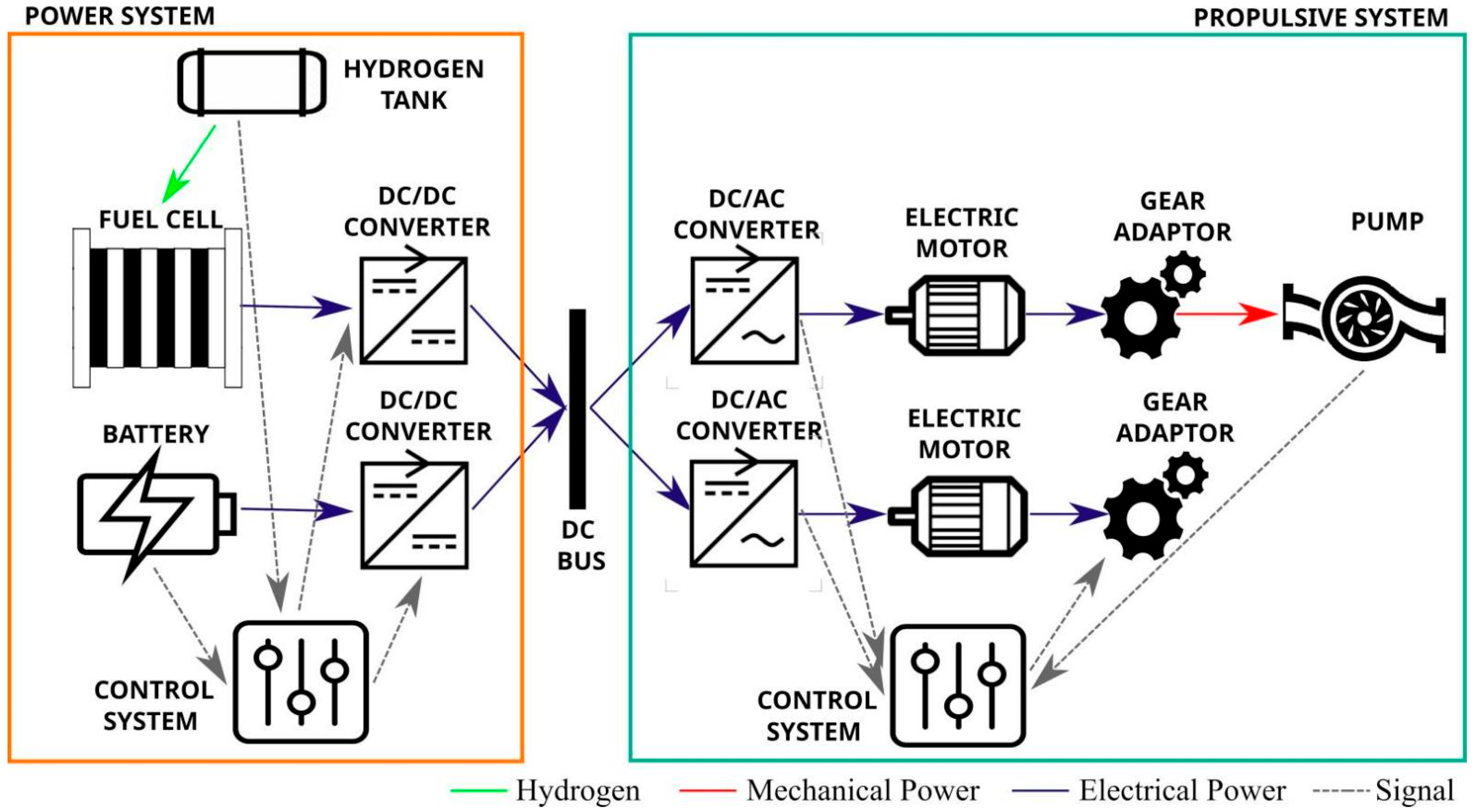
Considering these features, useful for calculating power consumption, the introduction of a fuel-cell system is evaluated, working together with the battery, with the aim of extending the vehicle’s range. The conceptual scheme of this new layout is illustrated in Figure 1. As shown, the main components can be gathered into two macro-systems:
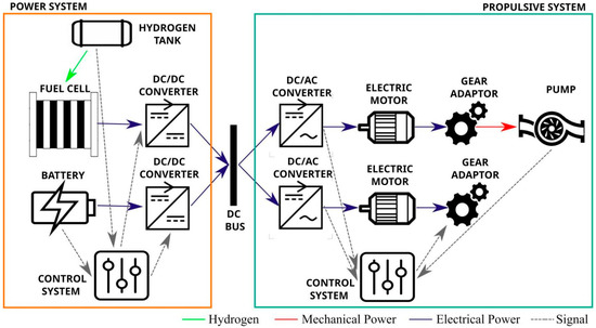
Figure 1.
Simplified scheme of the AMV innovative powertrain.
- The power system, which provides power and energy demands of the AMV, is useful for defining a specific power-sharing, and is composed of a fuel cell, battery, DC/DC converter, and power-sharing control systems;
- The propulsive system, that transforms the power system outputs into parameters useful for the AMV traction, is constituted by two BLDC motors, the propulsive and azimuth ones, formed by an electric motor, an inverter, and a motor control subsystem.
2.2. Power System
Electrochemically, fuel cells convert reactant chemical energy directly into electrical energy [17,20]. An external storage system continuously supplies reagents, unlike batteries. The fuel cell system and its auxiliary systems can be sized to meet the required operation’s energy needs, while the external hydrogen storage system is sized to meet the fuel cell system’s energy needs for the same mission. Since the energy density of the hydrogen storage system is much higher than that of batteries, fuel cell systems’ energy density can potentially exceed the batteries’ energy density.
Among the various types of fuel cells [26,27,28,29], low-temperature proton exchange membrane fuel cells (PEMFCs) are best suited for use in power generation systems aboard an ASV or AUV for the following reasons:
- the thermal energy requirements of an ASV and an AUV are minimal and strictly necessary to prevent the vehicle temperature from dropping below the minimum recommended value for the proper functioning of the on-board instrumentation;
- their weight must be as low as possible to maintain good vehicle handling;
- the compatibility of the devices with the marine environment, in which they operate, must be guaranteed;
- PEMFCs are the most mature from a technical and commercial point of view among the different types of low-temperature fuel cells.
The fuel cell power generation system with fuel cells and battery and without super-capacitors is the best configuration for the ASV propulsion system since the power demands of the considered ASV vehicle do not have a power peak request of such an extent as to justify the use of super-capacitors, which would unnecessarily burden the same vehicles.
The AMV Power System consists of a power-controlled PEM fuel cell subsystem, a Li-ion battery subsystem, and a metal hydride hydrogen storage subsystem. The PEM fuel cell power system is designed to be controlled by the powertrain control system and integrates an innovative and more efficient PEM stack. The powertrain system is complemented by an innovative low-pressure metal hydride hydrogen storage system, which is more compact than a conventional tank at the same pressure, and the Li-ion battery subsystem. The DC−DC converter models of the PEM fuel cell subsystem and the Li-ion battery subsystem have been simplified to reduce software calculation time.
The power system consists of three different blocks: the power-controlled PEM fuel cell power subsystem, the Li-ion battery subsystem, and the metal hydride hydrogen storage subsystem. After the implementation of each subsystem, their validation tests will be performed.
2.2.1. Power-Controlled PEM Fuel Cells Subsystem
The power-controlled PEM Fuel Cell subsystem consists of the PEM stack with all its ancillaries (measuring instruments, actuators, air blower, etc.), the DC−DC converter, and the control subsystem.
The main equations of the PEM Fuel Cells stack are Equations (1)–(6):
Equation (1) is the equation for the calculation of the real voltage of the PEM fuel cell stack, Equation (2) represents the current balance equation at the circuit main nodes, Equations (3) and (4) are the current equations for the capacitive anodic and cathodic activation phenomena, while Equations (5) and (6) are the voltage equations for the anodic and cathodic ohmic phenomena.
The main equations of the simplified DC−DC converter are Equations (7) and (8):
In Equations (7) and (8), and are respectively the DC−DC converter efficiency and the DC−DC converter duty ratio.
The equations for the electric loads of ancillaries and user, which are assumed as pure resistive loads, are Equations (9) and (10):
Equations (9) and (10) represent the currents and power balance equations for the PEM fuel cells subsystem.
The control subsystem regulates the DC−DC converter duty ratio, , which influences electrochemical phenomena (associated with parameters such as , , , , ), in a way that the electric power delivered by the power subsystem is equal to the electric power required by the control system of the entire hybrid electric propulsion system.
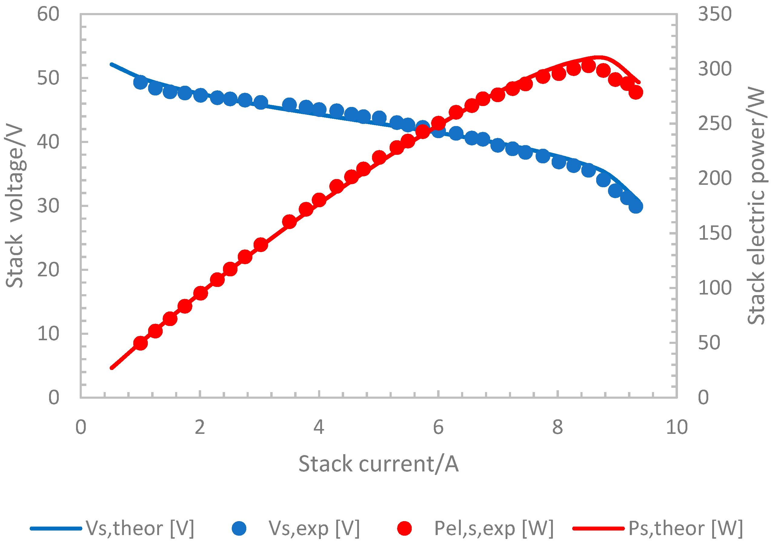
Regarding the validtion, the PEM stack simulated is the PEM stack model H300 type C, produced and marketed by the company H2Planet by Hydro2Power s.r.l., whose main technical data are reported in Table 1.

Table 1.
Main PEM stack technical data.
Figure 2 shows the comparison between the PEM stack experimental data supplied by the manufacturer and the polarization and electric power curves produced by the simulation model. Figure 2 shows that there is a good agreement between the simulation model results and the experimental data.
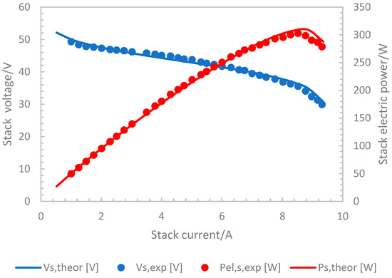
Figure 2.
Comparison between the PEM stack theoretical polarization (blue line) and electric power (red line) curves and PEM stack experimental data supplied by the manufacturer.
2.2.2. Li-Ion Battery Subsystem
The Li-ion battery subsystem consists of the Li-ion battery pack and the simplified DC−DC converter subsystem for the management of the charging and discharging phases.
In the discharging (
) and charging phases (
), the main equations of the Li-ion battery pack model are Equations (11) and (12) [30,31,32]:
In Equations (11) and (12) , , , , , , , , and are respectively the voltage, the current, the internal resistance, the constant voltage, the polarization constant or the polarization resistance, the low frequency filtered current, the extracted capacity, the capacity, the exponential voltage, and the exponential zone time constant.
The voltage of the battery pack at a fully charged state is calculated by adopting Equation (13) [30,31,32]:
The battery pack voltage at the exponential section and at the nominal zone are calculated by Equations (14) and (15) [30,31,32]:
In Equations (14) and (15),
and are the exponential and nominal capacities.
The equivalent circuit of the Li-ion battery pack is discussed somewhere else [28,29,30]. The parameters of the equivalent circuit can be modified to represent the Li-ion battery, based on its discharge characteristics (exponential voltage drop, normal discharge, and total discharge sections). The Simulink battery block implements a Li-ion battery pack dynamic model parameterized to represent the Li-ion battery pack installed on board the autonomous marine vehicle.
The model uses the SOC as a state variable [33], and the open circuit voltage is calculated using a nonlinear equation based on the analysis of the state of charge.
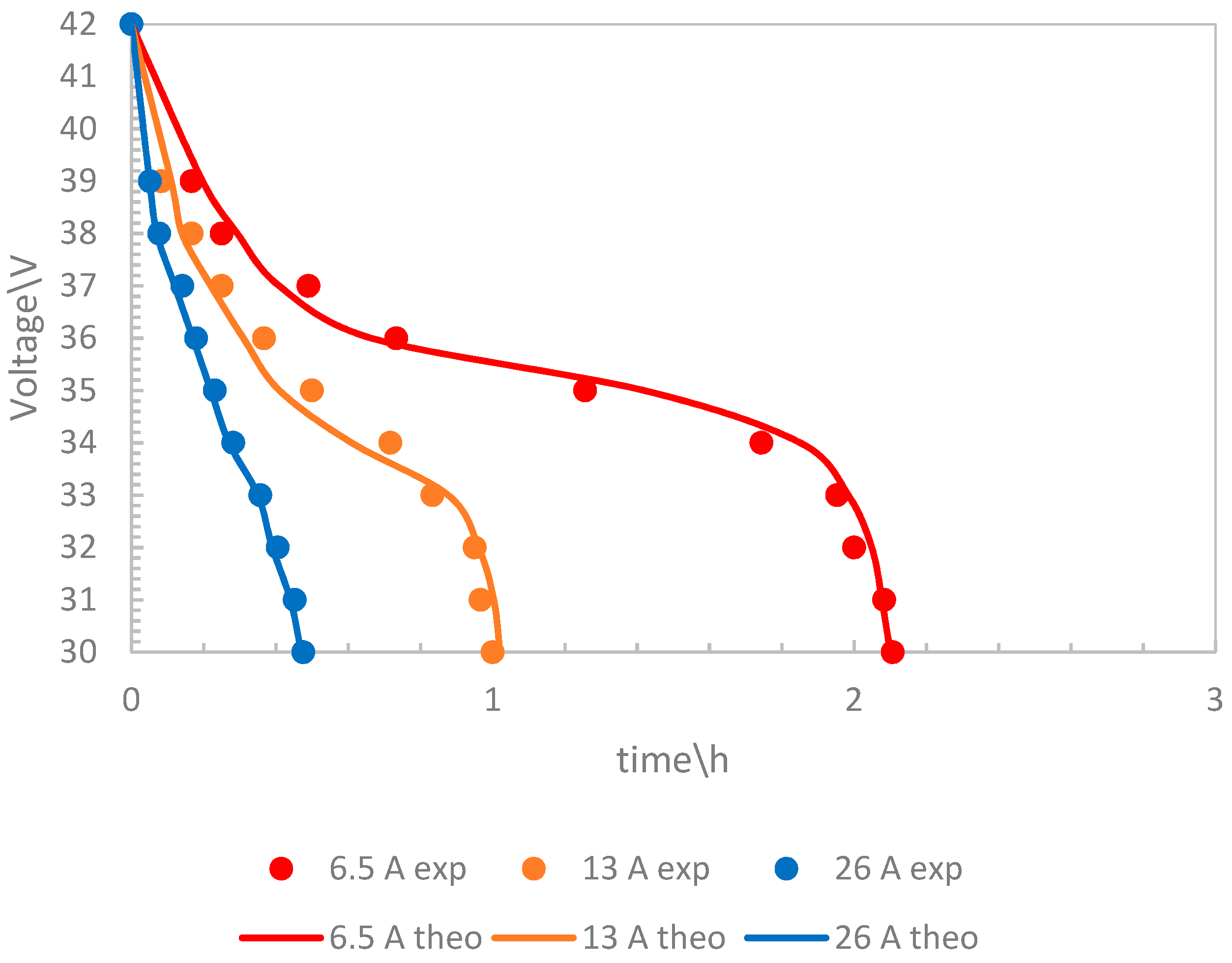
Regarding the battery validation, the Lithium-ion battery (NCM) pack simulated is the model IS36V13, which is produced by the company Map batteries by FAM batteries, and it has a nominal voltage and capacity equal to 37 V and 13 Ah. All other technical specifications can be found in [34].
Figure 3 shows the comparison between the Li-ion battery pack experimental data supplied by the manufacturer and the Li-ion battery pack battery theoretical discharge curve produced by the simulation model at different typical operating discharge currents (6.5, 13, 26 A). Figure 3 shows that there is a good agreement between the simulation model results and the experimental data.
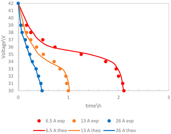
Figure 3.
Comparison between the theoretical Li-ion battery pack discharge theoretical (theo) curves and the Li-ion battery pack experimental (exp) data, supplied by the manufacturer at different typical operating currents (6.5, 13, and 26 A).
The amount of energy available and accumulated instant by instant are functions of the battery SOC. Improving the available capacity has been necessary to carefully assess the depth of discharge, the charging voltage, and the currents in the processes of charging and discharging [35].
2.2.3. Metal Hydride Hydrogen Storage Subsystem
The hydrogen storage system based on metal hydrides (MH) operates in discharging mode, and the main equation of the hydrogen storage system is Equation (16):
where , , , , and are, respectively, the instantaneous and maximum hydrogen moles in the storage system, the state of charge at the initial instant , the number of fuel cells, the instantaneous stack current, and the conversion parameter for the calculation of the state of charge variation from the stack charge variation.
The MH H2 storage system simulated is the My-H2 900, produced and marketed by the company H2Planet by Hydro2Power s.r.l., whose main technical data are reported in Table 2.
Table 2.
Main MH-H2 tank technical data.
The PCT diagram of the metal hydride shows the equilibrium relationship between the hydrogen pressure and the percentage of hydrogen mass, %m,H2, as a function of the amount of alloy present in the system. Under dynamic conditions, i.e., during charging or discharging, the respective curve deviates from this equilibrium curve to a greater or lesser extent, depending on the cooling/heating parameters chosen, in particular the temperature.
Figure 4 shows the comparison between the theoretical desorption curve MH PCT and the experimental data from MH provided by the manufacturer at the typical operating temperature (20 °C). Figure 4 shows that there is good agreement between the results of the simulation model and the experimental data.
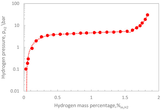
Figure 4.
Comparison between the theoretical Metal Hydride PCT desorption curve and experimental data, supplied by the manufacturer at the typical operating temperature (20 °C).
2.2.4. Power System Control Strategy
Control strategies are fundamental to allow a proper management of the energy sources within the powertrains [36,37]. Between the numerous strategies, the state machine control strategy is based on different states useful for selecting the operating power level of the Fuel Cell (FC) subsystem [38]. This control technique aims to reduce the FC power fluctuations to improve efficiency and lifetime. For this reason, the fuel cell power fluctuations occur only when the battery state of charge (SOC) exceeds the predetermined thresholds.
In general, the control technique tries to keep the fuel cell in the optimal state, i.e., the value corresponding to the maximum efficiency, which is its only output parameter. Nevertheless, the only controlled parameter, the fuel cell power, is changed according to the battery SOC between the maximum power output and the minimum value. Therefore, the fuel cell is never turned off to avoid the long turn-on times and low efficiency at low power rates. Two input parameters are considered, namely the battery SOC and the fuel cell subsystem power at the previous time step. The battery operates in a wide SOC range between 20% and 100%, which is set as the operating limit, but four intermediate levels of SOC are considered, namely 30%, 40%, 80%, and 90%, which are useful for appropriate charging or discharging operations. Finally, to ensure the proper behavior of the fuel cell subsystem under the extreme conditions of the battery subsystem, the performance of the fuel cell at the previous time is studied, considering two threshold values, namely the maximum and minimum performance of the fuel cell. The limited values of the input and output parameters are summarized in Table 3.
Table 3.
Limits imposed on input and output parameters of the state machine control.
Evaluating the suitable combinations of the input limits, six states are considered, listed in Table 4.
Table 4.
Control rules of the state machine control.
Following these rules, the control strategy is composed of a hysteresis cycle for each SOC extreme condition, as shown in Figure 5: in detail, a hysteresis cycle between 20% and 40% of battery SOC is implemented (Figure 5a), while another one between 80% and 100% of battery SOC (Figure 5b).
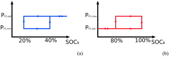
Figure 5.
Hysteresis cycle of the state machine control system: (a) low battery SOC levels; (b) high battery SOC levels.
A further feature implemented in the power-sharing strategy concerns the simulation stops; when one of the two SOCs reaches the minimum value allowed (11% for the SOCH2 and 20% for the SOCB), the vehicle is stopped and the drive cycle is not completed.
2.3. Propulsive System
The propulsive system of the tested AMV consists of two brushless DC (BLDC) motors, which are named motor system, for each propulsive pump; during the test, 2 or 4 propulsive pumps are used. The BLDC motors used are three-phase synchronous motors with permanent magnets on the rotor and electronic commutators instead of brush gears and mechanical commutators. In this way, the system takes advantage of three-phase motors, behaves like a DC system, and avoids limitations of electromagnetic interference, frame, speed, and noise [39]. Compared to brushed DC and induction motors, they offer satisfactory performances such as high efficiency, long life, noiseless operation, wide speed ranges, high torque relative to frame size, excellent dynamic behavior, and good speed–torque characteristics.
Generally, BLDC systems consist of three different blocks: the electric motor, the inverter, and the control system. After implementation, the validation tests are performed.
2.3.1. Electric Motor
Brushless DC motors are synchronous motors, namely the two magnetic fields, belonging to the stator and rotor, have the same frequency. They can be single-phase, two-phase, and three-phase, according to the stator windings. Generally, three-phase motors are the most used, thanks to their high efficiency and accurate control. In this case, permanent magnets’ synchronous motors with trapezoidal back electromotive force, rather than sinusoidal ones, are the most used in BLDC systems [40]. The model implemented is based on the block present in the Matlab/Simulink environment [41,42]. The main assumption made is the linear magnetic circuit, without stator and rotor saturation.
The electric motor behavior is described by Equations (17)–(19), which are useful for calculating the three-phase currents (ia, ib, and ic), considering the phase voltages (Vab and Vbc), the flux amplitude induced by the rotor magnet to the stator (λ), and the electromotive forces in per-unit (φa, φb, φc):
2.3.2. Inverter
The inverter is fundamental in BLDC systems. It is needed to convert the single-phase direct current supplied by the power grid into the three-phase alternating current. In addition, it is critical for detailed control of the electric motor by determining the required mechanical torque and speed of the motor. The detailed modeling of the inverter, which consists of six switches, requires a high computational effort that is suitable for simulating a detailed behavior of the device but for a limited simulation time. However, the scope of this work is to analyze an autonomous marine vehicle in different simulation campaigns, and a simplified model is more appropriate in terms of low computational cost and sufficient in terms of data accuracy.
The inverter model used is based on the block available in the Matlab Simulink environment [42,43]. It consists of a DC-controlled current source, whose behavior is described in Equation (20), and two AC-controlled voltage sources that manage the trapezoidal inputs provided by the electric motor model:
The AC reference currents, calculated through the control system, the back electromotive force voltage, and the current are the inputs needed to compute the inverter voltages. The main assumption is the rate limiter, which regulates the output voltage during transitions, employing a saturation degree coefficient.
2.3.3. Motor Control Strategy
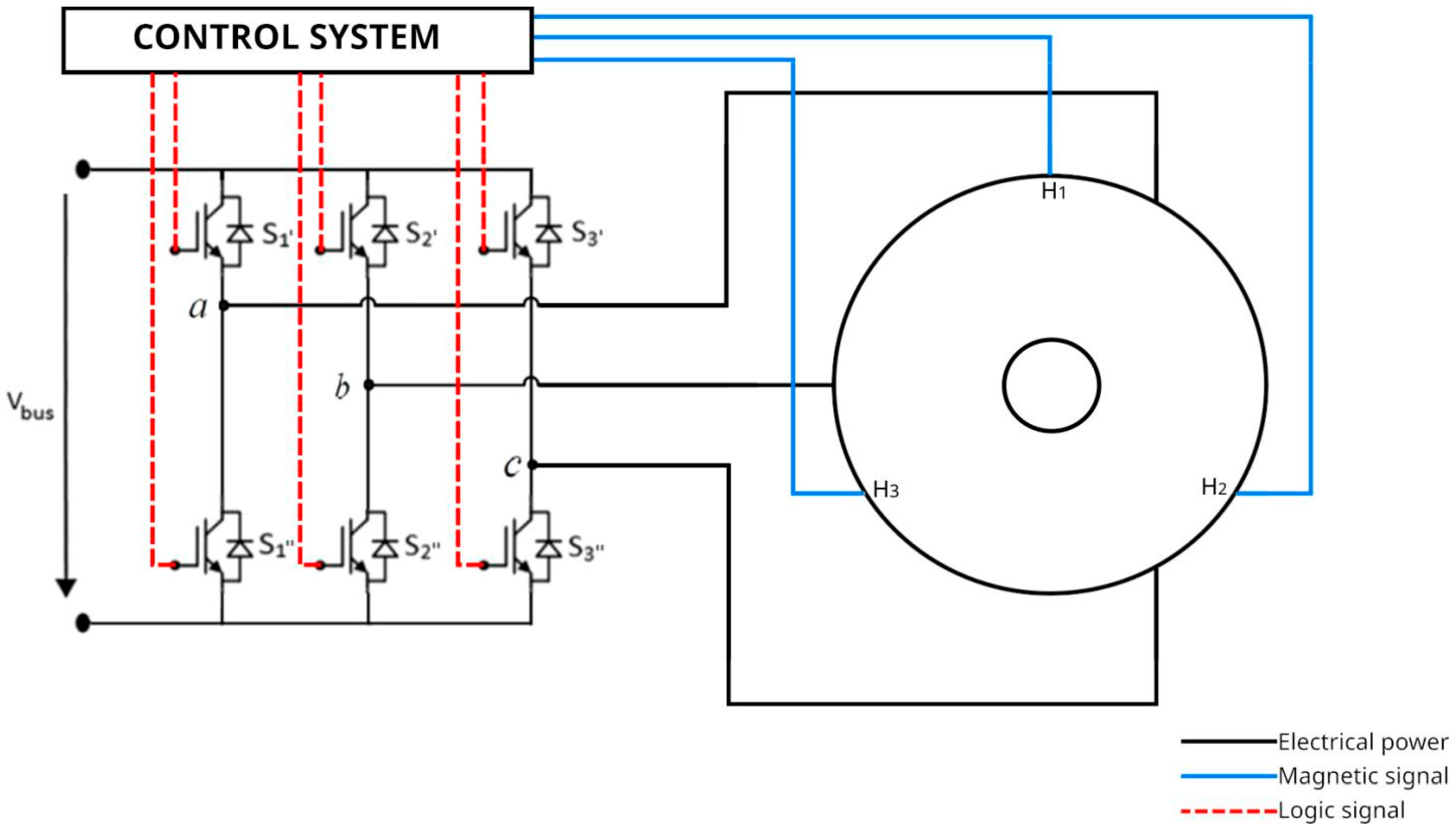
Once the main components of the BLDC motor have been defined, it is important to analyze the electronic commutations, capable of controlling the interaction between the inverter and electric motor and achieving the outputs needed, as shown in Figure 6.

Figure 6.
Motor system: electric motor, inverter, and control subsystems.
In the present work, among the different commutation strategies, the communication with Hall sensors is performed, given by the BLDC motor used [44,45]. In brief, there are three Hall sensors (H1, H2, and H3 in Figure 6) on the motor at an angle of 120°, which detect the magnetic field of the control magnet on the shaft. In this way, the signal received, as the combination of the Hall sensors, is univocal for each 60° of rotation. Therefore, according to the rotor position and the outputs needed, it is possible to change the stator magnetic field, acting on the three-phase voltages and, hence, on the duty-cycle of the inverter switches (S1′, S1″, S2′, S2″, S3′, S3″).
The control strategy can be divided into two subsystems, namely a commutation system and a speed controller system. The former is a rule-based strategy, capable of providing a vector that contains phase voltage details, starting from the hall sensor signals. For example, a rule is shown in the following sentence:
“If Hall sensor signal is [1 0 1] then phase voltage vector is [+1 −1 0]”
The speed controller is useful for calculating the torque reference value, namely the torque imposed to perform a specific journey. A proportional-integral (PI) structure is used, considering as a controlled value the error between the reference and real values of the motor rpm.
By combining the outputs of the two subsystems with a suitable motor factor, a control vector can be created that specifies a suitable duty cycle for each inverter switch.
2.3.4. Validation
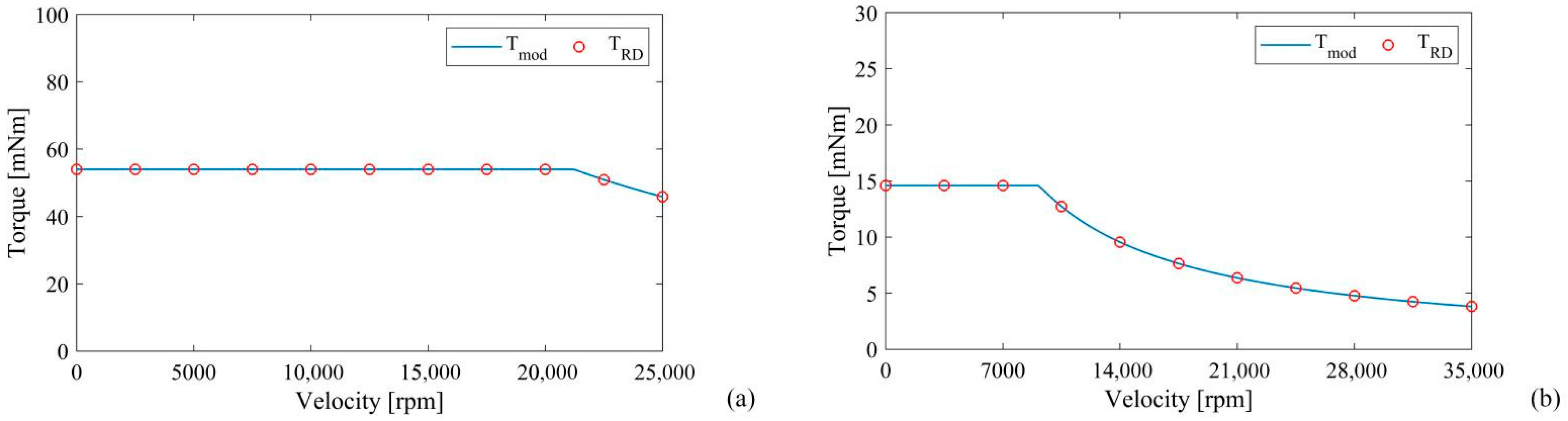
As shown in the simplified schematic of the AMV in Figure 1, the propulsion system consists of two brushless DC motors, one for propulsion and one for directional control, the azimuth motor. Due to these tasks, two motors with different characteristics are tested in the numerical simulations, which are listed in Table 5. Both are connected to the DC bus and work together depending on the requirements of the vehicle. The drive motor is a Maxon Ec-4pole, a motor with a rated speed of 16,800 rpm and a rated torque of 54 mNm, coupled with a 14:1 reduction gearbox [46]. The azimuth motor, on the other hand, is a Faulhaber 2232-BX, characterized by a rated speed of 4930 rpm and a rated torque of 14.3 mNm, with a reduction ratio of 59:1 [47].
Table 5.
Performance features of the two electric motors.
Starting from these values, and considering the torque trends present on the data sheets provided by the manufacturing company, validation tests have been performed, obtaining as results the plots shown in Figure 7; the blue line represents the model behavior, while the red dots are the real motor data. The error achieved during the simulations is less than 1%; therefore, the model turns out to be appropriate for the studied application.
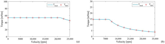
Figure 7.
Validation tests of (a) the propulsion motor and (b) the directional motor.
3. Simulation and Results
The hydrogen-based marine vehicle was numerically tested in four case studies to evaluate the performance and range of the vehicle and to discuss the SOC of the fuel cell and battery. The energy parameters of each drive cycle are presented, and the response of the powertrain is mentioned.
3.1. Case Studies
In the simulation campaigns, four journeys with different power levels and time intervals are considered, which are useful to test the AMV under different conditions. Figure 8 shows the power and energy requirements in blue and red, respectively, measured at the DC bus connecting the power and motor systems. They are the sum of the motor demand, i.e., the electrical power requested by the propulsion and azimuth motors, and the auxiliary power, i.e., the theoretical consumption of the instruments on board.
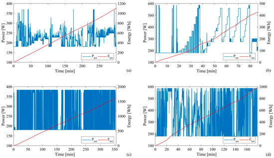
Figure 8.
Power (blue line) and energy (red line) trends of the four analyzed journeys: (a) Journey 1; (b) Journey 2; (c) Journey 3; (d) Journey 4.
As shown in the figure, all trips have a minimum power of 176 W, which is the instrument consumption considered as a constant power for the whole drive-cycle time.
In Figure 8a, the power and energy demands of Journey 1 are shown. The trip lasts 5 h and has numerous power fluctuations, with a maximum value of 370 W and an energy consumption of 1100 Wh. The second drive cycle, shown in Figure 8b, achieves higher power but lower energy consumption compared to Journey 1, about 585 W and 425 Wh, respectively, due to less frequent power fluctuations and a shorter drive time of 85 min. Journey 3 (Figure 8c), unlike the other case studies, uses only two propulsive pumps, instead of four, namely, two motor systems (composed of an azimuth and a propulsive motor) are used. Consequently, the maximum power value is 385 W, with very frequent and faster power fluctuations, more than the other journeys. Although the power range is limited, the energy consumption of Journey 3 is the highest, about 1615 Wh, since the trip is about 6 h long. Finally, Journey 4 (Figure 8d) is almost 3 h long, with high power, 585 W, the same value as Journey 2, but the total energy is less than 1 kWh, a value lower than that of Journey 3.
3.2. Result Analysis
The four drive-cycles shown in Figure 8 are used to numerically test the autonomous marine vehicle and analyze the behavior of the powertrain under different operating conditions without changing the size of the energy storage device. The energy consumed by the fuel cell and the battery varies greatly depending on the trip tested; therefore, the final values of the hydrogen SOC and the battery SOC are different. A separate section is dedicated to each journey.
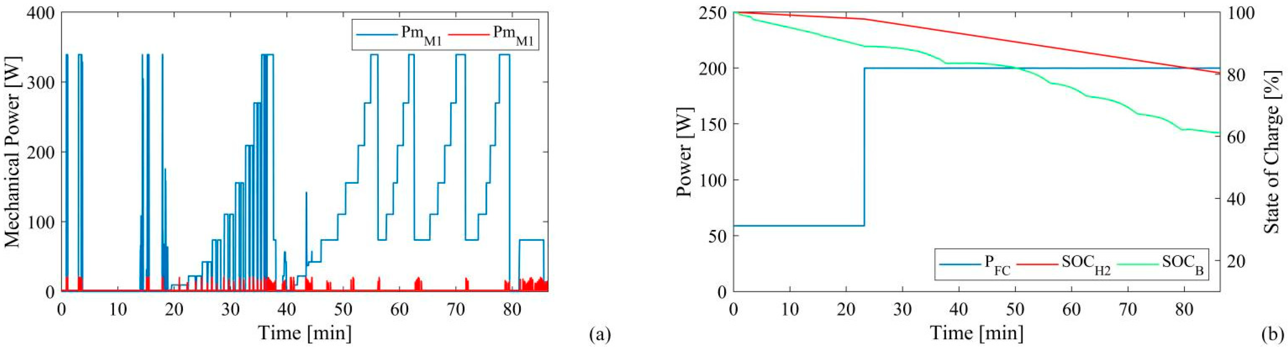
3.2.1. Journey 1
The first Journey is almost 5 h long, with a smaller power interval compared to the other journeys, between 176 W and 370 W, even though four motor systems are used. The simulation results are shown in Figure 9. The right part (Figure 9a) shows the mechanical power variations of the propulsion motor and the azimuth motor, while the left part (Figure 9b) illustrates the power system performances, namely the fuel cell power, the hydrogen SOC and the battery SOC. The power of the propulsion motor (blue line in Figure 9a) exhibits numerous and sudden fluctuations between 0 W and 160 W, while the azimuth motor is turned on a few times during the trip, and its power (red line in Figure 9a) assumes an impulse trend in a range between 2 W and 20 W. As in the other runs, the fuel cell power (blue line on the left axis in Figure 9b) exhibits a step-like trend starting from the minimum power (60 W) as the battery is fully charged and varying to the optimal value (about 200 W) when one of the control strategy thresholds is exceeded. The maximum FC power value is not reached as the battery SOC remains at a high level. This power results in a wide range of hydrogen SOC (red line on the right axis in Figure 9b) arriving at 21% and consuming about 64 g of hydrogen; in contrast, the battery SOC (green line on the right axis in Figure 9b) starts at 100% and arrives at 70%. During this drive, the fuel cell delivers a larger fraction of energy, about 965 Wh, than the battery due to the smallest power fluctuations compared to the other drive cycles. In other words, the fuel cell works as a prime mover, covering the energy demand and operating quasi-steady-state conditions, while the battery covers the power peaks when the energy demand is high and is charged by the fuel cell when the energy demand is low.
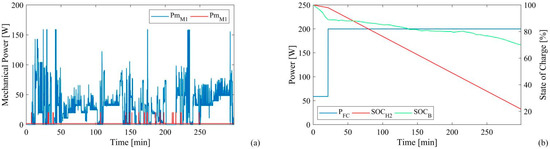
Figure 9.
AMV performance in Journey 1: (a) Motor mechanical power trends; (b) Fuel cell power, hydrogen tank and battery state of charge trends.
3.2.2. Journey 2
The second Journey is the shortest among the four drive-cycles, being more or less a quarter compared to Journey 3, around 85 min, and also the one with the lowest energy demand, consuming about 425 Wh, which is also almost a quarter of the energy required for the Journey 3.
The performance of the AMV in Journey 2 is shown in Figure 10. Given the low value of the required energy, the vehicle can complete the journey with satisfactory performance. The mechanical power of the two motors follows the trend of the energy demand, excluding the consumption by the auxiliary and measurement systems. The power of the propulsion motor (blue line in Figure 10a) varies in a wide interval between 0 W and 340 W, while the power of the azimuth motor (red line), which is characterized by a sequence of numerous impulses, has 20 W as the maximum mechanical power.
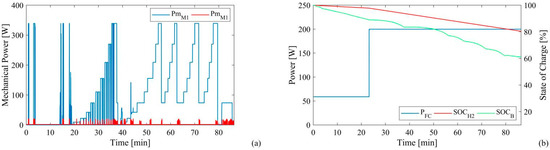
Figure 10.
AMV performance in Journey 2: (a) Motor mechanical power trends; (b) Fuel cell power, hydrogen tank and battery state of charge trends.
As for the power system performance, the power of FC goes from the minimum value to the optimal value after 25 min and remains the same until the end of the cycle. According to this trend, the hydrogen SOC reaches a value of 80% at the end of the cycle, with a hydrogen consumption of 16 g. On the other hand, the battery SOC is very variable, with successive charging and discharging phases; the final value is about 61%, and, consequently, the energy provided by the battery is about 195 Wh.
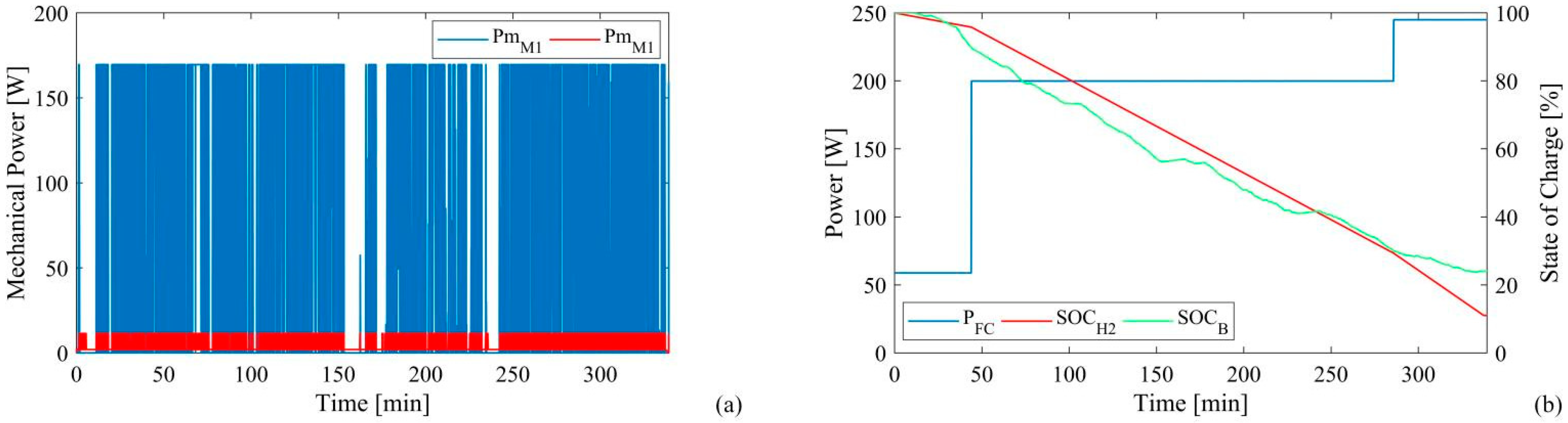
3.2.3. Journey 3
The third Journey is the most critical because it takes the longest, about 6 h, and has the highest energy consumption, about 1.6 kWh, compared to the four drive-cycles tested. It is the only Journey where two motors are used. As shown in Figure 11a, the mechanical power of the drive motors reaches a maximum value of 170 W. The power of the azimuth motor, on the other hand, follows the same trend as that of the propulsion motor, with a narrow interval between 2 W and 12 W. Although the power interval is not very large, the long travel time results in huge energy consumption that the drive system cannot provide. The AMV stops driving after 340 min because the fuel cell reaches the imposed limits for the hydrogen SOC (11%), as shown in Figure 11b, and consequently, the power-sharing strategy aborts the simulations. As for the fuel cell performance, it adopts the three fixed rates given by the wide interval of the battery SOC. In fact, the trend of the battery SOC is oscillating due to the numerous charging and discharging phases and its minimum value is 24%, reached at the end of the Journey.

Figure 11.
AMV performance in Journey 3: (a) Motor mechanical power trends; (b) Fuel cell power, hydrogen tank and battery state of charge trends.
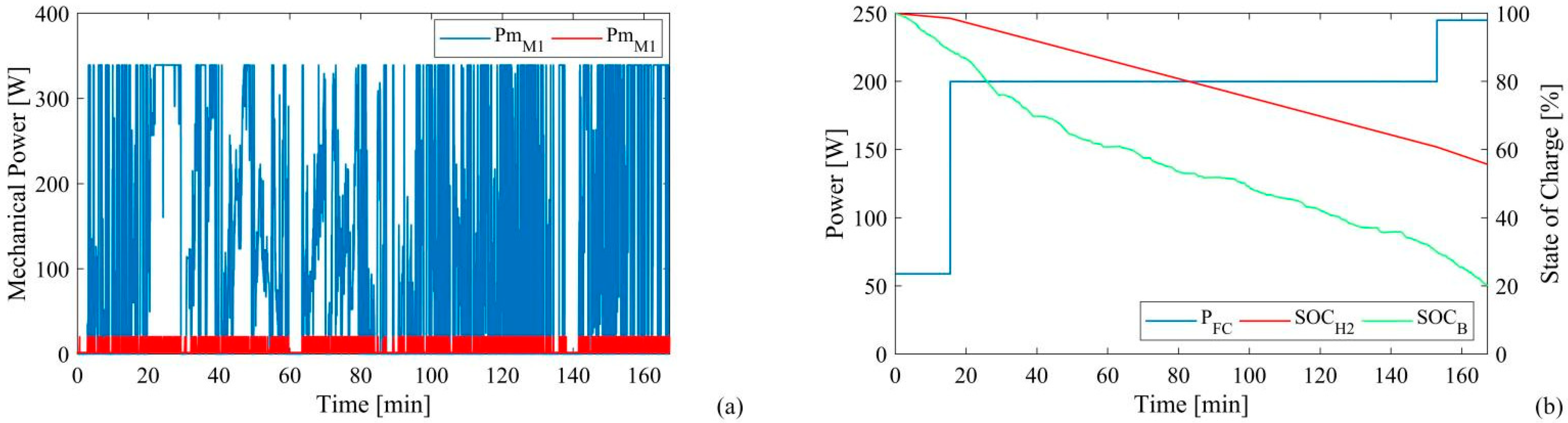
3.2.4. Journey 4
The last Journey shows medium values compared to the other cycles, with an energy consumption of 980 Wh. As in the first two cycles, the energy stored on board is sufficient to complete the drive cycle, but a correction of the control system is required for the AMV to complete the journey. In fact, Figure 12 shows the performance of the AMV without corrections and testifies that one of the two SOC limits is reached. This is due to the characteristics of the control strategy and the large difference between the two SOCs; in other words, the hydrogen SOC is much higher than the battery SOC at all times, and the limit conditions are easily reached. Although the hydrogen SOC remains at 55%, the battery SOC reaches the lower limit of 20%, causing the simulation to terminate. The main reason for this behavior is related to the journey features, namely the pronounced and contiguous power variations between 176 W and 585 W. Therefore, the battery cannot deliver the energy variations of the journey if the fuel cell maintains the optimal power output between 80% and 30% of the trend of the battery SOC.
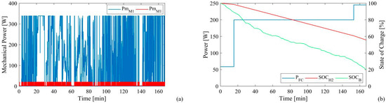
Figure 12.
AMV performance in Journey 4, without control system correction: (a) Motor mechanical power trends; (b) Fuel cell power, hydrogen tank and battery state of charge trends.
To address this issue, the SOCL and SOCML values of the control strategy are changed from 30% and 40% to 50% and 60% for Journey 4 only. The updated performance with the adjusted control strategy is shown in Figure 13. The propulsion motor reaches high values, as in Journey 2 and more than the other Journeys, fluctuating in an interval between 0 W and 340 W; its trend shows sudden fluctuations, as in Journey 3. The azimuth motor, on the other hand, since four motors are active, fluctuating in the standard range between 2 W and 20 W; it follows the operating conditions of the propulsion motor and assumes its maximum power when the propulsion motor is on. Figure 13b illustrates the power system performance. As with Journey 3, unlike the other journeys, the fuel cell power assumes all three values specified by the power-sharing strategy, even if its energy demand falls in between. The maximum fuel cell power (250 W) is required from about 100 min, about halfway through the trip, until the end. Under these circumstances, the hydrogen SOC has a final value of 47%, eight points less than in the case without adjustments to the control strategy, requiring 43 g of hydrogen. At the same time, the battery SOC is at 25% at the end of the journey, which means that the lowest threshold of the control system is not exceeded, and the journey can be ended.
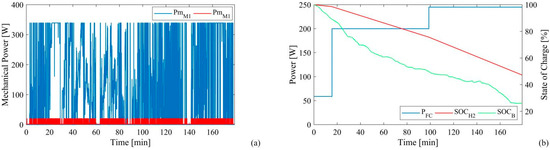
Figure 13.
AMV performance in Journey 4, with control system correction: (a) Motor mechanical power trends; (b) Fuel cell power, hydrogen tank and battery state of charge trends.
3.2.5. Summary Considerations
In the result analysis, the AMV powertrain model has been numerically tested on four journeys, with different time intervals, power, and energy demands (shown in Table 6), and its performance is summarized in Table 7. During the first Journey, the motor system mechanical power assumes a maximum value of 180 W with variable trends; the hydrogen consumption is approximately 64 g, given by the fuel cell energy consumption (1 kWh) while the battery provides a moderate energy amount, remaining with a final SOC value of 70%. On the contrary, Journey 2 requires a maximum motor power of approximately 360 W; being the journey with the lowest energy demand than the other ones, the hydrogen consumption is only 16 g, but the battery provides almost 195 Wh, reaching a minimum SOC value of 61%. The third Journey instead requires a higher energy amount, about 1.60 kWh, more than the one needed in the other cycles; nevertheless, the maximum mechanical motor system power is only 180 W. The energy stored on board, as the hydrogen in the tank and the battery capacity, is not enough to complete the journey, stopping at 340 min (96% of the journey). The fuel cell supplies about 1087 Wh, consuming the whole hydrogen amount usable, while the remaining energy part is provided by the battery, about 375 Wh. In the end, the last Journey requires 980 Wh, with the same level of maximum motor power for Journey 2. Owing to the high and consecutive power variations, a modified control strategy is required to complete the journey. With these new features, the powertrain completely fulfills the vehicle demands; the fuel cell provides 632 Wh, consuming 43 g of hydrogen, while the battery supplies 368 Wh, concluding the journey with an SOC level of 25%.
Table 6.
Performance features of the four analyzed journeys.
Table 7.
AMV achieved performance in the four analyzed journeys.
4. Conclusions
This paper presents an innovative fuel cell hybrid powertrain for an autonomous marine vehicle, whose performance is analyzed using multiphysics and dynamic numerical modeling of the main vehicle components, namely fuel cell, battery, inverter, electric motors, and control systems.
The implemented model was tested to simulate the fuel cell hybrid powertrain in four journeys, with different characteristics to evaluate the performance and range of the vehicle and to discuss the SOC of the fuel cell and battery. In the tests, hydrogen consumption varied from 16 g for Journey 2 to 71 g for Journey 3, which is closely related to the energy delivered by the fuel cell. However, each component exhibited different peculiarities in the four journeys discussed. For example, Journey 3 required a higher amount of energy, about 1.60 kWh, than the other journeys. Nevertheless, the maximum motor power was only 210 W because only 2 of 4 motors were on during the journey. The energy stored on board was not enough to complete the trip. The trip was stopped after 340 min (96% of the cycle). The fuel cell supplied about 1087 Wh, consuming all of the hydrogen stored on board (about 71 g), while the remaining energy portion (about 375 Wh) was supplied by the battery, which completed the trip at 25% SOC.
Journey 4, on the other hand, requires an intermediate amount of energy (980 Wh) with a maximum mechanical motor power of 360 W. Due to the significant and continuous power fluctuations between 176 W and 585 W, the journey could not be completed with the implemented simplified control system. Therefore, a modified control strategy was implemented in which the thresholds were changed to terminate the run. With these new features, the powertrain fully met the requirements of the vehicle; the fuel cell delivered 632 Wh and consumed 43 g of hydrogen, while the battery delivered 368 Wh and completed the trip with an SOC level of 25%.
Given these limitations, further work could consider evaluating new control systems capable of increasing the vehicle’s range by exploiting the characteristics of the propulsion system.
In other words, in this paper:
- A fuel cell hybrid powertrain for an autonomous marine vehicle was developed by means of dynamic and multi-physics relations;
- Four journeys were considered to test the innovative vehicle on different conditions;
- The main parameter of the powertrain, concerning power, consumption and SOC were monitored by means of a control system ad-hoc implemented;
- The feasibility of each work journeys was verified, highlighting criticality.
The application tested proves that the use of hydrogen in marine applications can improve the performance of the electric powertrain and increase the range of the vehicle with less environmental impact compared to battery-based powertrains. The energy transition requires radical choices in all sectors, especially in the mobility sector, which produces a substantial amount of emissions. In this scenario, hydrogen-based solutions could be an important support, also in maritime applications, guaranteeing zero emissions in seawater.
Author Contributions
Conceptualization, G.D.L., F.P., F.L., G.T., V.B., N.P., M.C. and P.F.; Data curation, G.D.L., F.P. and P.F.; Formal analysis, G.D.L., F.P. and P.F.; Investigation, G.D.L., F.P. and P.F.; Methodology, G.D.L., F.P. and P.F.; Project administration, F.L., M.C. and P.F.; Resources, G.T., V.B., N.P. and M.C.; Software, G.D.L. and F.P.; Supervision, P.F.; Validation, G.D.L., F.P. and P.F.; Visualization, F.P. and P.F.; Writing—original draft, G.D.L., F.P. and P.F.; Writing—review and editing, G.D.L., F.P. and P.F. All authors have read and agreed to the published version of the manuscript.
Funding
This research received no external funding.
Institutional Review Board Statement
Not applicable.
Informed Consent Statement
Not applicable.
Acknowledgments
The authors gratefully acknowledge the Italian Ministry of University and Research for the financial support to Project No. ARS01 00682 ARES—Autonomous Robotics for the Extended Ship—CUP H56C18000160005, under the Italian National Research Program PON “Ricerca e Innovazione” 2014–2020, Action II.2, Specialization area: “Blue Growth”.
Conflicts of Interest
The authors declare no conflict of interest.
Nomenclature
| Symbols | Parameter | Units |
| A | Exponential Voltage | V |
| B | Exponential zone time constant | A−1 h−1 |
| C | Capacity | Ah |
| C | Capacitance | F |
| D | Duty ratio | - |
| E | Constant Voltage | V |
| η | Efficiency | - |
| φ | Electromotive forces in per-unit | - |
| HHV | high heating value | J/kg |
| ı | Current | A |
| K | Polarization constant or polarization resistance | V A−1 h−1 or Ω |
| k | conversion parameter | C |
| L | Inductance | H |
| λ | Flux amplitude induced by the rotor magnets in the stator phases | V s |
| mol | moles | mol |
| n | number | - |
| OCV | Open Circuit Voltage | V |
| ω | Angular velocity | rad/s |
| P | Power | W |
| p | Number of pole pairs | - |
| R | Resistance | Ω |
| SOC | State of charge | - |
| t | time | s |
| V | Voltage | V |
| Subscripts | Parameter | |
| a | Phase a of the three-phase parameter | |
| AC | Alternative current | |
| an | anodes | |
| aux | referred to the ancillaries | |
| b | Phase b of the three-phase parameter | |
| B | Referred to the battery | |
| batt | battery | |
| c | Phase c of the three-phase parameter | |
| cat | cathodes | |
| el | electrolyte | |
| exp | exponential | |
| ext | extracted | |
| fc | Fuel cell | |
| full | fully charged state | |
| H | High level | |
| H2 | hydrogen | |
| in | At the inlet | |
| L | Low level | |
| loss | Owing to losses | |
| m | Motor | |
| max | Maximum level | |
| min | Minimum level | |
| ML | Medium-low level | |
| MH | Medium-high level | |
| nom | nominal | |
| opt | Optimum level | |
| out | At the outlet | |
| s | stack | |
| sw | Stator winding | |
| user | referred to the electric user | |
| 1 | referred to the resistive branch | |
| 2 | referred to the capacitive branch | |
| Superscripts | Parameter | |
| * | Low frequency filtered | |
References
- Yan, R.; Pang, S.; Sun, H.; Pang, Y. Development and Missions of Unmanned Surface Vehicle. J. Mar. Sci. Appl. 2010, 9, 451–457. [Google Scholar] [CrossRef]
- Naval Studies Board; National Research Council. Autonomous Vehicles in Support of Naval Operations; National Academies Press: Cambridge, MA, USA, 2005; ISBN 978-0-309-09676-8. [Google Scholar]
- Carlson, D.F.; Fürsterling, A.; Vesterled, L.; Skovby, M.; Pedersen, S.S.; Melvad, C.; Rysgaard, S. An Affordable and Portable Autonomous Surface Vehicle with Obstacle Avoidance for Coastal Ocean Monitoring. HardwareX 2019, 5, e00059. [Google Scholar] [CrossRef]
- Bauk, S.; Kapidani, N.; Lukšic, Ž.; Rodrigues, F.; Sousa, L. Autonomous Marine Vehicles in Sea Surveillance as One of the COMPASS2020 Project Concerns. J. Phys. Conf. Ser. 2019, 1357, 012045. [Google Scholar] [CrossRef]
- Thompson, F.; Guihen, D. Review of Mission Planning for Autonomous Marine Vehicle Fleets. J. Field Robot. 2019, 36, 333–354. [Google Scholar] [CrossRef]
- Benjamin, M.R.; Schmidt, H.; Newman, P.M.; Leonard, J.J. Nested Autonomy for Unmanned Marine Vehicles with MOOS-IvP. J. Field Robot. 2010, 27, 834–875. [Google Scholar] [CrossRef]
- Bruzzone, G.; Odetti, A.; Caccia, M.; Ferretti, R. Monitoring of Sea-Ice-Atmosphere Interface in the Proximity of Arctic Tidewater Glaciers: The Contribution of Marine Robotics. Remote Sens. 2020, 12, 1707. [Google Scholar] [CrossRef]
- Caccia, M.; Bibuli, M.; Bono, R.; Bruzzone, G.; Bruzzone, G.; Spirandelli, E. Unmanned Surface Vehicle for Coastal and Protected Waters Applications: The Charlie Project. Mar. Technol. Soc. J. 2007, 41, 62–71. [Google Scholar] [CrossRef]
- Odetti, A.; Bruzzone, G.; Altosole, M.; Viviani, M.; Caccia, M. SWAMP, an Autonomous Surface Vehicle Expressly Designed for Extremely Shallow Waters. Ocean. Eng. 2020, 216, 108205. [Google Scholar] [CrossRef]
- Bradley, T.H.; Moffitt, B.A.; Fuller, T.F.; Mavris, D.N.; Parekh, D.E. Comparison of Design Methods for Fuel-Cell-Powered Unmanned Aerial Vehicles. J. Aircr. 2009, 46, 1945–1956. [Google Scholar] [CrossRef]
- Thomas, J.P.; Qidwai, M.A.; Kellogg, J.C. Energy Scavenging for Small-Scale Unmanned Systems. J. Power Sources 2006, 159, 1494–1509. [Google Scholar] [CrossRef]
- Verstraete, D.; Lehmkuehler, K.; Wong, K.C. Design of a Fuel Cell Powered Blended Wing Body UAV; American Society of Mechanical Engineers Digital Collection: New York, NY, USA, 2013; pp. 621–629. [Google Scholar]
- Choi, S.; Wang, G. Advanced Lithium-Ion Batteries for Practical Applications: Technology, Development, and Future Perspectives. Adv. Mater. Technol. 2018, 3, 1700376. [Google Scholar] [CrossRef]
- Xia, S.; Wu, X.; Zhang, Z.; Cui, Y.; Liu, W. Practical Challenges and Future Perspectives of All-Solid-State Lithium-Metal Batteries. Chem 2019, 5, 753–785. [Google Scholar] [CrossRef]
- Sorlei, I.-S.; Bizon, N.; Thounthong, P.; Varlam, M.; Carcadea, E.; Culcer, M.; Iliescu, M.; Raceanu, M. Fuel Cell Electric Vehicles—A Brief Review of Current Topologies and Energy Management Strategies. Energies 2021, 14, 252. [Google Scholar] [CrossRef]
- Palencia, J.C.G.; Nguyen, V.T.; Araki, M.; Shiga, S. The Role of Powertrain Electrification in Achieving Deep Decarbonization in Road Freight Transport. Energies 2020, 13, 2459. [Google Scholar] [CrossRef]
- De Lorenzo, G.; Andaloro, L.; Sergi, F.; Napoli, G.; Ferraro, M.; Antonucci, V. Numerical Simulation Model for the Preliminary Design of Hybrid Electric City Bus Power Train with Polymer Electrolyte Fuel Cell. Int. J. Hydrogen Energy 2014, 39, 12934–12947. [Google Scholar] [CrossRef]
- De Luca, D.; Fragiacomo, P.; De Lorenzo, G.; Czarnetzki, W.T.; Schneider, W. Strategies for Dimensioning Two-Wheeled Fuel Cell Hybrid Electric Vehicles Using Numerical Analysis Software. Fuel Cells 2016, 16, 628–639. [Google Scholar] [CrossRef]
- Piraino, F.; Genovese, M.; Fragiacomo, P. Towards a New Mobility Concept for Regional Trains and Hydrogen Infrastructure. Energy Convers. Manag. 2021, 228, 113650. [Google Scholar] [CrossRef]
- Piraino, F.; Fragiacomo, P. A Multi-Method Control Strategy for Numerically Testing a Fuel Cell-Battery-Supercapacitor Tramway. Energy Convers. Manag. 2020, 225, 113481. [Google Scholar] [CrossRef]
- Sezgin, B.; Devrim, Y.; Ozturk, T.; Eroglu, I. Hydrogen Energy Systems for Underwater Applications. Int. J. Hydrogen Energy 2022, 47, 19780–19796. [Google Scholar] [CrossRef]
- González, E.L.; Cuesta, J.S.; Fernandez, F.J.V.; Llerena, F.I.; Carlini, M.A.R.; Bordons, C.; Hernandez, E.; Elfes, A. Experimental Evaluation of a Passive Fuel Cell/Battery Hybrid Power System for an Unmanned Ground Vehicle. Int. J. Hydrogen Energy 2019, 44, 12772–12782. [Google Scholar] [CrossRef]
- Shih, N.-C.; Weng, B.-J.; Lee, J.-Y.; Hsiao, Y.-C. Development of a 20 KW Generic Hybrid Fuel Cell Power System for Small Ships and Underwater Vehicles. Int. J. Hydrogen Energy 2014, 39, 13894–13901. [Google Scholar] [CrossRef]
- Electrocraft Power Innovation (EPI). Available online: https://www.electrocraft.com/motors-for/marine-shipbuilding/unmanned-vehicles/#product-cats (accessed on 31 July 2022).
- Hacker, V.; Mitsushima, S. Fuel Cells and Hydrogen: From Fundamentals to Applied Research; Elsevier: Amsterdam, The Netherlands, 2018; ISBN 978-0-12-811537-4. [Google Scholar]
- Samsun, R.C.; Rex, M.; Antoni, L.; Stolten, D. Deployment of Fuel Cell Vehicles and Hydrogen Refueling Station Infrastructure: A Global Overview and Perspectives. Energies 2022, 15, 4975. [Google Scholar] [CrossRef]
- Alaswad, A.; Omran, A.; Sodre, J.R.; Wilberforce, T.; Pignatelli, G.; Dassisti, M.; Baroutaji, A.; Olabi, A.G. Technical and Commercial Challenges of Proton-Exchange Membrane (PEM) Fuel Cells. Energies 2021, 14, 144. [Google Scholar] [CrossRef]
- Fragiacomo, P.; De Lorenzo, G.; Corigliano, O. Performance Analysis of an Intermediate Temperature Solid Oxide Electrolyzer Test Bench under a CO2-H2O Feed Stream. Energies 2018, 11, 2276. [Google Scholar] [CrossRef]
- Cigolotti, V.; Genovese, M.; Fragiacomo, P. Comprehensive Review on Fuel Cell Technology for Stationary Applications as Sustainable and Efficient Poly-Generation Energy Systems. Energies 2021, 14, 4963. [Google Scholar] [CrossRef]
- Tremblay, O.; Dessaint, L.-A. Experimental Validation of a Battery Dynamic Model for EV Applications. World Electr. Veh. J. 2009, 3, 289–298. [Google Scholar] [CrossRef]
- Zhu, C.; Li, X.; Song, L.; Xiang, L. Development of a Theoretically Based Thermal Model for Lithium Ion Battery Pack. J. Power Sources 2013, 223, 155–164. [Google Scholar] [CrossRef]
- Saw, L.H.; Somasundaram, K.; Ye, Y.; Tay, A.A.O. Electro-Thermal Analysis of Lithium Iron Phosphate Battery for Electric Vehicles. J. Power Sources 2014, 249, 231–238. [Google Scholar] [CrossRef]
- Shepherd, C.M. Design of Primary and Secondary Cells: II. An Equation Describing Battery Discharge. J. Electrochem. Soc. 1965, 112, 657. [Google Scholar] [CrossRef]
- Plett, G.L. Extended Kalman Filtering for Battery Management Systems of LiPB-Based HEV Battery Packs: Part 2. Modeling and Identification. J. Power Sources 2004, 134, 262–276. [Google Scholar] [CrossRef]
- Map Batteries. Available online: https://www.mapbatterie.it (accessed on 5 June 2022).
- Piraino, F.; Fragiacomo, P. Design of an Equivalent Consumption Minimization Strategy-Based Control in Relation to the Passenger Number for a Fuel Cell Tram Propulsion. Energies 2020, 13, 4010. [Google Scholar] [CrossRef]
- Zhou, J.; Feng, C.; Su, Q.; Jiang, S.; Fan, Z.; Ruan, J.; Sun, S.; Hu, L. The Multi-Objective Optimization of Powertrain Design and Energy Management Strategy for Fuel Cell–Battery Electric Vehicle. Sustainability 2022, 14, 6320. [Google Scholar] [CrossRef]
- Li, Q.; Yang, H.; Han, Y.; Li, M.; Chen, W. A State Machine Strategy Based on Droop Control for an Energy Management System of PEMFC-Battery-Supercapacitor Hybrid Tramway. Int. J. Hydrogen Energy 2016, 41, 16148–16159. [Google Scholar] [CrossRef]
- Singh, B.; Singh, S. State of the Art on Permanent Magnet Brushless DC Motor Drives. J. Power Electron. 2009, 9, 1–17. [Google Scholar]
- He, C.; Wu, T. Permanent Magnet Brushless DC Motor and Mechanical Structure Design for the Electric Impact Wrench System. Energies 2018, 11, 1360. [Google Scholar] [CrossRef]
- Toliyat, H.A. Analysis and Simulation of Multi-Phase Variable Speed Induction Motor Drives under Asymmetrical Connections. In Proceedings of the Applied Power Electronics Conference, APEC’96, San Jose, CA, USA, 3–7 March 1996; Volume 2, pp. 586–592. [Google Scholar]
- Bose, B.K. Modern Power Electronics and AC Drives; Prentice Hall PTR: Old Tappan, NJ, USA, 2002; ISBN 978-0-13-016743-9. [Google Scholar]
- Erickson, R.W.; Maksimovic, D. Fundamentals of Power Electronics; Springer Science & Business Media: Berlin/Heidelberg, Germany, 2007; ISBN 978-0-306-48048-5. [Google Scholar]
- Usha, S.; Dubey, P.M.; Ramya, R.; Suganyadevi, M.V. Performance Enhancement of BLDC Motor Using PID Controller. Int. J. Power Electron. Drive Syst. 2021, 12, 1335–1344. [Google Scholar] [CrossRef]
- Jin, C.-S.; Kim, C.-M.; Kim, I.-J.; Jang, I. Proposed Commutation Method for Performance Improvement of Brushless DC Motor. Energies 2021, 14, 6023. [Google Scholar] [CrossRef]
- Maxon Electric Motors. Available online: https://www.maxongroup.com/maxon/view/product/motor/ecmotor/ec4pole/305013 (accessed on 31 July 2022).
- Faulhaber Electric Motors. Available online: https://www.faulhaber.com/it/prodotti/serie/2232bx4/ (accessed on 31 July 2022).


Publisher’s Note: MDPI stays neutral with regard to jurisdictional claims in published maps and institutional affiliations. |
© 2022 by the authors. Licensee MDPI, Basel, Switzerland. This article is an open access article distributed under the terms and conditions of the Creative Commons Attribution (CC BY) license (https://creativecommons.org/licenses/by/4.0/).