A Novel Method of Deep Learning for Shear Velocity Prediction in a Tight Sandstone Reservoir

Abstract

Shear velocity is an important parameter in pre-stack seismic reservoir description. However, in the real study, the high cost of array acoustic logging leads to lacking a shear velocity curve. Thus, it is crucial to use conventional well-logging data to predict shear velocity. The shear velocity prediction methods mainly include empirical formulas and theoretical rock physics models. When using the empirical formula method, calibration should be performed to fit the local data, and its accuracy is low. When using rock physics modeling, many parameters about the pure mineral must be optimized simultaneously. We present a deep learning method to predict shear velocity from several conventional logging curves in tight sandstone of the Sichuan Basin. The XGBoost algorithm has been used to automatically select the feature curves as the model’s input after quality control and cleaning of the input data. Then, we construct a deep-feed neuro network model (DFNN) and decompose the whole model training process into detailed steps. During the training process, parallel training and testing methods were used to control the reliability of the trained model. It was found that the prediction accuracy is higher than the empirical formula and the rock physics modeling method by well validation.

1. Introduction

Shear velocity is an important parameter in fluid replacement, pre-stack forward modeling and inversion [1,2,3]. During the seismic forward modeling, the accuracy of shear velocity will directly affect the results of subsequent pore and fluid replacement, affecting the mechanism between the elastic parameters and seismic response at different porosity and fluid saturation states [4]. In the pre-stack seismic inversion, due to the lack of low-frequency information in seismic data, the low-frequency shear velocity model often needs to be obtained by interpolation and extrapolation from wells [5]. In addition, the low-frequency model often controls the whole sedimentary background of the study area [6]. Therefore, the accuracy of the shear velocity log will also affect the final results of the pre-stack inversion. In unconventional reservoirs such as shale gas and tight gas reservoirs, the reservoir parameters can be calculated only with known shear velocity [7,8,9]. Therefore, shear velocity plays a significant role in predicting and evaluating conventional and unconventional reservoir parameters [9,10]. In this case study, the P-impedance overlaps between the gas reservoir and shale, but Vp/Vs can differentiate them better. Only five wells have the shear velocity log in the whole project; thus, the accuracy of calculation of Vp/Vs in other wells is very important for reservoir characterization.

At present, there are mainly empirical formula methods [11,12,13,14,15,16,17,18] and rock physics modeling methods to predict shear velocity from conventional logging data [19,20]. With the empirical formula method, the single or multiple variable linear regression is used to establish the functional relationship between shear velocity and gamma-ray, neutron, compressional velocity, porosity, clay content, pressure, etc., and this relationship will be applied to the wells without shear velocity. Because the fitting function is constantly rather simple, the prediction accuracy is relatively low, and it is difficult to meet the requirements of real applications. Many scholars have recently developed rock physics models to predict shear velocity [2,21,22,23,24,25]. To meet the requirements of rock physics modeling, carrying out the formation evaluation of key parameters, such as mineral content, porosity, and gas saturation, is essential [21]. In addition, there are many input mineral parameters involving eight parameters such as compressional, shear, density and pore aspect ratio under two mineral conditions. If one mineral is added, more parameters will be needed. In addition, the parameters, such as fluid property, temperature and pressure of the formation, are not accessible. Therefore, due to a large number of input parameters, it is not easy to optimize the essential parameters to fit best with measured logs during rock physics modelling of tight sandstone. Therefore, many researchers have developed methods based on machine learning to predict the shear velocity [17,26,27,28].

As a novel method, the core of machine learning is to use an algorithm to analyze the data, train a model with a complex formula from the existing wells with shear velocity and then apply the model to the wells without shear velocity to predict it. This indicates that there is no need to write an explicit program to establish the relationship between shear velocity and minerals, pores and fluids, but only to automatically import logging data into the computer to learn the relationship between shear velocity and other logging curves. At present, machine learning has been widely used in rock physics analysis, such as identification of outliers in density and P-sonic curve, reconstruction of curves using a data-driven method [29], lithofacies identification using an artificial neural network (ANN) [30], facies prediction using ANN [31,32,33] and support vector machine (SVM) [34,35] and logging interpretation by data mining [36].

As a type of machine learning, deep learning has experienced the following three development stages:

Stage 1: Deep learning originated from cybernetics from the 1940s to the 1960s. The McCulloch–Pitts neuron [37] was the original model. The linear model can identify two different input types by checking the positive and negative of the function f(x; w) with the weight x. The model’s weight should be set manually to make the output of the model correspond to the expected category. In the 1950s, the perceptron [38] was the first model to learn weights based on input samples of each category. Wildrow et al. used the adaptive linear element (ADALINE) to simply return the value of function f(x) to predict a real number [39].

Stage 2: The second stage of deep learning began from the connectionist approach in 1980–1995, using a backpropagation algorithm [40] to train neural networks with one or two hidden layers. The core idea of connectionism is that intelligent behavior can be achieved when the network connects many simple computing units. Another important achievement of connectionism is the successful application of backpropagation in training deep neural networks and the popularity of backpropagation algorithms [41]. Hochreiter and Schmiduber [42] introduced a long short-term memory (LSTM) network to solve mathematical modeling problems.

Stage 3: The third stage of deep learning began in 2006. Geoffrey Hinton used a greedy layer-by-layer pre-training strategy to effectively train the deep belief neural network [43]. Other CIFAR-affiliated research groups have also shown that the same strategy can be used to train other types of deep networks [44,45] and can improve the generalization ability systematically on test data. At this research stage of the neural network, the term deep learning was popularized, emphasizing that the researchers could train deeper neural networks, which was not possible before, and focus on the theory of deep learning [46,47,48]. At this time, the deep neural network was superior to other machine learning technologies and manually designed AI systems. The third stage focused on the new unsupervised learning technology and the generalization ability of the deep model in small data sets. However, at present, more research points are still traditional supervised learning algorithms and depth models to fully use large labelled data sets. In recent years, it has been possible to train much deeper networks due to more powerful computers, larger data sets and technologies, and the popularity and practicability of deep learning have greatly improved [49].

Deep learning has multiple levels of representation [43]. During the process of network propagation from the upper level to the next level, deep learning transforms the representation of this level into a higher level representation through simple functions. Therefore, the deep learning model can also be regarded as a function composed of many simple functions. The deep learning model can express complex formulas with enough composite functions. So, deep learning can fit any complex mathematical function theoretically. At present, deep learning has been widely used in the exploration and development of the petroleum industry, such as the use of deep learning algorithms for lithofacies inversion and prediction [50], reservoir prediction [51,52,53,54], reservoir parameter inversion [55], waveform classification [56,57] and production curve prediction [56,57,58].

Four types of neural network structures commonly used in deep learning include feedforward neural network, convolution neural network, recurrent neural network and graph network. In this paper, we present a detailed workflow and steps about improving the accuracy of shear velocity calculation. Based on the quality control and data cleaning of conventional logging data, the XGBoost machine learning algorithm was used to optimize the input feature curve automatically, and a deep feedforward neural network (DFNN) was constructed to predict the shear velocity. Through the quality control of key steps during the training process, the parallel training and testing method has been used to test the generalization ability of the model while training. Finally, a stable and reliable prediction model has been obtained. Compared with the prediction results between the empirical formula method, rock physics modeling and deep learning in validation wells, the accuracy of deep learning in predicting shear velocity is higher, which shows the effectiveness of this method.

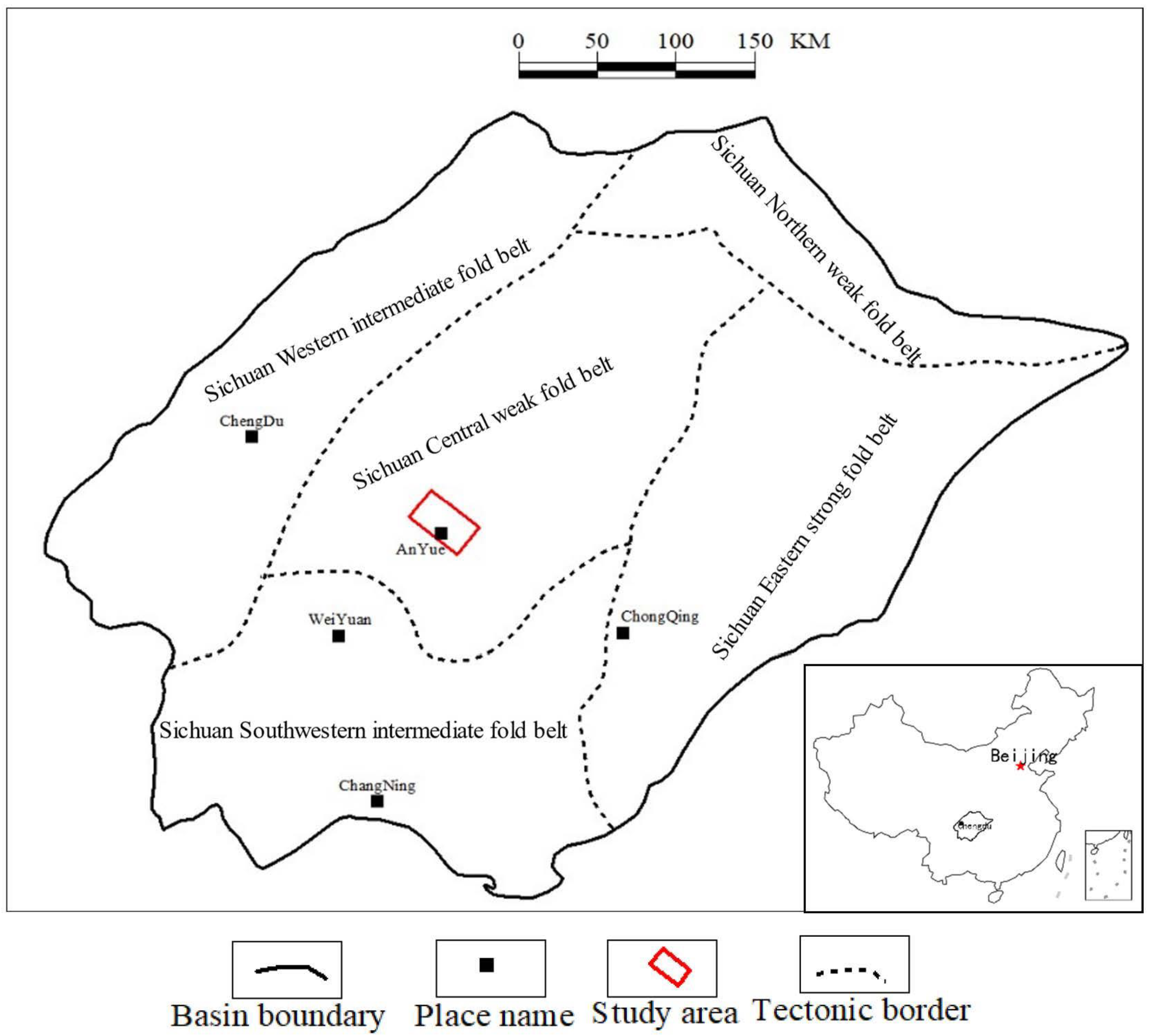
2. Geologic Settings

2.1. Structural Geology

The Sichuan Basin is a typical superimposed basin in southern China [59]. Since the late Indosinian period, the basin has experienced multi-stage strong tectonic movements in the Yanshanian and the Himalayan periods, resulting in the current tectonic pattern of the basin. According to the tectonic deformation intensity, the basin can be divided into five structural belts [60], including the middle strong fold belt in southwest Sichuan, the middle weak fold belt in middle Sichuan, the middle strong fold belt in west Sichuan, the weak fold belt in north Sichuan and the strong fold belt in east Sichuan. The study area is located in the weak fold belt in middle Sichuan (Figure 1), with no large faults, being at a higher position of structure in the paleo-structure, with a beneficial geologic condition for the formation of large gas fields. The gas reservoir of the Upper Triassic Xujiahe formation in the Anyue area of the Sichuan Basin is the largest tight sandstone gas reservoir discovered in the Sichuan Basin in recent years [61].

2.2. Sedimentary Geology

The tight sandstone reservoirs are Xu-2, Xu-4 and Xu-6, members of the Xujiahe formation (Figure 2). The sedimentary Triassic Xujiahe formation consists of shale and sandstone [62]. The sedimentary system is a braided river delta, and the effective reservoirs are mainly distributed in the microfacies of distributaries channels, mouth bars and shore-shallow lacustrine sand bars. The cumulative sandstone thickness is 200–340 m, with an average porosity of 7.24%. The types of reservoir space are inter-granular pore, inter-granular dissolved pore, matrix pore and micro-fracture [63]. The source rocks are dark mudstones of T₃X¹, T₃X³ and T₃X⁵ members, with a total thickness of more than 130 m [64].

3. Well Data

The study area covers 860 km², with 115 wells in which the drilling data and the conventional logging curves such as gamma-ray (GR), neutron porosity (NPHI), density (RHOB), P-sonic, caliper (CALI), compensated neutron log (CNL) and deep and shallow lateral resistivity are accessible. At the same time, S-sonic was available only in five wells (Figure 3), unsatisfied with the pre-stack dedicated reservoir description. Therefore, Well-1 to Well-4 were used as training wells, and Well-5 was used as a validation well to confirm the model’s reliability from deep learning.

4. Methodology and Workflow

As a type of machine learning, deep learning uses multi-layer nonlinear units to generate a multi-layer representation of data at different levels of abstraction. According to the system structure, it can learn representations and characteristics directly from the input without much prior knowledge, manual coding rules or engineering features [65]. The DFNN used the error backpropagation algorithm [66] to optimize the weight matrix of each layer (Figure 4). By comparing the error between the actual output and the expected output, the error signal was propagated from the output layer to the input layer to obtain the error signal of each layer, and then the weight coefficient of each layer was adjusted to reduce the error, thereby obtaining a new weight. Then, we adjusted the weight continuously to minimize the error to obtain the optimal weight coefficient.

The whole process includes the following steps (Figure 5):

1.

Data preparation and cleaning: The purpose of this step is to remove the abnormal values and eliminate the influence of the borehole environment on the input and target curve.

2.

Optimization of feature curves: XGBoost algorithm was used to automatically select the most important curve associated with the shear velocity as the final input curve for training.

3.

Construction of feedforward neural network: We constructed a deep feedforward neural network with multiple layers.

4.

Network fitting and evaluation: Because the weight and bias coefficients of the hidden layer cannot be obtained directly, the parameters of the network can be adjusted by comparing the errors between the results of the output layer and the expected output during the training process.

(a)

Based on the optimization of the activation and loss functions, the constructed network’s weight coefficient and bias were initialized randomly.

(b)

Forward propagation of the network: We imported the optimized feature curves into the input layer of the neural network, calculated the output value of the output layer (see Equations (1) and (2)), compared them with the expected output (shear velocity measured) and calculated the loss function value.

(c)

Network backpropagation: If the loss function value cannot meet the terminating condition, the output will be backpropagated layer-by-layer through the hidden layer to the input layer in a certain form, and the selected optimization algorithm will be used to allocate the error to all neurons in the front layers to obtain the error signal of each unit and as the basis for updating the weight coefficient and bias.

(d)

Suppose the loss function value meets the accuracy requirements or other terminating conditions, in that case, the training process and parameters updating should be ended, and the final network parameters can be saved for subsequent shear velocity prediction. Otherwise, steps (b) and (c) should be repeated.

$$z^{\left(l\right)}=W^{\left(l\right)}\cdot a^{\left(l-1\right)}+b^{\left(l\right)}$$

(1)

$$a^{\left(l\right)}=f_l\left(z^{\left(l\right)}\right)$$

(2)

The parameters are listed as follows:

• $f_l\left(·\right):$the activation function of neurons in l- layer
• $W^{\left(l\right)}\in {ℝ}^{m^{\left(l\right)}\times m^{l-1}}:$ the weight matrix of neurons from l-1 to l- layer
• $b^{\left(l\right)}$ the bias coefficient of neurons from the l-1 to l- layer
  $z^{\left(l\right)}\in {ℝ}^{m^l}:$ the net input of neurons in l- layer
• $a^{\left(l\right)}\in {ℝ}^{m^l}:$the output of neurons in l- layer

5. Data Cleaning and Preparation

The wells covering more intervals were selected to ensure that the data points used for training were representative and that the final model obtained by training was applicable. To ensure the correctness of the input feature curve, it was necessary to edit the logging data, mainly including the removal of abnormal values and standardization in multi-wells.

5.1. Removal of Outliers Values and Correction of Logging Curves

Invalid (null) logging data often appear at the top or bottom of the entire logging curve. Different logging series were measured in several runs, resulting in different depth ranges of null values for each curve. Therefore, before training, it was necessary to delete invalid values (Figure 6). The statistical results after deletion are shown in

Table 1. Statistical table after deleting abnormal values.

	CAL	CNL	RHOB	DTC	GR	lg_RT	lg_RXO	DTS
Count	11,391	11,391	11,391	11,391	11,391	11,391	11,391	11,391
Mean	6.73	0.12	2.57	63.75	94.27	1.60	1.60	106.20
Std	0.48	0.06	0.10	5.91	33.84	0.40	0.41	13.66
Min	4.02	0.01	1.68	49.99	33.97	0.49	0.38	83.54
Max	9.15	0.65	2.84	88.26	313.11	4.57	4.79	180.04

.

The reason for data correction is to reduce the instability of model training due to the error in data samples. Under the influence of a borehole environment, such as borehole collapse or mud invasion, logging data often fail to reflect the real information about the formation. Especially the RHOB curve, which was measured clinging to the borehole wall with a shallow detection depth, was easily affected by the borehole environment [67,68]. Therefore, these wrong data points need to be corrected. Figure 7 is the ccrossplot before and after correction. It shows that low-RHOB and high-NPHI data points were well corrected.

5.2. Optimization of Feature Curves

Feature selection is selecting effective features from the original feature curves to reduce the dimension of the data set, a key preprocessing step in machine learning and data mining [69,70]. In the case of high-dimensional data sets, using a feature curve owing to low correlation with the target curve will result in a low-quality model. There are several conventional logging curves; selecting the feature curve possessing a higher correlation with shear sonic curve before model training is necessary. With the XGBoost algorithm [71], the importance was ranked according to its gain value in all boosting decision trees. The importance of predicting the shear velocity increases with the growth of the F score. As shown in Figure 8, the order of importance is DTC < GR < CNL < RHOB < log (RT) < log (RS) < CAL. Therefore, the top five feature curves were selected according to the ranking of importance.

5.3. Multi-Well Standardization

The logging data in the study area were collected in different years. The logging histogram of the marker layer showed that the data distribution characteristics of different wells were inconsistent, especially in the DTC curve. Thus, before training the model, the histogram shifting method was used for multi-well standardization [72]. It can be seen from Figure 9 that after correction, the distribution shape of the same curve in different wells tends to be consistent.

5.4. Data Splitting

From the data set of Well-1 to Well-4, 70% of the data was randomly selected as the training set, and the remaining 30% was used as the test set (Figure 10) so that the training and testing could be carried out simultaneously in the subsequent model training.

5.5. Construction of the Network

A wide and deep neural network was constructed with five nodes in the input layer whose number is identical to selected feature curves and three hidden layers. The input layer is identical with the number of the selected feature curves; if we added more irrelevant curves, the accuracy and stability of the trained model would be downgraded. The number of neurons in each hidden layer is 32, the output layer has one node, and all layers are fully connected. The activation function of each layer is Elu, the loss function is MAE, and the parameter updating algorithm of the neural network is Adam. The trainable parameters of this network are up to 2337 (the optimization of the parameters for network construction will be discussed later). To compare the result, a shallow network was constructed in the same way, with only one hidden layer, 10 neurons in this layer and 71 trainable parameters. Comparing the training and test error curves of these two networks, the training and testing errors of the deep network are smaller than those of the shallow network, and the error curves are more stable (Figure 11).

6. Training

The difference (y-y’) between predicted output and expected output of GR, RHOB, P-sonic, neutron and log (RT) from four training wells was converted into loss function (J). When the training error of the neural network was large, the loss was high, while when it was small, the loss was low. The training goal is to find the weight matrix and bias vector to minimize the loss function on the training set.

6.1. Normalization of Input Curves

In almost machine learning algorithms, it is necessary to normalize the input characteristic curves. The neural network assumes that the input/output follows a normal distribution with an approximate mean value of zero and a variance of one. The purpose is to treat each feature fairly, make the subsequent optimization of solving weight parameters stable, eliminate dimensional influence, etc. The normalized data accelerate the convergence speed of the gradient descent algorithm [73]. The main normalization methods include z-score, min–max, decimal scaling, etc. The normalization methods were selected according to the statistical distribution shape of the feature curves, and the feature curves conformed to the normal distribution characteristics. Therefore, the z-score method was used (Equation (3)). After normalization, each input curve conformed to the normal distribution with the mean value of zero and the standard deviation of one (Figure 12). Figure 13 shows that the model trained by the normalized data has better generalization ability on the test data than the one from pre-normalized data.

$$z=\frac{x-\mathsf{\mu }}{\mathsf{\sigma }}$$

(3)

where $\mu \mathrm{is} \mathrm{the} \mathrm{average} \mathrm{value} \mathrm{of} \mathrm{the} \mathrm{feature} \mathrm{curve} \mathrm{and} \mathsf{\mu }=\frac{1}{N}{\displaystyle \sum }_{i=1}^N\left(x_i\right)$, N is the number of samples of a characteristic curve, and $x_i$ is the value at the i sample point of a feature curve; $\sigma \mathrm{is} \mathrm{the} \mathrm{standard} \mathrm{deviation} \mathsf{\sigma }=\sqrt{\frac{1}{N}{\displaystyle \sum }_{i=1}^N{\left(x_i-\mathsf{\mu }\right)}^2}$

6.2. Random Initialization of Model Parameters

Because the same activation function in the hidden layer is used in the network, if the parameters of each hidden unit are initialized to the same values, then for each hidden unit, the same value will be calculated according to the same input and passed to the output layer in the forward propagation. In backpropagation, the gradient value of each hidden unit is equal. Therefore, these parameters are still the same after multiple iterations using the gradient-based optimization algorithm. When the parameters are initialized to the same value, the parameters cannot be optimized through the gradient descent optimization algorithm. Therefore, the network’s model parameters (weight and bias parameters) are randomly initialized with small values. Then, the network parameters are updated according to the loss on the training data set through the optimization algorithm.

6.3. Selection of Loss Function

The loss function is used to estimate the error between the predicted value ($\widehat{y_i}$) and the real value $(y_i$). It is a non-negative real-value function usually expressed by L(Y, f(x)). The small value of the loss function indicates the more robustness of the model. The loss functions used for regression are mainly MAE and MSE. Because the relationship between MAE loss and the absolute error is linear, while the relation between MSE loss and error is square, when the error is large, MSE loss will be far greater than MAE loss. Therefore, when an abnormal value with a large error appears in the data, MSE will produce a very large loss, adversely influencing the model training. The logging data is still subject to acquisition noise even after the previous data cleaning and correction [74,75,76], so the MAE loss function was adopted, as shown in Equation (4).

$$J_{MAE}=\frac{1}{N}{\displaystyle \sum }_{i=1}^N\left|y_i-\widehat{y_i}\right|$$

(4)

6.4. Optimization of Activation Function

The activation function is used for adding a nonlinear effect, and only the nonlinear activation function can make the neural network approximate any complex function. The selection of activation function in the deep network influences training dynamics and task performance. The proper activation function can make gradient descent and backpropagation more effective, avoiding the exploding and vanishing gradient problems during the gradient calculation. Different activation functions have their specific application scenarios, drawbacks and strengths. Optimizing the activation function can help to achieve preferable results by neural network training.

The activation functions mainly include ReLU [77], Leaky-Relu [78], Selu [79], Gelu [80] and Elu [81]; their function, forms and effects are shown in

Table 2. Different activation function formulas and the effects.

Name of Activation Function	Formula	Effect
sigmoid	$\mathrm{sigmoid}\left(\mathrm{x}\right)=\mathsf{\sigma }=\frac{1}{1+{\mathrm{e}}^{-\mathrm{x}}}$	Its effect is to scale the output of each input neuron to 0–1.
ReLU	$\mathrm{ReLU}\left(\mathrm{x}\right)=\max \left(0,\mathrm{x}\right)$	If the input x is less than 0, then make the output equal to 0; otherwise, then make the output equal to the input.
Leaky-Relu	$\mathrm{LReLU}\left(\mathrm{x}\right)=\{\begin{array}{cc}\mathrm{x}& \mathrm{if} \mathrm{x}>0\\ \mathsf{\alpha }\mathrm{x}& \mathrm{if} \mathrm{x}\le 0\end{array}$	If input x is greater than 0, the output is x. If input x is less than or equal to 0, the output is α times the input.
Selu	$\mathrm{SELU}\left(\mathrm{x}\right)=\mathsf{\lambda }\{\begin{array}{cc}\mathrm{x}& \mathrm{if} \mathrm{x}>0\\ {\mathsf{\alpha }\mathrm{e}}^{\mathrm{x}}-\mathsf{\alpha }& \mathrm{if} \mathrm{x}\le 0\end{array}$	If the input value x is greater than 0, the output value is x times λ. If the input value x is less than 0, a singular function is obtained, which increases with the increase of x and approaches to the value when x is 0.
Gelu	$\mathrm{GELU}\left(\mathrm{x}\right)=0.5\mathrm{x}\left(1+\tanh \left(\sqrt{2/\mathsf{\pi }}\left(\mathrm{x}+0.044715{\mathrm{x}}^3\right)\right)\right)$	When x is greater than 0, the output is x, except for the interval from x = 0 to x = 1. At this time, the curve is more inclined to y-axis.
Elu	$\mathrm{ELU}\left(\mathrm{x}\right)=\{\begin{array}{cc}\mathrm{x}& \mathrm{if} \mathrm{x}>0\\ \mathsf{\alpha }\left({\mathrm{e}}^{\mathrm{x}}-1\right)& \mathrm{if} \mathrm{x}\le 0\end{array}$	The result is the same as that of ReLU; that is, the y value is equal to the x value, but if the input x is less than 0, we will obtain a value slightly less than 0. The parameter α can be adjusted as needed.

and Figure 14. In this paper, the activation function was optimized mainly based on the overall performance of the model in the training set and test set. Figure 15 shows that the ELU function performs best; the error curves in the training and test sets were smaller and more stable during each training epoch.

6.5. Optimization of Algorithm

After determining the feature curves, network and loss function, we needed an algorithm to search for the best possible parameter to minimize the loss function. The popularly used neural network optimization algorithm is the gradient descent algorithm. In each training step, a small amount of disturbance is made to each parameter, and the parameters are updated only when the loss of the training set is reduced. Most deep learning models do not have analytic solutions. Thus, we can only reduce the value of the loss function as much as possible by optimizing the model parameters with finite iterations. Nine optimization algorithms are widely used: Gradient Descent [82], Stochastic Gradient Descent [83], Mini Batch Gradient Descent [84], Momentum [85], Nestrov Accelerated Gradient [86], Adagrad [87], AdaDelta, RMSProp [43] and Adam [88]. The Adam method has its self-adapting learning rate and momentum for each parameter; thus during the training process, each parameter updating is independent, which improves the training speed and stability of the model. Adam is a modified Momentum + RMSProp algorithm, which can replace the first-order optimization algorithm of the traditional random gradient descent process. It can update the neural network weight iteratively based on the training data. By calculating the first-order and the second-order moment estimation of the gradient, independent adaptive learning rates are designed for different parameters and are robust for selected super parameters. Therefore, the Adam algorithm was used to update the network parameters iteratively.

7. Validation

The trained model (the final updated weight and bias) was applied to the prediction of shear velocity under the condition of input feature curves. This study uses a validation well with measured shear velocity to illustrate the model’s reliability. The prediction accuracy is compared with the shear velocity obtained by empirical formula and rock physics modeling, where the formula was obtained by fitting the measured S-sonic (the reciprocal of shear velocity) from P-sonic (the reciprocal of compressional velocity) (Figure 16); the correlation coefficient was 0.86, and the fitting formula is shown in Equation (5).

DTS = −6.64568 + 1.77482 × DTC

(5)

where DTC is the P-sonic curve with the unit of us/ft, and DTS is the S-sonic curve with the unit of us/ft.

Figure 17 shows that deep learning predicts the S-sonic curve and can better match the measured curve, especially in the layer with complex minerals (depth range from 2180–2235 m). With rock physics modeling, it is difficult to obtain an accurate mineral estimation result, and S-sonic’s prediction accuracy is relatively lower. According to the statistical histogram of S-sonic error (measured–predicted curve) (Figure 18), the error of empirical formula is between −10–10 us/ft, the error of petrophysical modeling is between −10–10 us/ft, and the error of deep learning is between −4–4 us/ft. As Vp/Vs is a prevailing indicator of lithology and fluid [89], it is crucial in evaluating unconventional reservoirs. Therefore, we focus on the accuracy comparison from Vp/Vs. The ccrossplot (Figure 19) shows that the V_p/V_s predicted by the deep learning method and the measured one can be better concentrated on the perfect fitting line of X = Y. At the same time, the Vp/Vs whose Vs was calculated by the empirical formula is a straight line, and that calculated by the Xu-White model also has a lower accuracy.

8. Conclusions and Further Work

In this study, based on quality control and correction of logging data, the feature curves were optimized automatically. By controlling the key steps in constructing the DFNN network, even without dropout and regularization, the network performed better in training and testing data. This shows that the model constructed by the DFNN method has good applicability and generalization ability. The comparative analysis of validation wells shows that the accuracy of deep learning is higher than that of empirical formula and rock physics modeling. The model for deep learning and training is derived from data; therefore, on the premise of a certain number of the reliable training set, this method not only can be used for shear velocity prediction of tight sandstone but also for shear velocity prediction under any other condition of complex lithology, and can be used for the formation evaluation with logging data as well.

References

1. Gholami, A.; Amirpour, M.; Ansari, H.R.; Seyedali, S.M.; Semnani, A.; Golsanami, N.; Heidaryan, E.; Ostadhassan, M. Porosity prediction from pre-stack seismic data via committee machine with optimized parameters. J. Pet. Sci. Eng. 2022, 210, 110067. [Google Scholar] [CrossRef]
2. Liu, L.; Geng, J.-H.; Guo, T.-L. The bound weighted average method (BWAM) for predicting S-wave velocity. Appl. Geophys. 2012, 9, 421–428. [Google Scholar] [CrossRef]
3. Qiu, T.; Xu, D.; Liu, J. Shear Wave Velocity Prediction of Glutenite Reservoir Based on Pore Structure Classification and Multiple Regression. In Proceedings of the 83rd EAGE Annual Conference & Exhibition, Madrid, Spain, 6–9 June 2022; pp. 1–5. [Google Scholar]
4. Zhang, Y.; Zhang, C.; Ma, Q.; Zhang, X.; Zhou, H. Automatic prediction of shear wave velocity using convolutional neural networks for different reservoirs in Ordos Basin. J. Pet. Sci. Eng. 2022, 208, 109252. [Google Scholar] [CrossRef]
5. Ghanbarnejad Moghanloo, H.; Riahi, M.A. Application of prestack Poisson dampening factor and Poisson impedance inversion in sand quality and lithofacies discrimination. Arab. J. Geosci. 2022, 15, 116. [Google Scholar] [CrossRef]
6. Ashraf, U.; Zhang, H.; Anees, A.; Ali, M.; Zhang, X.; Shakeel Abbasi, S.; Nasir Mangi, H. Controls on reservoir heterogeneity of a shallow-marine reservoir in Sawan Gas Field, SE Pakistan: Implications for reservoir quality prediction using acoustic impedance inversion. Water 2020, 12, 2972. [Google Scholar] [CrossRef]
7. Anees, A.; Zhang, H.; Ashraf, U.; Wang, R.; Liu, K.; Abbas, A.; Ullah, Z.; Zhang, X.; Duan, L.; Liu, F. Sedimentary facies controls for reservoir quality prediction of lower shihezi member-1 of the Hangjinqi area, Ordos Basin. Minerals 2022, 12, 126. [Google Scholar] [CrossRef]
8. Farfour, M.; Gaci, S.; El-Ghali, M.; Mostafa, M. A review about recent seismic techniques in shale-gas exploration. In Methods and Applications in Petroleum and Mineral Exploration and Engineering Geology; Elsevier: Amsterdam, The Netherlands, 2021; pp. 65–80. [Google Scholar]
9. Sohail, G.M.; Hawkes, C.D. An evaluation of empirical and rock physics models to estimate shear wave velocity in a potential shale gas reservoir using wireline logs. J. Pet. Sci. Eng. 2020, 185, 106666. [Google Scholar] [CrossRef]
10. Du, Q.; Yasin, Q.; Ismail, A.; Sohail, G.M. Combining classification and regression for improving shear wave velocity estimation from well logs data. J. Pet. Sci. Eng. 2019, 182, 106260. [Google Scholar] [CrossRef]
11. Castagna, J.P.; Batzle, M.L.; Eastwood, R.L. Relationships between compressional-wave and shear-wave velocities in clastic silicate rocks. Geophysics 1985, 50, 571–581. [Google Scholar] [CrossRef]
12. Domenico, S.N. Rock lithology and porosity determination from shear and compressional wave velocity. Geophysics 1984, 49, 1188–1195. [Google Scholar] [CrossRef]
13. Greenberg, M.; Castagna, J. Shear-wave velocity estimation in porous rocks: Theoretical formulation, preliminary verification and applications1. Geophys. Prospect. 1992, 40, 195–209. [Google Scholar] [CrossRef]
14. Han, D.-h.; Nur, A.; Morgan, D. Effects of porosity and clay content on wave velocities in sandstones. Geophysics 1986, 51, 2093–2107. [Google Scholar] [CrossRef]
15. Pickett, G.R. Acoustic character logs and their applications in formation evaluation. J. Pet. Technol. 1963, 15, 659–667. [Google Scholar] [CrossRef]
16. Tosaya, C.; Nur, A. Effects of diagenesis and clays on compressional velocities in rocks. Geophys. Res. Lett. 1982, 9, 5–8. [Google Scholar] [CrossRef]
17. Wang, P.; Peng, S. On a new method of estimating shear wave velocity from conventional well logs. J. Pet. Sci. Eng. 2019, 180, 105–123. [Google Scholar] [CrossRef]
18. Wyllie, M.; Gregory, A.; Gardner, G. An experimental investigation of factors affecting elastic wave velocities in porous media. Geophysics 1958, 23, 459–493. [Google Scholar] [CrossRef]
19. Ali, M.; Jiang, R.; Ma, H.; Pan, H.; Abbas, K.; Ashraf, U.; Ullah, J. Machine learning-A novel approach of well logs similarity based on synchronization measures to predict shear sonic logs. J. Pet. Sci. Eng. 2021, 203, 108602. [Google Scholar] [CrossRef]
20. Rajabi, M.; Hazbeh, O.; Davoodi, S.; Wood, D.A.; Tehrani, P.S.; Ghorbani, H.; Mehrad, M.; Mohamadian, N.; Rukavishnikov, V.S.; Radwan, A.E. Predicting shear wave velocity from conventional well logs with deep and hybrid machine learning algorithms. J. Pet. Explor. Prod. Technol. 2022, 1–24. [Google Scholar] [CrossRef]
21. Ali, M.; Ma, H.; Pan, H.; Ashraf, U.; Jiang, R. Building a rock physics model for the formation evaluation of the Lower Goru sand reservoir of the Southern Indus Basin in Pakistan. J. Pet. Sci. Eng. 2020, 194, 107461. [Google Scholar] [CrossRef]
22. Hou, B.; Chen, X.; Zhang, X. Critical porosity Pride model and its application. Shiyou Diqiu Wuli Kantan (Oil Geophys. Prospect.) 2012, 47, 277–281. [Google Scholar]
23. Lee, M.W. A simple method of predicting S-wave velocity. Geophysics 2006, 71, F161–F164. [Google Scholar] [CrossRef]
24. Xu, S.; Payne, M.A. Modeling elastic properties in carbonate rocks. Lead. Edge 2009, 28, 66–74. [Google Scholar] [CrossRef]
25. Xu, S.; White, R. A new velocity model for clay-sand mixtures: Geophysical Prospecting. Int. J. Rock Mech. Min. Sci. Geomech. Abstr. 1995, 7, 333A. [Google Scholar]
26. Mehrgini, B.; Izadi, H.; Memarian, H. Shear wave velocity prediction using Elman artificial neural network. Carbonates Evaporites 2019, 34, 1281–1291. [Google Scholar] [CrossRef]
27. Tabari, K.; Tabari, O.; Tabari, M. A fast method for estimating shear wave velocity by using neural network. Aust. J. Basic Appl. Sci. 2011, 5, 1429–1434. [Google Scholar]
28. Zahmatkesh, I.; Soleimani, B.; Kadkhodaie, A.; Golalzadeh, A.; Abdollahi, A.-M. Estimation of DSI log parameters from conventional well log data using a hybrid particle swarm optimization–adaptive neuro-fuzzy inference system. J. Pet. Sci. Eng. 2017, 157, 842–859. [Google Scholar] [CrossRef]
29. Akkurt, R.; Conroy, T.T.; Psaila, D.; Paxton, A.; Low, J.; Spaans, P. Accelerating and enhancing petrophysical analysis with machine learning: A case study of an automated system for well log outlier detection and reconstruction. In Proceedings of the SPWLA 59th Annual Logging Symposium, London, UK, 2–6 June 2018. [Google Scholar]
30. Silva, A.A.; Neto, I.A.L.; Misságia, R.M.; Ceia, M.A.; Carrasquilla, A.G.; Archilha, N.L. Artificial neural networks to support petrographic classification of carbonate-siliciclastic rocks using well logs and textural information. J. Appl. Geophys. 2015, 117, 118–125. [Google Scholar] [CrossRef]
31. Ashraf, U.; Zhang, H.; Anees, A.; Mangi, H.N.; Ali, M.; Zhang, X.; Imraz, M.; Abbasi, S.S.; Abbas, A.; Ullah, Z. A core logging, machine learning and geostatistical modeling interactive approach for subsurface imaging of lenticular geobodies in a clastic depositional system, SE Pakistan. Nat. Resour. Res. 2021, 30, 2807–2830. [Google Scholar] [CrossRef]
32. Hussain, M.; Liu, S.; Ashraf, U.; Ali, M.; Hussain, W.; Ali, N.; Anees, A. Application of Machine Learning for Lithofacies Prediction and Cluster Analysis Approach to Identify Rock Type. Energies 2022, 15, 4501. [Google Scholar] [CrossRef]
33. Sahoo, S.; Jha, M.K. Pattern recognition in lithology classification: Modeling using neural networks, self-organizing maps and genetic algorithms. Hydrogeol. J. 2017, 25, 311–330. [Google Scholar] [CrossRef]
34. Li, Y.; Anderson-Sprecher, R. Facies identification from well logs: A comparison of discriminant analysis and naïve Bayes classifier. J. Pet. Sci. Eng. 2006, 53, 149–157. [Google Scholar] [CrossRef]
35. Sebtosheikh, M.A.; Motafakkerfard, R.; Riahi, M.-A.; Moradi, S.; Sabety, N. Support vector machine method, a new technique for lithology prediction in an Iranian heterogeneous carbonate reservoir using petrophysical well logs. Carbonates Evaporites 2015, 30, 59–68. [Google Scholar] [CrossRef]
36. Shi, N.; Li, H.-Q.; Luo, W.-P. Data mining and well logging interpretation: Application to a conglomerate reservoir. Appl. Geophys. 2015, 12, 263–272. [Google Scholar] [CrossRef]
37. McCulloch, W.S.; Pitts, W. A logical calculus of the ideas immanent in nervous activity. Bull. Math. Biophys. 1943, 5, 115–133. [Google Scholar] [CrossRef]
38. Rosenblatt, F. The perceptron: A probabilistic model for information storage and organization in the brain. Psychol. Rev. 1958, 65, 386. [Google Scholar] [CrossRef]
39. Widrow, B.; Hoff, M.E. Adaptive switching circuits. in 1960 ire wescon convention record, 1960. reprinted in. Neurocomputing 1988, 49, 123. [Google Scholar]
40. Rumelhart, D.E. Learning internal representations by error propagation. In Parallel Distributed Processing: Explorations in the Microstructure of Cognition; MIT Press: Cambridge, MA, USA, 1986; pp. 318–362. [Google Scholar]
41. LeCun, Y.; Touresky, D.; Hinton, G.; Sejnowski, T. A theoretical framework for back-propagation. In Proceedings of the 1988 Connectionist Models Summer School; Morgan Kaufmann: San Mateo, CA, USA, 1988; pp. 21–28. [Google Scholar]
42. Hochreiter, S.; Schmidhuber, J. Long short-term memory. Neural Comput. 1997, 9, 1735–1780. [Google Scholar] [CrossRef]
43. Hinton, G. Graduate Summer School: Deep learning, Feature Learning. 2012. Available online: https://www.ipam.ucla.edu/schedule.aspx?pc=gss2012 (accessed on 24 August 2022).
44. Bengio, Y.; LeCun, Y. Scaling learning algorithms towards AI. Large-Scale Kernel Mach. 2007, 34, 1–41. [Google Scholar]
45. Ranzato, M.A.; Boureau, Y.-L.; Cun, Y. Sparse feature learning for deep belief networks. In Proceedings of the Twenty-First Annual Conference on Neural Information Processing Systems, Vancouver, BC, Canada, 3–6 December 2007. [Google Scholar]
46. Delalleau, O.; Bengio, Y. Shallow vs. deep sum-product networks. In Proceedings of the 25th Annual Conference on Neural Information Processing Systems 2011, Granada, Spain, 12–14 December 2011. [Google Scholar]
47. Montufar, G.F.; Pascanu, R.; Cho, K.; Bengio, Y. On the number of linear regions of deep neural networks. In Proceedings of the Annual Conference on Neural Information Processing Systems 2014, Montreal, QC, Canada, 8–13 December 2014. [Google Scholar]
48. Pascanu, R.; Gulcehre, C.; Cho, K.; Bengio, Y. How to construct deep recurrent neural networks. arXiv 2013, arXiv:1312.6026. [Google Scholar]
49. Ashraf, U.; Zhang, H.; Anees, A.; Nasir Mangi, H.; Ali, M.; Ullah, Z.; Zhang, X. Application of unconventional seismic attributes and unsupervised machine learning for the identification of fault and fracture network. Appl. Sci. 2020, 10, 3864. [Google Scholar] [CrossRef]
50. Meshalkin, Y.; Koroteev, D.; Popov, E.; Chekhonin, E.; Popov, Y. Robotized petrophysics: Machine learning and thermal profiling for automated mapping of lithotypes in unconventionals. J. Pet. Sci. Eng. 2018, 167, 944–948. [Google Scholar] [CrossRef]
51. Li, S.; Liu, B.; Ren, Y.; Chen, Y.; Yang, S.; Wang, Y.; Jiang, P. Deep-learning inversion of seismic data. arXiv 2019, arXiv:1901.07733. [Google Scholar] [CrossRef]
52. Liu, M.; Grana, D. Accelerating geostatistical seismic inversion using TensorFlow: A heterogeneous distributed deep learning framework. Comput. Geosci. 2019, 124, 37–45. [Google Scholar] [CrossRef]
53. Richardson, A. Seismic full-waveform inversion using deep learning tools and techniques. arXiv 2018, arXiv:1801.07232. [Google Scholar]
54. Sacramento, I.; Trindade, E.; Roisenberg, M.; Bordignon, F.; Rodrigues, B.B. Acoustic impedance deblurring with a deep convolution neural network. IEEE Geosci. Remote Sens. Lett. 2018, 16, 315–319. [Google Scholar] [CrossRef]
55. Feng, R. Estimation of reservoir porosity based on seismic inversion results using deep learning methods. J. Nat. Gas Sci. Eng. 2020, 77, 103270. [Google Scholar] [CrossRef]
56. Chen, Y.; Zhang, G.; Bai, M.; Zu, S.; Guan, Z.; Zhang, M. Automatic waveform classification and arrival picking based on convolutional neural network. Earth Space Sci. 2019, 6, 1244–1261. [Google Scholar] [CrossRef] [Green Version]
57. Yuan, S.; Liu, J.; Wang, S.; Wang, T.; Shi, P. Seismic waveform classification and first-break picking using convolution neural networks. IEEE Geosci. Remote Sens. Lett. 2018, 15, 272–276. [Google Scholar] [CrossRef]
58. Smith, R.; Mukerji, T.; Lupo, T. Correlating geologic and seismic data with unconventional resource production curves using machine learning. Geophysics 2019, 84, O39–O47. [Google Scholar] [CrossRef]
59. Jiang, R.; Zhao, L.; Xu, A.; Ashraf, U.; Yin, J.; Song, H.; Su, N.; Du, B.; Anees, A. Sweet spots prediction through fracture genesis using multi-scale geological and geophysical data in the karst reservoirs of Cambrian Longwangmiao Carbonate Formation, Moxi-Gaoshiti area in Sichuan Basin, South China. J. Pet. Explor. Prod. Technol. 2022, 12, 1313–1328. [Google Scholar] [CrossRef]
60. Kangling, D. Formation and evolution of Sichuan Basin and domains for oil and gas exploration. Nat. Gas Ind. 1992, 12, 7–12. [Google Scholar]
61. Huang, X.; Zhang, L.; Zheng, W.; Xiang, X.; Wang, G. Controlling Factors of Gas Well Deliverability in the Tight Sand Gas Reservoirs of the Upper Submember of the Second Memher of the Upper Triassic Xujiahe Formation in the Anyue Area, Sichuan Basin. Nat. Gas Ind. 2012, 32, 65. [Google Scholar]
62. Ullah, J.; Luo, M.; Ashraf, U.; Pan, H.; Anees, A.; Li, D.; Ali, M.; Ali, J. Evaluation of the geothermal parameters to decipher the thermal structure of the upper crust of the Longmenshan fault zone derived from borehole data. Geothermics 2022, 98, 102268. [Google Scholar] [CrossRef]
63. Li, M.; Lai, Q.; Huang, K. Logging identification of fluid properties in low porosity and low permeability clastic reservoir: A case study of Xujiahe Fm gas reservoirs in the Anyue gas field, Sichuan basin. Nat. Gas Ind. 2013, 33, 34–38. (In Chinese) [Google Scholar]
64. Zeng, Q.; Gong, C.; Li, J.; Che, G.; Lin, J. Exploration achievements and potential analysis of gas reservoirs in the Xujiahe formation, central Sichuan Basin. Nat. Gas Ind. 2009, 29, 13–18. [Google Scholar]
65. Xu, C.; Misra, S.; Srinivasan, P.; Ma, S. When petrophysics meets big data: What can machine do? In Proceedings of the SPE Middle East Oil and Gas Show and Conference, Manama, Bahrain, 18–21 March 2019. [Google Scholar]
66. Rumbert, D. Learning internal representations by error propagation. Parallel Distrib. Process. 1986, 1, 318–363. [Google Scholar]
67. de Macedo, I.A.; de Figueiredo, J.J.S.; De Sousa, M.C. Density log correction for borehole effects and its impact on well-to-seismic tie: Application on a North Sea data set. Interpretation 2020, 8, T43–T53. [Google Scholar] [CrossRef]
68. Ugborugbo, O.; Rao, T. Impact of borehole washout on acoustic logs and well-to-seismic ties. In Proceedings of the Nigeria Annual International Conference and Exhibition, Abuja, Nigeria, 3 August 2009. [Google Scholar]
69. Anifowose, F.A.; Labadin, J.; Abdulraheem, A. Non-linear feature selection-based hybrid computational intelligence models for improved natural gas reservoir characterization. J. Nat. Gas Sci. Eng. 2014, 21, 397–410. [Google Scholar] [CrossRef]
70. Tao, Z.; Huiling, L.; Wenwen, W.; Xia, Y. GA-SVM based feature selection and parameter optimization in hospitalization expense modeling. Appl. Soft Comput. 2019, 75, 323–332. [Google Scholar] [CrossRef]
71. Chen, T.; Guestrin, C. Xgboost: A scalable tree boosting system. In Proceedings of the Proceedings of the 22nd Acm Sigkdd International Conference on Knowledge Discovery and Data Mining, San Francisco, CA, USA, 13–17 August 2016; pp. 785–794. [Google Scholar]
72. Lideng, G.; Xiaofeng, D.; Zhang, X.; Linggao, L.; Wenhui, D.; Xiaohong, L.; Yinbo, G.; Minghui, L.; Shufang, M.; HUANG, Z. Key technologies for seismic reservoir characterization of high water-cut oilfields. Pet. Explor. Dev. 2012, 39, 391–404. [Google Scholar]
73. Ioffe, S.; Szegedy, C. Batch normalization: Accelerating deep network training by reducing internal covariate shift. In Proceedings of the International Conference on Machine Learning, Lille, France, 6–11 July 2015; pp. 448–456. [Google Scholar]
74. Al-Farisi, O.; Dajani, N.; Boyd, D.; Al-Felasi, A. Data management and quality control in the petrophysical environment. In Proceedings of the Abu Dhabi International Petroleum Exhibition and Conference, Abu Dhabi, United Arab Emirates, 11–14 October 2002. [Google Scholar]
75. Kumar, M.; Dasgupta, R.; Singha, D.K.; Singh, N. Petrophysical evaluation of well log data and rock physics modeling for characterization of Eocene reservoir in Chandmari oil field of Assam-Arakan basin, India. J. Pet. Explor. Prod. Technol. 2018, 8, 323–340. [Google Scholar] [CrossRef]
76. Theys, P.; Roque, T.; Constable, M.V.; Williams, J.; Storey, M. Current status of well logging data deliverables and a vision forward. In Proceedings of the SPWLA 55th Annual Logging Symposium, Abu Dhabi, United Arab Emirates, 18–22 May 2014. [Google Scholar]
77. Jarrett, K.; Kavukcuoglu, K.; Ranzato, M.A.; LeCun, Y. What is the best multi-stage architecture for object recognition? In Proceedings of the 2009 IEEE 12th International Conference on Computer Vision, Kyoto, Japan, 29 September–2 October 2009; pp. 2146–2153. [Google Scholar]
78. Maas, A.L.; Hannun, A.Y.; Ng, A.Y. Rectifier nonlinearities improve neural network acoustic models. In Proceedings of the ICML, Atlanta, GA, USA, 16–21 June 2013; p. 3. [Google Scholar]
79. Klambauer, G.; Unterthiner, T.; Mayr, A.; Hochreiter, S. Self-normalizing neural networks. In Proceedings of the Annual Conference on Neural Information Processing Systems 2017, Long Beach, CA, USA, 4–9 December 2017. [Google Scholar]
80. Hendrycks, D.; Gimpel, K. Gaussian error linear units (gelus). arXiv 2016, arXiv:1606.08415. [Google Scholar]
81. Clevert, D.-A.; Unterthiner, T.; Hochreiter, S. Fast and accurate deep network learning by exponential linear units (elus). arXiv 2015, arXiv:1511.07289. [Google Scholar]
82. Hochreiter, S.; Younger, A.S.; Conwell, P.R. Learning to learn using gradient descent. In Proceedings of the International Conference on Artificial Neural Networks, Vienna, Austria, 21–25 August 2001; pp. 87–94. [Google Scholar]
83. Darken, C.; Chang, J.; Moody, J. Learning rate schedules for faster stochastic gradient search. In Proceedings of the Neural Networks for Signal Processing, Helsingoer, Denmark, 31 August–2 September 1992. [Google Scholar]
84. Khirirat, S.; Feyzmahdavian, H.R.; Johansson, M. Mini-batch gradient descent: Faster convergence under data sparsity. In Proceedings of the 2017 IEEE 56th Annual Conference on Decision and Control (CDC), Melbourne, Australia, 12–15 December 2017; pp. 2880–2887. [Google Scholar]
85. Rumelhart, D.E.; Hinton, G.E.; Williams, R.J. Learning representations by back-propagating errors. Nature 1986, 323, 533–536. [Google Scholar] [CrossRef]
86. Nesterov, Y. Gradient methods for minimizing composite functions. Math. Program. 2013, 140, 125–161. [Google Scholar] [CrossRef]
87. Duchi, J.; Hazan, E.; Singer, Y. Adaptive subgradient methods for online learning and stochastic optimization. J. Mach. Learn. Res. 2011, 12, 2121–2159. [Google Scholar]
88. Kingma, D.P.; Ba, J. Adam: A method for stochastic optimization. arXiv 2014, arXiv:1412.6980. [Google Scholar]
89. Liu, K.; Sun, J.; Zhang, H.; Liu, H.; Chen, X. A new method for calculation of water saturation in shale gas reservoirs using VP-to-VS ratio and porosity. J. Geophys. Eng. 2018, 15, 224–233. [Google Scholar] [CrossRef] [Green Version]
Figure 1. Regional tectonic background and location of the study area in the Sichuan central weak fold belt. The study area of Anyue Gas Field is a reputable gas field in China.
Energies 15 07016 g001
Figure 2. Stratigraphy of Triassic and Jurassic in the study area. The Triassic Xujiahe formation is the target formation.
Energies 15 07016 g002
Figure 3. Base map of the study area (the red square is the boudary of the project shown in the Figure 1). The wells utilized in the study are written by their names.
Energies 15 07016 g003
Figure 4. Schematic diagram of network propagation (Wi is the weight coefficient matrix, fi is the nonlinear activation function).
Energies 15 07016 g004
Figure 5. The workflow shows the necessary steps adopted to complete the study.
Energies 15 07016 g005
Figure 6. Detection of abnormal values (yellow for null, blue for non-null).
Energies 15 07016 g006
Figure 7. Crossplot of CNL and RHOB logging before (a) and after (b) the correction (color-coded by caliper curve).
Energies 15 07016 g007
Figure 8. Bar graph for ranking the importance of the feature curve.
Energies 15 07016 g008
Figure 9. Comparison of statistical histogram pre- and post-multi-well standardization of input feature curves. The upper figure is a histogram of preprocessing, and the lower figure is a histogram of post-processing.
Energies 15 07016 g009
Figure 10. Splitting of a data set showing the 70% training data and the 30% testing data set.
Energies 15 07016 g010
Figure 11. Comparison of prediction errors between the deep network and the shallow network: (a) shallow network diagram; (b) deep network diagram; (c) trainable parameters of the shallow network; (d) trainable parameters of deep network; (e) training error (blue curve) and test error (red curve) of the shallow network; (f) training error (blue curve) and test error (red curve) of deep network.
Energies 15 07016 g011
Figure 12. Comparison of statistical characteristics of feature curves before and after normalization. The sub-figures on the left side shows the logs before normalization (a) Density, (c) CNL, (e) log(RT), (g) DTC, (i) GR. Whereas, the subfigures on the right side shows logs after normalization (b) Density, (d) CNL, (f) log(RT), (h) DTC, (j) GR.
Energies 15 07016 g012
Figure 13. Comparison of learning curves before (a) and after (b) normalization: blue curves represent the error on the trained data, red curves represent the error on the test data.
Energies 15 07016 g013
Figure 14. Images of different activation functions (a) and their derivatives (b).
Energies 15 07016 g014
Figure 15. Errors of different activation functions in the training set (a) and test set (b).
Energies 15 07016 g015
Figure 16. Crossplot of S-sonic and P-sonic and their linear fitting.
Energies 15 07016 g016
Figure 17. Comparison of S-sonic curves predicted by different methods (dts_emp, DTS_RM, KERAS_DTS were calculated, respectively, by the empirical formula, the rock physics modeling method, deep learning, and DTS is the measured S-sonic curve).
Energies 15 07016 g017
Figure 18. Statistical histogram of S-sonic errors predicted by different methods: (a) Empirical formula, (b) Rock physics modeling, (c) Deep learning.
Energies 15 07016 g018
Figure 19. Crossplot of Vp/Vs predicted by different methods ((a) Empirical formula, (b) Rock physics modeling, (c) Deep learning) and measured Vp/Vs in well validation.
Energies 15 07016 g019