Method to Estimate Thermal Transients in Reactors and Determine Their Parameter Sensitivities without a Forward Simulation

Abstract

Thermal response time is an important parameter for the control of fast reactors. Modern thermal hydraulic codes allow for the modeling of transient responses and can also be used to understand the dominant factors that affect them. However, simulations can be computationally expensive, particularly for performing parametric analyses of how thermophysical properties affect transient behavior. Here, we present a method for using linear stability analysis to estimate thermal response time and determine the key parameters that affect transient behavior without performing a forward simulation. The approach can also be used to corroborate simulation results and is tested against simulation results produced with a 2D finite difference model. The results show that this approach produces time-dependent temperature profiles that are within 2 × 10⁻⁵–0.1% of the numerical results for a single node perturbation. Changes in temperature have the greatest effect on thermal response time, followed by changes to thermal conductivity.

1. Introduction

Accurately modeling heat transfer in a nuclear reactor core is central to understanding safety and performance. While thermal transport directly affects in-core material temperatures, it also affects the stability of the reactor due to the strong feedback between neutron multiplication, fuel, and coolant temperatures. Increases in fuel temperature tend to lower core reactivity due to the Doppler broadening of neutron absorption resonances in ²³⁸U. In contrast, changes in coolant temperature have effects on reactivity that strongly depend on coolant type and core geometry [1]. Fuel compositions evolve over time in a reactor due to the high temperatures and radiation fields. Properties such a porosity are difficult to measure but can have huge impacts on the thermal conductivity of fuel, resulting in changes in thermal response over the lifetime of the fuel.

Multiple codes exist for transient thermal analysis (e.g., ASTEC-Na/CESAR, RELAP5, SIMMER, CATHARE, SAS-SFR, and many others) [2,3,4,5,6,7,8,9,10,11]. However, they can be computationally expensive to run, especially for understanding which thermophysical parameters are dominant. Many of the codes in this domain are also coupled to larger packages that allow for neutronic or systems analysis. Validating the results of these codes is always important, as is understanding the dominant parameters that affect transient behavior.

A method with which to estimate thermal transient behavior, and the dominant factors affecting it, that does not require a complete thermal hydraulic simulation would be of significant value. Here, we present a method for using linear perturbation analysis to do exactly this. Linear perturbation methods have been used in reactor physics to understand the stability of LWRs [12,13,14] and fast reactors [15,16] to thermal perturbations or the insertion of reactivity. The approach has been to formulate a set of equations for reactivity and its coupling to temperature in the core, which itself can be modeled simply as a thermal resistor network [13]. A linearized set of differential equations can then be formed whose eigenvalues provide the stability of the system to perturbations. A similar approach has found broad use for understanding the flow instabilities in BWRs. The onset of density wave oscillations has been modeled in this way [17,18,19], as it has with super critical water reactors [20,21,22,23]. Linear stability analysis has also been used to understand natural circulation in purely thermal hydraulic systems related to reactors [24]. The technique in these types of applications has its origins in understanding fluid instabilities, in general [25,26]. Recent advances in the application of linear stability analysis to fission waves have also shown that it can be used to understand the parameter space where stability, instability, and Hopf bifurcations can arise [27].

The use of linear perturbation theory here is not for understanding the rise of instabilities that leads to changes in flow regime; rather, the eigenvalues of the Jacobian are used in conjunction with the perturbation to create an eigenfunction expansion that can be used to predict the temporal behavior of the temperature and its related properties. When used in this way, the eigenvalues of the Jacobian can be used to directly estimate thermal trajectories. This is useful in systems where computation is expensive, but also to verify computational results even where it is not. However, the real virtue of this approach is that it can be directly used to determine the dominant factors affecting thermal transients and the parameter sensitivities of these transient phenomena. The Jacobian can also be used to produce a covariance matrix that shows how the trajectory of variables relate to one another [28].

2. Materials and Methods

Here, we consider thermal transients in a sodium-cooled fast reactor and use open-source information on the BN800 fuel as a reference. A finite difference model for thermal transport in a fuel pin is used to estimate the terms in a Jacobian matrix when a thermal transient occurs without the need to complete a forward calculation beyond one time step. The eigenvalues from the Jacobian can then be used to estimate the trajectory of the temperature and thermophysical properties. The results are validated against a full forward simulation of the finite difference model that was, itself, validated using the results of the CABRI BI1 experiment [29] whose design parameters are given in Supplementary Note S1 and Table S1.

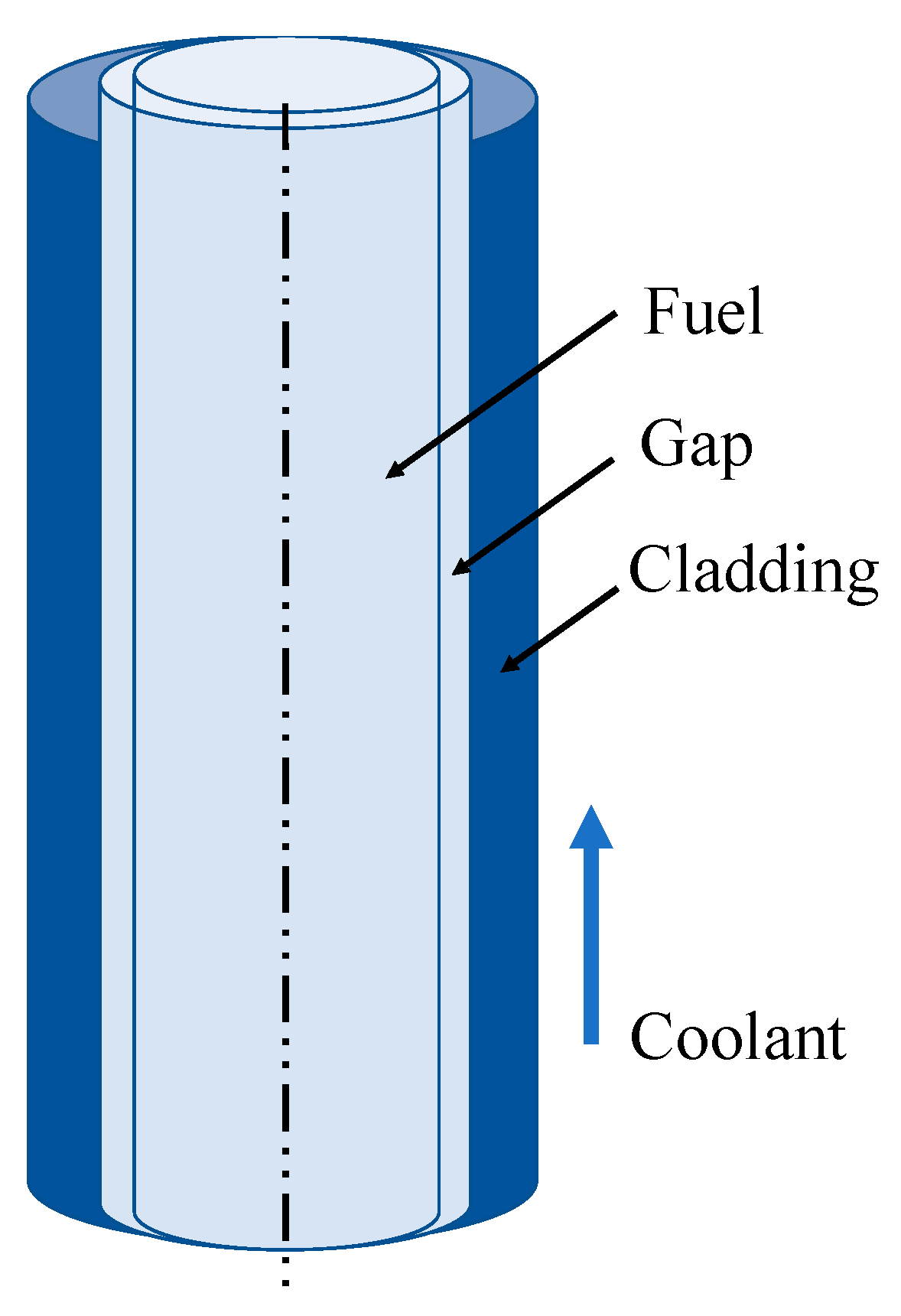
2.1. Fuel Parameters and Numerical Simulations

Table 1. Design parameters for the mixed oxide reactor based on a BN-800 reactor [33]. * corresponds to calculated values.

Core	Mixed Oxide
Fuel form	UPuO2
Coolant	Sodium
Cladding	Steel
Gap fill	Helium
Inlet coolant temperature (K)	627.15
Average linear power (kW/m)	31
Initial coolant mass flow rate * (kg/s)	0.1786
Fissile section height (cm)	88
Cladding thickness (cm)	0.04
Gap thickness * (cm)	0.001158
Pin diameter (cm)	0.66
Hexagonal lattice pitch * (cm)	0.8662

provides the properties for the BN800 MOX fuel and coolant. The thermophysical properties used come from open literature, with the fuel thermal conductivity and density properties coming from [30], the fuel specific heating coming from [30,31] for the U and Pu dioxide correlations, the gap thermal conductivity from [32], the cladding properties from [33], the coolant density and specific heat from [31], and the coolant dynamic viscosity from [34]. The convective heat transfer correlations between the outer cladding surface and the coolant are obtained from a Nusselt number correlation based on the pitch to diameter ratio of 1.31 [33]. The Ross and Stout gap heat transfer coefficient model is also used [33]. The material thermophysical properties vary both axially and radially.

For the linear stability analysis and finite difference model, we consider a single fuel pin (Figure 1) with 18 axial nodes and 121 radial nodes. Of the latter, 100 radial nodes are in the fuel, 20 in the cladding, and 1 is in the coolant, as in the previous finite difference forward stepping model. For the numerical simulation, a time step of 0.0001 s is used. Supplementary Note S1 provides the details on the convergence test used to determine the time step size and node spacing.

A Crank–Nicolson discretization scheme is used for the numerical simulation. The initial governing equations and the discretized forms are provided in Supplementary Note S1. The numerical simulation was benchmarked against the CABRI BI1 experiment and SAS-SFR model of the experiment [29]. Details of the CABRI validation, as well as the additional crosschecks, are provided in Supplementary Note S1.

2.2. Linear Stability Model

The Jacobian-based sensitivity analysis comes from a linear stability model and is consistent with the formulation developed by Cady and Kenton (1983) [35]. This model uses the same node spacing and design parameters as the numerical simulation. One starts with a vector, $\stackrel{\rightharpoonup }{F}$, of the temporal derivatives of temperatures and properties within the system, Equation (1). Here, we look at the setup for a single node. For the full system, terms are added for all nodes being considered. The trajectory of the system properties can be written as:

$$\stackrel{\rightharpoonup }{F}=\frac{\partial \stackrel{\rightharpoonup }{f}}{\partial t}=\left[\begin{array}{c}\frac{\partial T}{\partial t}\\ \frac{\partial k}{\partial t}\\ \frac{\partial \rho }{\partial t}\\ \frac{\partial c_p}{\partial t}\end{array}\right]$$

(1)

Stability analyses are done around the fixed points determined from the steady-state system:

$$\stackrel{\rightharpoonup }{f^{*}}=\left[\begin{array}{c}{T}^{*}\\ k^{*}\\ {\rho }^{*}\\ c_p{}^{*}\end{array}\right]$$

(2)

The perturbation, $\stackrel{\rightharpoonup }{f^{\prime }}$, is the difference in the current vector, $\stackrel{\rightharpoonup }{f}$, and the fixed-point vector:

$$\stackrel{\rightharpoonup }{f^{\prime }}=\stackrel{\rightharpoonup }{f}-\stackrel{\rightharpoonup }{f^{*}}$$

(3)

Using a first-order linear stability approximation evolution of the perturbation, it can be written as [36]:

$$\frac{\partial \stackrel{\rightharpoonup }{f^{\prime }}}{\partial t}=\left(J\stackrel{\rightharpoonup }{F}\right)\stackrel{\rightharpoonup }{f^{*}}$$

(4)

where the Jacobian, denoted by J, whose eigenvalues can be used to estimate the temporal response of temperature, specific heat, density, and thermal conductivity is given by:

$$J\stackrel{\rightharpoonup }{F}=\left[\begin{array}{c}\left(\frac{\partial }{\partial T}\frac{\partial T}{\partial t}\right)\left(\frac{\partial }{\partial \rho }\frac{\partial T}{\partial t}\right)\left(\frac{\partial }{\partial c_p}\frac{\partial T}{\partial t}\right)\left(\frac{\partial }{\partial k}\frac{\partial T}{\partial t}\right)\\ \left(\frac{\partial }{\partial T}\frac{\partial k}{\partial t}\right)\left(\frac{\partial }{\partial k}\frac{\partial k}{\partial t}\right)\left(\frac{\partial }{\partial \rho }\frac{\partial k}{\partial t}\right)\left(\frac{\partial }{\partial c_p}\frac{\partial k}{\partial t}\right)\\ \left(\frac{\partial }{\partial T}\frac{\partial \rho }{\partial t}\right)\left(\frac{\partial }{\partial k}\frac{\partial \rho }{\partial t}\right)\left(\frac{\partial }{\partial \rho }\frac{\partial \rho }{\partial t}\right)\left(\frac{\partial }{\partial c_p}\frac{\partial \rho }{\partial t}\right)\\ \left(\frac{\partial }{\partial T}\frac{\partial c_p}{\partial t}\right)\left(\frac{\partial }{\partial k}\frac{\partial c_p}{\partial t}\right)\left(\frac{\partial }{\partial \rho }\frac{\partial c_p}{\partial t}\right)\left(\frac{\partial }{\partial c_p}\frac{\partial c_p}{\partial t}\right)\end{array}\right]$$

(5)

The derivatives are applied directly to the thermophysical properties with explicit equations. Where analytical expressions for terms are not available, the partial derivatives are estimated using the finite difference equations for temperature. Here, the explicit Euler method is utilized instead of the Crank–Nicolson method used with the finite difference simulations [29]. Details of the derivation of each term in Equation (5) are provided in Supplementary Note S2. This matrix expands to include all four variables of Equation (2) for every location within the fuel pin, except for the nodes in the coolant. The coolant nodes could be included in a future iteration of this model in order to provide axial coupling. However, the coolant temperatures are not included in the Jacobian because they are not significantly impacted by the perturbations used in this analysis.

A first-order linear stability analysis provides a solution for the time evolution of perturbations to system parameters [36]:

$${\epsilon }_j\left(t\right)={\displaystyle \sum }_{n=1}^N{c}_n{e}^{{\lambda }_{n}t}{\eta }_{j,n}$$

(6)

Here, ${\epsilon }_j$ represents the perturbations to the parameters in $\stackrel{\rightharpoonup }{f^{\prime }}$, c_n represents the constants, λ_n represents the eigenvalues of the Jacobian, and η_j,n represents the corresponding eigenvectors specific to the nodal location j. The constants, c_n, are determined using:

$${\epsilon }_j\left(t_0+∆t\right)-{\epsilon }_j\left(t_0\right)=∆{\epsilon }_j={\displaystyle \sum }_{n=1}^N{c}_n{e}^{{\lambda }_n\left(t_0+∆t\right)}{\eta }_{j,n}-{\displaystyle \sum }_{n=1}^N{c}_n{e}^{{\lambda }_n{t}_0}{\eta }_{j,n}$$

(7)

Equation (7) can then be written as:

$$∆{\epsilon }_j={\displaystyle \sum }_{n=1}^N c_n e^{{\lambda }_n{t}_0} (e^{{\lambda }_n∆t}-1){\eta }_{j,n}$$

(8)

Here, the ∆ε_j terms are the perturbed values of the respective parameters in Equation (2), and the time step, ∆t, corresponds to the time step used in the finite difference model. Starting from a stable system where ${\epsilon }_j\left(t_0\right)=0$ and $t_0=0$, and assuming the perturbation is applied instantaneously as in the simulations presented here, Equation (8) can be simplified as follows:

$${\epsilon }_j\left(∆t\right)={\displaystyle \sum }_{n=1}^N{c}_n{\eta }_{j,n} (e^{{\lambda }_n∆t}-1)$$

(9)

If the perturbation is close enough to the fixed point, then the eigenvalues of the Jacobian, Equation (5), can be used in Equation (9), or more generally Equation (8), which can be represented as a matrix equation and solved for the constants c_n. Here, the standard Matlab function eig is used [37]. The coolant nodes are not considered in the Jacobian, and we use 120 radial (100 in the fuel and 20 in the cladding) and 18 axial nodes, for a total of 2160 nodes. The time step used for the results with a single node being perturbed is 0.0001 s. When the entire centerline of the fuel is perturbed, a longer simulation time is needed; therefore, the time step is increased to 0.001 s. The axial mesh size is 4.89 cm. In the radial direction, the distance between the nodes in the fuel is 0.00292 cm, and in the cladding, it is 0.00211 cm.

3. Results and Discussion

Figure 2, Figure 3, Figure 4 and Figure 5 show a comparison of the simulation results with the approximations from the linear stability analysis (Equation (6)). In Figure 2, the temporal response of the peak temperature in the fuel pin is shown for four different perturbations at that location: + 0.01% T_initial, + 0.1% T_initial, + 1.0% T_initial, and + 3% T_initial. This represents a perturbation applied to the volume of fuel associated with the peak temperature. For all perturbation cases, the difference between the new eigen solution result and the finite difference model results were 1.91 × 10⁻⁵%, or less, at 0.01 s.

Similar results can be seen for the three main properties of the system: thermal conductivity, density, and specific heat (Figure 3). The results align well, but we can start to see the differences between the linear stability approach and the finite difference simulations as the perturbations increase towards 3%. This is expected as stability models based on eigen solutions are only guaranteed to hold true for small perturbations. For all thermophysical properties with perturbations of 1% or lower, the difference between the new steady-state value the eigen solution reaches and the finite difference model results were 1.30 × 10⁻²%, or less, at 0.01 s.

For the 3% perturbation, the maximum difference was 0.116% (only for thermal conductivity). The difference between the performance of the linear stability approach for thermal conductivity, relative to specific heat and density, stems from the concave nature of the k(T) over the temperature range in the simulations. This functional shape is inherently less amenable to linear stability modeling.

To confirm that the eigen solution successfully models the thermal response behavior across an entire axial section of the fuel, Figure 4 shows the finite difference model and Jacobian temperature results for nodes radially across from the 1% centerline perturbation at the outer fuel, inner cladding, and outer cladding nodes. The percent differences between the models at 1 s are all in the order of 10⁻⁷%. The large number of significant digits shown in the figures is required to visualize the differences in the linear stability and simulation results.

Figure 5 shows the time evolution of the thermal conductivity for one second following a 1% perturbation in the centerline temperature. Here, the percent differences between the eigen solution result and the finite difference model at 1 s are all in the order of 10⁻⁷% or below. The linear stability model performs better closer to the location at which the perturbation is applied, but it still provides excellent results throughout.

The large number of significant figures shown in the graphs in Figure 5 are again needed to visualize any difference between the linear stability model and the numerical simulations. There is a slight divergence between the simulation and the linear stability results as time moves forward. This is to be expected, as the linear stability approach has the greatest validity in the vicinity of the perturbation and the system moves away from that as time evolves. However, the results clearly show that the linear stability method gives essentially the same answer as the simulation does, and it can be used as a cross-check for it, or over this time frame, by itself.

Figure 6 shows the temperatures at different positions for the axial section of the fuel pin corresponding to the peak fuel temperature. Here, a perturbation of + 1.0% T_initial is applied to all the nodes within the fuel. This represents a perturbation applied to the entirety of the fuel at the same time. The timestep size is increased to 0.001 s due to the longer runtime of 10 s for the simulation. Again, one can see that the linear stability approach works best close to the perturbation itself (here, confined to the fuel). The inner and outer cladding are not subject to the temperature perturbation and show the greatest divergence from the simulations. However, even here, the linear stability results are within 0.1% of the simulations. As with the results in Figure 5, there is a slight divergence between the simulation and linear stability results as time moves forward. Again, this is to be expected, as the linear stability approach has the greatest validity in the vicinity of the perturbation and the system moves away from that as time evolves. Particularly within the fuel region (Figure 5a,b), the linear stability method provides essentially the same results as the simulation does. This again confirms that it could be used by itself over a 10 s time frame post-perturbation.

Figure 7 shows the thermal conductivity values for the perturbation of all fuel nodes. Adding in the complexity of perturbing all of the fuel nodes, the linear stability model still returns to the same steady-state value and follows a similar, but faster, trajectory when returning to the steady-state compared to the numerical simulation. In all cases, regardless of location, the thermal conductivities return to the correct steady-state values.

As with the results in Figure 4, Figure 5 and Figure 6, the linear stability model performs best in regions close to, or in this case, coincident with, the perturbation. The cladding, both inner and outer, are not part of the temperature perturbation and shows the greatest divergence from the finite difference simulations. Here, the absolute difference between the approaches in the cladding region is still only 0.2% at its peak. Here, too, the linear stability approach could be used as a stand-alone method to approximate the trajectory of the thermal conductivity, particularly in the fuel regions. The predicted change in thermal conductivity computed using the linear stability approach is least accurate at the outer cladding (OC). However, this also corresponds to a higher curvature in k(T) than at the inner cladding (IC). Since the linear perturbation approach only uses first derivatives, this is expected.

Stability and Sensitivity Analyses

The signs of the real portion of the eigenvalues can be used to understand the stability of the system. The eigenvalues for the perturbation results shown in Figure 2, Figure 3, Figure 4, Figure 5, Figure 6 and Figure 7 are all negative, meaning that the temperature and properties within a fuel pin are fully stable. This is to be expected as there is no feedback mechanism in the formulation that could cause a perturbation to grow.

The magnitude of terms in the Jacobian can be used to determine which properties have the largest impact on the temperatures or other properties in the system. From the line in the Jacobian associated with the peak fuel temperature, we can see how the five-second derivatives of temperature change with time. The derivative with respect to temperature at that location, $\frac{\partial }{\partial T}\frac{\partial T}{\partial t}$, is −3430 s⁻¹. Since the peak temperature occurs at the centerline, there is also the derivative from the temperature of the node to the right, $\frac{\partial }{\partial T_{j+1}}\frac{\partial T}{\partial t}$, which equals 3430 s⁻¹. The term for the thermal conductivity derivative, $\frac{\partial }{\partial k}\frac{\partial T}{\partial t}$, is −80.39 K²-m/W^−s. The density, $\frac{\partial }{\partial \rho }\frac{\partial T}{\partial t}$, and specific heat, $\frac{\partial }{\partial c_p}\frac{\partial T}{\partial t}$, terms have the lowest values at −1.4303 × 10⁻¹² K-m³/kg^−s and −4.4305 × 10⁻¹¹ K²-kg/J^−s, respectively. The negative signs, aside from the derivative from the neighboring node, show how the system will start returning to a steady state after an initial perturbation. Increases in the neighboring node temperature would initially result in an increase in the centerline node’s temperature, but due to the stability of the system, it would return to its initial condition after a short period of time. We also see that the magnitude of the temperature derivatives themselves are the highest, followed by that of the thermal conductivity. Changing the temperature itself would have result in the greatest impact, but this shows that the thermal conductivity needs to be modeled with greater fidelity than the density or specific heat does.

It should be noted that the stability shown in Figure 6 and Figure 7 is expected. However, this would not be true if the fuel temperatures were coupled to neutronics. When designing a new reactor, stability is an important consideration. The method presented here for thermal analysis can also be used to understand neutronic stability in the presence of thermal feedback, and the recent paper by Osborne and Deinert (2021) provides an example [27].

4. Conclusions

In this work, we present and validate a method for using linear stability analysis to understand thermal transients in nuclear reactors. The method is validated by comparison to a finite difference model which is, itself, validated against experimental results from the CABRI BI1 experiment and the SAS-SFR model of the experiment [29]. The approach can also be used for rapid sensitivity analysis to understand the effects of different parameters (i.e., thermal conductivity, fuel density, heat capacity, etc.) on transient behavior. This approach is more direct and easier to implement than other approaches used with transient phenomena, such as frequency domain sensitivity analysis [38]. The linear stability solution can be used for small perturbations to determine property evolutions due to a perturbation or perturbations in that property or other properties. However, one of its greatest benefits comes not from modelling, but from the simplicity of being able to predict behavior from the resulting Jacobian terms and eigenvalues without needing to march a simulation in time.

The linear stability approach is demonstrated for thermal transients in the BN800, such as a sodium-cooled fast reactor. Aside from temperature changes themselves, thermal conductivity is seen to have the largest role in correctly modeling the temperature. Porosity can change over time in a fuel rod and has the greatest impact on thermal conductivity compared to other properties, which further emphasizes the need for an accurate conductivity model in thermal hydraulics codes. The negative real eigenvalues let us know that the properties of the fuel pin being modeled are stable. Future work will include the coolant nodes in the model, which will allow for perturbations to properties, including the mass flow rate and coolant–cladding heat transfer coefficient.

References

1. Lamarsh, J.; Baratta, A. Introduction to Nuclear Engineering, 3rd ed.; Prentice Hall: Hoboken, NJ, USA, 2001; ISBN 0-201-82498-1. [Google Scholar]
2. Gomez-Garcia-Torano, I.; Laborde, L.; Zambaux, J.-A. Overview of the CESAR Thermalhydraulic Module of ASTEC V2.1 and Selected Validation Studies. In Proceedings of the 18th International Youth Nuclear Congress (IYNCWiN18), Bariloche, Argentina, 11–17 March 2018. [Google Scholar]
3. Flores y Flores, A.; Matuzas, V.; Perez-Martin, S.; Bandini, G.; Ederli, S.; Ammirabile, L.; Pfrang, W. Analysis of ASTEC-Na Capabilities for Simulating a Loss of Flow CABRI Experiment. Ann. Nucl. Energy 2016, 94, 175–188. [Google Scholar] [CrossRef]
4. Bandini, G.; Ederli, S.; Perez-Martin, S.; Haselbauer, M.; Pfrang, W.; Herranz, L.E.; Berna, C.; Matuzas, V.; Flores y Flores, A.; Girault, N.; et al. ASTEC-Na Code: Thermal-Hydraulic Model Validation and Benchmarking with Other Codes. Ann. Nucl. Energy 2018, 119, 427–439. [Google Scholar] [CrossRef]
5. The ASTEC Software Package. Available online: https://www.irsn.fr/EN/Research/Scientific-tools/Computer-codes/Pages/The-ASTEC-Software-Package-2949.aspx (accessed on 28 August 2022).
6. Dimenna, R.A.; Larson, J.R.; Johnson, R.W.; Larson, T.K.; Miller, C.S.; Streit, J.E.; Hanson, R.G.; Kiser, D.M. RELAP5/MOD2 Models and Correlations; Idaho National Engineering Laboratory: Idaho Falls, ID, USA, 1988.
7. Tobita, Y.; Kondo, S.; Yamano, H.; Morita, K.; Maschek, W.; Coste, P.; Cadiou, T. The Development of SIMMER-III, An Advanced Computer Program for LMFR Safety Analysis, and Its Application to Sodium Experiments. Nucl. Technol. 2006, 153, 245–255. [Google Scholar] [CrossRef]
8. Mascheck, W.; Rineiski, A.; Suzuki, T.; Wang, S.; Mori, M.; Wiegner, E.; Wilhelm, D.; Kretzschmar, F. SIMMER-III and SIMMER-IV Safety Code Development for Reactors with Transmutation Capability. In Proceedings of the Mathematics and Computation, Supercomputing, Reactor Physics and Nuclear and Biological Applications Meeting 2005, Avignon, France, 12 September 2005. [Google Scholar]
9. Computer Codes: The CATHARE2 Code. Available online: https://www.irsn.fr/EN/Research/Scientific-tools/Computer-codes/Pages/The-CATHARE2-code-4661.aspx (accessed on 28 August 2022).
10. Geffraye, G.; Antoni, O.; Farvacque, M.; Kadri, D.; Lavialle, G.; Rameau, B.; Ruby, A. CATHARE 2 V2.5_2: A Single Version for Various Applications. Nucl. Eng. Des. 2011, 241, 4456–4463. [Google Scholar] [CrossRef]
11. Dunn, F.E. The SAS4A/SASSYS-1 Safety Analysis Code System Chapter 3: Steady-State and Transient Thermal Hydraulics in Core Assemblies; Argonne National Laboratory: Lemont, IL, USA, 2017.
12. Peng, S.J.; Podowski, M.Z.; Lahey, R.T., Jr. BWR Linear Stability Analysis. Nucl. Eng. Des. 1986, 93, 25–37. [Google Scholar] [CrossRef]
13. Yi, T.T.; Koshizuka, S.; Oka, Y. A Linear Stability Analysis of Supercritical Water Reactors, (II) Coupled Neutronic Thermal-Hydraulic Stability. J. Nucl. Sci. Technol. 2004, 41, 1176–1186. [Google Scholar] [CrossRef]
14. Sharma, M.; Pilkhwal, D.S.; Vijayan, P.K.; Saha, D.; Sinha, R.K. Steady State and Linear Stability Analysis of a Supercritical Water Natural Circulation Loop. Nucl. Eng. Des. 2010, 240, 588–597. [Google Scholar] [CrossRef]
15. Bortot, S.; Cammi, A.; Lorenzi, S.; Ponciroli, R.; Bona, A.D.; Juarez, N.B. Stability Analyses for the European LFR Demonstrator. Nucl. Eng. Des. 2013, 265, 1238–1245. [Google Scholar] [CrossRef]
16. Cervi, E.; Cammi, A.; Di Ronco, A. Stability Analysis of the Generation-IV Nuclear Reactors by Means of the Root Locus Criterion. Prog. Nucl. Energy 2018, 106, 316–334. [Google Scholar] [CrossRef]
17. Yadigaroglu, G. An Experimental and Theoretical Study of Density-Wave Oscillations in Two-Phase Flow; MIT: Cambridge, MA, USA, 1968. [Google Scholar]
18. March-Leuba, J. Density Wave Instabilities in Boiling Water Reactors; Oak Ridge National Laboratory: Oak Ridge, TN, USA, 1992; p. 59.
19. March-Leuba, J. A Reduced-Order Model of Boiling Water Reactor Linear Dynamics. Nucl. Technol. 1986, 75, 15–22. [Google Scholar] [CrossRef]
20. Zhao, J.; Tso, C.P.; Tseng, K.J. SCWR Single Channel Stability Analysis Using a Response Matrix Method. Nucl. Eng. Des. 2011, 241, 2528–2535. [Google Scholar] [CrossRef]
21. Cervi, E.; Cammi, A. Stability Analysis of the Supercritical Water Reactor by Means of the Root Locus Criterion. Nucl. Eng. Des. 2018, 338, 137–157. [Google Scholar] [CrossRef]
22. Zhao, J.; Saha, P.; Kazimi, M.S. Core-Wide (In-Phase) Stability of Supercritical Water-Cooled Reactors—I: Sensitivity to Design and Operating Conditions. Nucl. Technol. 2008, 161, 108–123. [Google Scholar] [CrossRef]
23. Zhao, J.; Saha, P.; Kazimi, M.S. Core-Wide (In-Phase) Stability of Supercritical Water-Cooled Reactors—II: Comparison with Boiling Water Reactors. Nucl. Technol. 2008, 161, 124–139. [Google Scholar] [CrossRef]
24. Jain, R.; Corradini, M.L. A Linear Stability Analysis for Natural-Circulation Loops under Supercritical Conditions. Nucl. Technol. 2006, 155, 312–323. [Google Scholar] [CrossRef]
25. Saffman, P.G.; Taylor, G.I. The Penetration of a Fluid into a Porous Medium or Hele-Shaw Cell Containing a More Viscous Liquid. Proc. R. Soc. Lond. Ser. Math. Phys. Sci. 1958, 245, 312–329. [Google Scholar] [CrossRef]
26. Malkus, W.V.R.; Veronis, G. Finite Amplitude Cellular Convection. J. Fluid Mech. 1958, 4, 225–260. [Google Scholar] [CrossRef]
27. Osborne, A.G.; Deinert, M.R. Stability Instability and Hopf Bifurcation in Fission Waves. Cell Rep. Phys. Sci. 2021, 2, 100588. [Google Scholar] [CrossRef]
28. Wadsworth, H.M. Handbook of Statistical Methods for Engineers and Scientists; McGraw-Hill Companies: New York, NY, USA, 1990; ISBN 978-0-07-067674-9. [Google Scholar]
29. Holdampf, S.A.; Osborne, A.G.; Deinert, M.R. Validation of Coolant Thermal Response in a Transient Finite Difference Thermal Transport Model with Applications to Fast Spectrum Reactors. EPJ Web Conf. 2021, 247, 07018. [Google Scholar] [CrossRef]
30. Status and Trends of Nuclear Fuels Technology for Sodium Cooled Fast Reactors; IAEA Nuclear Energy Series; IAEA: Vienna, Austria, 2011.
31. Thermophysical Properties of Materials for Nuclear Engineering: A Tutorial and Collection of Data; International Atomic Energy Agency: Vienna, Austria, 2008.
32. Peterson, H. The Properties of Helium: Density, Specific Heats, Viscosity, and Thermal Conductivity at Pressures from 1 to 100 Bar and from Room Temperature to about 1800 K; Riso Report; Danish Atomic Energy Commission: Roskilde, Denmark, 1970. [Google Scholar]
33. Waltar, A.E.; Todd, D.R.; Tsvetkov, P.V. Fast Spectrum Reactors, 3rd ed.; Springer: New York, NY, USA, 2012; ISBN 978-1-4419-9571-1. [Google Scholar]
34. Fink, J.K.; Leibowitz, L. Thermodynamic and Transport Properties of Sodium Liquid and Vapor; No. ANL--RE-95/2; Argonne National Laboratory: Lemont, IL, USA, 1995; p. 94649.
35. Cady, K.; Kenton, M. General Theory of Response. CURL 1983, 60. Available online: https://curl.se/ (accessed on 28 August 2022).
36. Strogatz, S.H. Nonlinear Dynamics and Chaos: With Applications to Physics, Biology, Chemistry, and Engineering; Studies in Nonlinearity; Addison-Wesley Pub: Reading, MA, USA, 1994; ISBN 978-0-201-54344-5. [Google Scholar]
37. Matlab; The MathWorks: Natick, MA, USA. Available online: https://ww2.mathworks.cn/products/matlab.html (accessed on 28 August 2022).
38. Ingalls, B. A Frequency Domain Approach to Sensitivity Analysis of Biochemical Networks. J. Phys. Chem. B 2004, 108, 1143–1152. [Google Scholar] [CrossRef]
Figure 1. Pin geometry–axial geometry of the pin-coolant system.
Energies 15 07027 g001
Figure 2. Temperature evolution at the point of perturbation. Perturbations of 0.01 and 0.01% of the original temperature (left). Perturbations of 1.0 and 3% of the original temperature (right).
Energies 15 07027 g002
Figure 3. Thermophysical property evolutions at the point of the temperature perturbation. (a) Thermal conductivity evolution for temperature perturbations of 0.01 and 0.1% Tinitial. (b) Thermal conductivity evolution for temperature perturbations of 1 and 3% Tinitial. (c) Density evolution for temperature perturbations of 0.1 and 0.01% Tinitial. (d) Density evolution for temperature perturbations of 1 and 3% Tini. (e) Specific heat evolution for temperature perturbations of 0.1 and 0.01% Tinitial. (f) Specific heat evolution for temperature perturbations of 1 and 3% Tinitial.
Energies 15 07027 g003aEnergies 15 07027 g003b
Figure 4. Temperature evolutions at other radial positions (OF = outer fuel, IC = inner cladding, and OC = outer cladding) across from the 1% centerline temperature perturbation. (a) Temperature evolution at the outer fuel node. (b) Temperature evolution at the inner cladding node. (c) Temperature evolution at the outer cladding node.
Energies 15 07027 g004
Figure 5. Thermal conductivity evolutions at other radial positions (OF = outer fuel, IC = inner cladding, and OC = outer cladding) across from the 1% centerline temperature perturbation. (a) Thermal conductivity evolution at the outer fuel node. (b) Thermal conductivity evolution at the inner cladding node. (c) Thermal conductivity evolution at the outer cladding node.
Energies 15 07027 g005
Figure 6. Temperature evolutions at various radial positions (CF = centerline fuel, OF = outer fuel, IC = inner cladding, and OC = outer cladding) during the 1% all-fuel temperature perturbation. (a) Temperature evolution at the fuel centerline node. (b) Temperature evolution at the outer fuel node. (c) Temperature evolution at the inner cladding node. (d) Temperature evolution at the outer cladding node.
Energies 15 07027 g006
Figure 7. Thermal conductivity evolutions at various radial positions (CF = centerline fuel, OF = outer fuel, IC = inner cladding, and OC = outer cladding) during the 1% all-fuel temperature perturbation. (a) Thermal conductivity evolution at the fuel centerline node. (b) Thermal conductivity evolution at the outer fuel node. (c) Thermal conductivity evolution at the inner cladding node. (d) Thermal conductivity evolution at the outer cladding node.
Energies 15 07027 g007