Abstract
The charging station location model is a nonlinear programming model with complex constraints. In order to solve the problems of weak search ability and low solution accuracy of the whale optimization algorithm (WOA) in solving location models or high-dimensional problems, this paper proposes an improved whale optimization algorithm (IWOA) based on hybrid strategies. Chaos mapping and reverse learning mechanism are introduced in the original algorithm, and the change mode of convergence factor and probability threshold is improved. Through optimization experiments on 18 benchmark functions, the test results show that IWOA has the best solution ability. Finally, IWOA is used to solve a site selection optimization model aiming at the minimum comprehensive cost. The results show that the proposed algorithm and model can effectively reduce the comprehensive cost of site selection. This provides a necessary decision-making reference for the scientific site selection for electric vehicle charging stations.
1. Introduction
At present, electric vehicles are in a stage of rapid development. The data show that as of March 2022, the number of new-energy vehicles in China reached 8.915 million, accounting for 2.9% of the total number of vehicles. Among them, there are 7.245 million pure electric vehicles, accounting for 81.27% of the total number of new-energy vehicles. In a short time, the number of electric vehicles increases, which increases the demand for charging load [1]. At present, the charging infrastructure construction policy is to invest ahead of time, which can quickly meet the charging needs of current users. However, in the long run, it is difficult to maximize benefits under this construction method, and it will cause uneven distribution and waste of charging resources. With the continuous development of science and technology, research on batteries, motor systems [2], and observer and control methods [3,4,5,6] for electric vehicles is becoming more complex. At present, electric vehicles on the market have made long-term progress in cruising range and system control. According to the investigation, the main factors that users pay attention to when purchasing electric vehicles are battery quality and stability, range, safety, charging convenience, and duration [7,8]. Therefore, we can find that a reasonable site selection scheme on the one hand helps to improve the convenience of charging users, and on the other hand can increase the desire of users to buy electric vehicles.
The problem of charging station location is characterized by large-scale, multiconstraint, and nonlinear factors, which belong to the category of multiobjective optimization. From the perspective of optimization objectives, the current charging station location optimization layout models are mainly divided into three categories. The first type is the model established from the perspective of users, such as the model of minimum charging cost of electric vehicles [9,10] and the model of maximum charging satisfaction [11,12]. The second type of model is established from the perspective of charging station operating enterprises, such as the minimum annual operating cost model of the charging station [13,14]. Both of these models lack some objectivity and only satisfy unilateral interest demands. The third type is the model established by taking into account the interests of users and enterprises [15]. On the one hand, it reduces the charging cost for users and improves the convenience of charging; on the other hand, it protects the interests of enterprises and reduces operating costs. Wang et al. established a location model from the user’s point of view, which considered distance and driving cost as objective functions. Through this model, the charging convenience and satisfaction of users are greatly improved [16].
When solving multiobjective problems, it is often necessary to seek a set of solutions that can compare and balance each objective—the Pareto optimal solution. The swarm intelligence optimization algorithm has a strong ability to seek optimization, and it has the advantage that enough optimization solutions can be obtained in one optimization. Based on simple individuals and rules, the swarm intelligence optimization algorithm has stronger robustness, stability, and adaptability. Swarm intelligence methods have been widely used in image processing, path planning, vehicle scheduling, fault diagnosis, and other fields [17,18,19,20,21,22,23]. Typical swarm intelligence optimization algorithms include the particle swarm optimization algorithm (PSO) [24], artificial bee colony algorithm (ABC) [25], gravitational search algorithm (GSA) [26], differential evolution algorithm (DE) [27], among others. Although new optimization algorithms emerge in an endless stream, there is no single algorithm that can solve all optimization problems. DE has the problem that it is easy to fall into the local optimal solution and the search is stagnant [28]; GSA has the problem of low solution accuracy, and GSA is prone to premature problems in the optimization process [29]; PSO has low solution accuracy when solving the problem, and the parameters need to be adjusted according to different problems [30].
The whale optimization algorithm (WOA) [31] is a new swarm intelligence optimization algorithm proposed in 2016 by Australian scholars Seyedali Mirjalili and Andrew Lewis. WOA has the advantages of an easily understood principle and easy implementation of operation. However, similar to other intelligent algorithms, WOA also has some shortcomings, such as slow convergence speed and reduced global search ability at the end of iteration [32,33]. To this end, many scholars have improved WOA [32,33,34,35,36]. Ning et al. improved WOA from three aspects: initial population, convergence factor, and mutation operation [33]. Then, the nonfixed penalty function method is used to transform the constrained problem into an unconstrained problem. Bozorgi et al. introduced the concept of chaos theory into the optimization process of WOA. Experiments show that chaotic mapping can improve the optimization ability of the algorithm [34]. At present, WOA is also used to solve various practical problems. Yan et al. established a resource allocation model with the goal of maximizing economic benefits and minimizing water shortages to optimize water resources allocation [37]; the improved WOA is used to solve the model. The results show that the optimized allocation results are consistent with the actual situation of water resources development and utilization. Provas et al. proposes a new whale optimization algorithm (MONWOA) to solve the environmental economic power dispatching problem [38]. In order to better test the performance of the algorithm, the performance of MONWOA, WOA, and PSO is compared. The results show that MONWOA is more stable and effective than the other two algorithms in solving problems.
In recent years, the whale optimization algorithm has gradually been used to solve the location problem. Zhang et al. introduced Gaussian variation, differential evolution, and congestion factor into the whale optimization algorithm, and used it to solve the location problem of electric vehicle charging stations [39]. However, there are few test functions used in this research, and the effectiveness analysis of algorithm improvement is not enough. Cheng et al. considered the cost of the whole society when establishing the location model of electric vehicle charging stations, and solved the model with the whale optimization algorithm improved by mixed strategy [40]. However, when establishing the location model, this study ignores the user’s demand for charging convenience.
These improved strategies described above are mainly reflected in the initialization of the population, nonlinear time-varying factors, adaptive weights, etc. These improved strategies help to enrich the diversity of the population and help the algorithm to remove the local optimal solution. However, these measures also limit the overall convergence speed of the algorithm, and the population lacks mutual learning. At the same time, it is found that the whale optimization algorithm is rarely used in site selection, especially when solving the site selection problem, and the effectiveness of the algorithm has not been well verified. In order to explore the performance of the whale optimization algorithm in solving location and high-dimensional problems, this paper designs a hybrid improvement strategy for the current main problems of the whale optimization algorithm, which can solve the multiobjective location optimization model. Therefore, this paper proposes an improved whale optimization algorithm (IWOA) based on hybrid strategies. Compared with existing research, the main contributions of this paper follow:
- Aiming at the problems existing in WOA, this paper uses the Circle chaotic map to generate the initial population, and uses the Tent chaotic map to replace the original rand function to generate pseudorandom numbers. The improved strategy makes the initial solution more evenly distributed in the search space and improves the convergence speed of the algorithm.
- In order to enhance the learning ability between populations, this paper introduces a reverse learning mechanism into the algorithm. This strategy has a significant impact on expanding the screening range and improving the convergence speed.
- A new nonlinear variation convergence factor and adaptive threshold improvement formula are proposed, and some improvements are made to the variation in the step size. This strategy helps to balance and improve the global search ability and local development ability of the algorithm. The charging station service scope is divided by a Voronoi diagram.
- A location model aiming at the minimum comprehensive cost is established. The influence of changing the number of sites on site selection is analyzed.
The performance of IWOA is tested with 18 benchmark functions. The results show that the improvement measures listed above can effectively improve the optimization accuracy and convergence speed of the algorithm. The experiment applies the improved whale algorithm to solve the electric vehicle charging station location problem to prove the practical performance of this algorithm in engineering problems.
2. Improved Whale Optimization Algorithm Based on Hybrid Strategy
2.1. Whale Optimization Algorithm
The whale in the optimal position has a guiding effect on other whales, so that the other WOA is an algorithm based on the behavior of whales to round up their prey. Whales are gregarious mammals that cooperate with each other to drive and round up their prey when they hunt. The core of WOA is that the whale can change its position according to certain rules when preying on its prey. The whale in the optimal position has a guiding effect on other whales, so that other whales can quickly move toward the current optimal position. The algorithm mainly includes three stages: surrounding prey, attacking by bubble net, and searching for prey.
2.1.1. Surround Prey
In nature, whales can accurately identify the location of their prey and surround it. However, the position of the optimal solution cannot be clearly defined when solving practical problems, so WOA assumes that the current best candidate solution is the target prey or is close to the optimal solution. Assuming that in n-dimensional space, the position of the current optimal whale is , and the position of any individual whale is , then the whale will change its position under the influence of the optimal whale . The position update equation is shown in Equations (1)–(5).
where is the distance vector between the current optimal solution and individual whales; is the current optimal whale position vector; is the current individual whale position vector; is the current iteration number; and are coefficient vectors; is a random number defined by [0, 1]; is the convergence factor, which changes linearly from 2 to 0 with the number of iterations; is the maximum number of iterations.
2.1.2. Bubble Net Attack
Bubble net predation is a unique predation behavior observed only in humpback whales. When hunting, whales make a spiral upward motion while blowing bubbles, surrounding and pushing their prey closer to the sea. Bubble net attacks mainly include two behaviors: shrinking encirclement and spiral position update. Shrink wrapping is done by changing in Equation (3). The spiral position update equation follows:
Among them, is the constant coefficient of the spiral equation, and is a random number within the interval [−1, 1].
In order to simulate the hunting behavior of whales performing contraction and spiral motion at the same time, WOA assumes that the probability of contraction and circling is 50%, and the probability of spiral motion is 50%. The mathematical model is:
In Equation (8), is a random number generated uniformly in the range [0, 1].
2.1.3. Search for Prey
When solving problems with WOA, one solution can be represented by one whale, and several solutions can be represented by several whales. When using WOA to search for the solution of the problem, it can be regarded as several whales constantly updating their positions until a satisfactory solution is found. During the bracketing phase, A takes on the value range [−1, 1]. When the value of A is not within this range, it means that the current whale may no longer be affected by the optimal whale, and a whale may be randomly selected to approach it. Although this may keep the current whale away from the prey, to a certain extent, it also enables the whale to fully search in the solution space and enhances the global search ability of the algorithm. The mathematical model of the search phase follows:
where is the randomly selected whale position vector.
2.2. Improved Whale Optimization Algorithm
There are also some problems in WOA, such as slow convergence speed, low solving accuracy, and easy to fall into local optimum. To solve these problems, this paper proposes an IWOA based on hybrid strategy: the Circle chaotic sequence is used to initialize the population, and the Tent chaotic map is used to replace the rand function to generate random numbers; the reverse learning mechanism is introduced to improve the algorithm’s ability to remove the local optimal solution; a new method of changing the step size and probability threshold is presented.
2.2.1. Circle Chaos Map and Tent Chaos Map
The quality of the initial population greatly affects the convergence speed and accuracy of the solution when the algorithm solves the problem. WOA uses a random method to generate the initial population, which leads to uneven initial population distribution and poor population diversity. A chaotic map is a random sequence generated by a simple deterministic system, which has the characteristics of nonlinearity, ergodicity, randomness, and long-term unpredictability [41]. These unique characteristics of the chaotic map can ensure the diversity of the population and facilitate the adaptive search of the solution in the spatial range. In this paper, the Circle chaotic map is used to generate the initial population. In the field of optimization, chaotic maps can be used to replace pseudorandom number generators to generate chaotic numbers between 0 and 1. In practical applications, it can often achieve better results than pseudorandom numbers. The mathematical expression of the Circle chaotic map follows:
In Equation (11), and are constants, and the values in this paper are = 0.5 and = 2.2.
The mathematical expression of the Tent chaotic map follows:
2.2.2. Reverse Learning Mechanism
To solve the problem that WOA is easy to fall into the local optimal solution, some scholars put forward the concept of reverse learning. To better understand the mechanism of reverse learning, we must first understand the concept of reverse point, as shown in Figure 1.
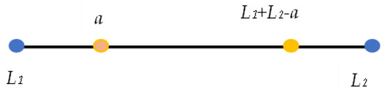
Figure 1.
Reverse point.
In Figure 1, a is any point in the interval [L1, L2], then the reverse point of the vector a is L1 + L2-a. In higher dimensional spaces, points obtained in this way for each dimension are called inverse points. The specific calculation equation follows:
Among them, is the position information of the current individual; represents the position information of the individual after reverse learning; is the minimum value of feasible solutions; is the maximum value of feasible solutions; and is a constant, which is taken as 1 in this paper.
In this paper, the reverse learning mechanism is carried out in stages. Firstly, we sort the population according to the fitness value, and divide the population into three layers. The proportion of the population of each layer is 1:3:6. For the population of the first layer, it can be regarded as being at the top of the pyramid, and its fitness value is better, so the population of this layer will not be reverse-learned. For the population of the second layer, we need to calculate the fitness values of various groups before reverse learning; we then perform reverse learning on the population and calculate the fitness value of various groups after reverse learning. Next we compare the fitness value before improvement with the fitness value after improvement; if the fitness value after improvement is better, the original population is replaced with the improved population; otherwise, we keep the original population. Whether to perform reverse learning is judged according to Equation (14). For the population of the third layer, due to their low fitness value and poor performance, all of them are reverse-learned.
This paper not only applies the reverse learning mechanism in population initialization, but also applies the reverse learning mechanism to the iterative update process of whales.
2.2.3. Dynamically Adjust the Probability Threshold
In WOA, in order to synchronously carry out the process of shrinking and spiraling, the original algorithm sets the probability of selecting both behaviors at 50%. A random number between [0, 1] generated by rand function is compared with the probability threshold, and then the choice is made. The method of setting equal probability thresholds in the original algorithm lacks consideration of changes in population diversity. An adaptive parameter is introduced to replace the original probability threshold. The adaptive probability threshold can be changed in the interval [0, 1] with the iteration of the algorithm, so that the whales have a greater probability to choose a prey strategy suitable for the current group in different periods, thereby coordinating the global search and local development capabilities of the algorithm. The mathematical model of the adaptive probability is shown in Equations (15) and (16), where in Equation (15) is a random number generated by using the Circle chaotic map. Figure 2 shows the change of adaptive probability threshold with the number of iterations.
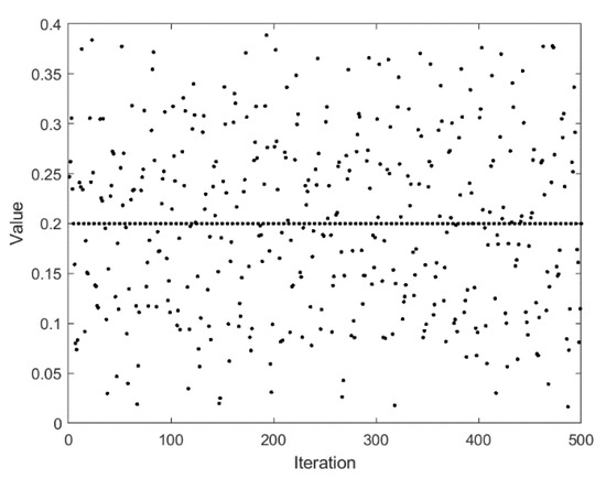
Figure 2.
Variation in the adaptive probability threshold with the number of iterations.
2.2.4. Convergence Factor for Nonlinear Variation
Similar to other algorithms, WOA also has the phenomenon of inconsistency between global search ability and local development ability when solving problems. The convergence factor a has a great influence on parameter A, which is very important for the adjustment of the algorithm’s global search ability and local development ability. In the original algorithm, as the number of iterations increases, the convergence factor decreases linearly from 2 to 0. This linear change in the convergence factor cannot adjust well the global exploration and local development capabilities of the algorithm. In order to make the algorithm maintain the diversity of the population and jump out of the local optimal solution in time, a nonlinearly changing convergence factor is proposed, such as Equation (17).
Figure 3 shows the change in the convergence factor a as the number of iterations increases. It can be seen that compared with the original change method, the improved convergence factor achieves a larger value in the early stage of the iteration, and the value fluctuates within a certain range, which improves the global search ability and enhances randomness.
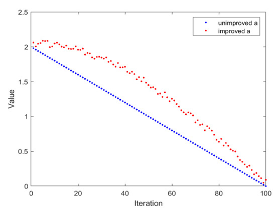
Figure 3.
The variation in convergence factor with the number of iterations.
2.2.5. Adaptive Step Size
In the search phase, the location update is mainly performed according to Equation (9). From this, we can find that the choice of the whale’s next location is affected by three factors: the randomly selected location of the whale and the coefficient vectors A and D. When the coefficient vector , it indicates that the whale is outside the shrinking encirclement, and the whale currently makes a random selection. When the coefficient vector |A| < 1, the whale group keeps shrinking the encircling circle. At the end of the iteration, the value of A becomes increasingly closer to 0, which is detrimental to better updating of the position and limits the local search ability of the algorithm.
For this reason, this paper introduces a new parameter U, which adaptively changes the step size to balance the global search and local search capabilities. It is applied to the position update equation. The evaluation of U is:
where is used to verify symbols. The parameter in has a great influence on the convergence of the algorithm. Through continuous simulation attempts, it is found that when the value of is small, the overall effect of the algorithm is better. The change in k is shown in Figure 4.
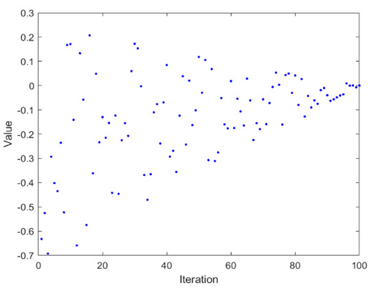
Figure 4.
Effect of the number of iterations on k.
2.2.6. IOWA Implementation Process
In summary, the main implementation process of IWOA proposed in this paper follows. The pseudocode is shown in Figure 5.
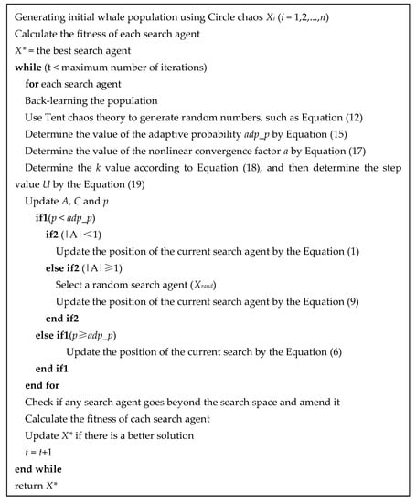
Figure 5.
IWOA implementation pseudocode.
Step 1. Initialize the population. Set the maximum number of iterations Max_iter = 100; population size SearchAgents_no = 30; logarithmic spiral shape constant b = 1.
Step 2. Initialize the population using the Circle chaotic map.
Step 3. Fitness value calculation, looking for individual extreme value and group extreme value.
Step 4. Adopt a reverse learning mechanism for the population.
Step 5. Use Tent chaos theory to generate random numbers, such as Equation (12).
Step 5. Update a according to Equation (17), update k according to Equation (18), update A and C according to Equations (4) and (20).
Step 5. Update the parameter adp_p according to Equation (15).
Step 6. By analyzing the value of the parameter |A| and comparing the size of p and adp_p, the corresponding update scheme is selected: surround prey, bubble net attack, and search for prey.
Step 7. Determine whether the termination condition is met. If it is satisfied, output the optimal solution and position information, otherwise go to Step 3.
3. Performance Test of IWOA
3.1. Test Function and Experimental Environment
In this paper, the proposed algorithm is simulated and experimented based on an AMD Ryzen 7 5800 H CPU, 3.20 GHz main frequency, 16.0 GB memory, and Windows 10 (64 bit) operating system. The programming software is MATLAB 2020a. To verify the performance of the IWOA algorithm, 18 typical benchmark test functions are selected for the test experiments, which are shown in Table 1. In Table 1, F1–F4 denote single-peak functions, which are used to check the local exploitation capability of the algorithm; F5–F9 are complex multipeak functions to evaluate the exploration capability; F10–F18 are fixed-dimensional multipeak functions, which are mainly used to evaluate the algorithm to remove the local optimum.

Table 1.
Details of 18 benchmark functions.
In this paper, the algorithm is tested in three aspects: (1) under the same population size, iteration times, and running times, the convergence speed and solution accuracy of IWOA and WOA, PSO, GSA, DE, and other classical algorithms on different test functions are compared; (2) the effectiveness of different improvement strategies on the optimization performance of WOA is analyzed; and (3) compared with other improved WOAs to verify the effectiveness and competitiveness of the algorithm proposed in this paper.
3.2. Performance Comparison with Classical Intelligent Algorithms
In order to verify the superiority and robustness of the proposed algorithm in solving functions, it is compared with the optimization results of WOA, PSO, GSA, and DE on 18 test functions. We set the population size to 30, the dimension to 30, and the maximum number of iterations to 500.
The test performance of the algorithm is mainly judged according to two criteria: the fitness average AVE and the fitness standard deviation STD. AVE represents the average value of the optimal solution obtained after the algorithm runs independently for many times. The smaller the average value, the better the global search ability of the algorithm and the diversity of the population; its expression is shown in Equation (21).
In Equation (21), represents the number of independent runs, and represents the optimal solution obtained by the r-th test of the algorithm. STD represents the standard deviation of the optimal solution obtained after the algorithm runs independently for many times. The smaller the standard deviation, the better the stability of the algorithm; its expression is shown in Equation (22).
The run was repeated 30 times independently, and the mean and standard deviation of the results of the 30 experiments were taken. The experimental results are shown in Table 2. Table 3 is the result of sorting the algorithms according to the test results of Table 2.
Table 2.
Comparing IWOA with the performance of other algorithms.
Table 3.
Algorithm performance ranking.
When sorting, we first compare the average values of each algorithm on different test functions, and then compare the standard deviation when the average values are the same. The value of ranksum is the sum of performance rankings of each algorithm on different test functions, and rankave is its average value. Finally, the final ranking of each algorithm is obtained according to rankave.
It can be seen from Table 2 and Table 3 that IWOA has the best performance on the 10 benchmark functions. Among them, the theoretical optimal value is obtained when solving 8 functions (F1, F5, F11, F16, F17, F18, F22, F23). Among the 18 tested functions, IWOA ranks the worst only when solving F18. The number of functions that the other four algorithms obtain the optimal solution among the 18 test functions is: 2, 1, 1, and 3. As can be seen from Table 3, IWOA ranks first, followed by DE, GSA, PSO, and WOA. In the unimodal function test, IWOA performs significantly better than the other four algorithms when solving F1 and F2. When solving F3 and F4, although the optimization effect of IWOA is not the best, the ranking of IWOA is in the middle position. In the multimodal function test, IWOA outperformed the other four algorithms when solving F5–F7. When solving F8 and F9, IWOA does not work well, but both mean and standard deviation are better than WOA. When solving the fixed-dimensional multimodal functions F10–F13, F17, and F18, the solution effect of IWOA is obviously better than the other algorithms. When solving F14, the effect of IWOA is slightly weaker than that of PSO and GSA. When solving F15, IWOA is slightly weaker than GSA, but better than other algorithms. When solving F16, IWOA ranks second. Figure 6, Figure 7, Figure 8, Figure 9, Figure 10, Figure 11, Figure 12, Figure 13, Figure 14, Figure 15, Figure 16, Figure 17, Figure 18, Figure 19, Figure 20, Figure 21, Figure 22 and Figure 23 show the convergence of five algorithms on 18 test functions.
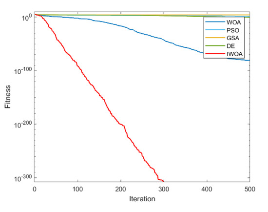
Figure 6.
F1.
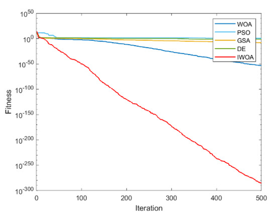
Figure 7.
F2.
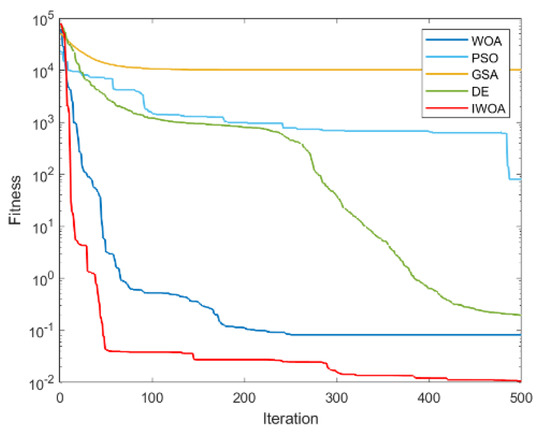
Figure 8.
F3.
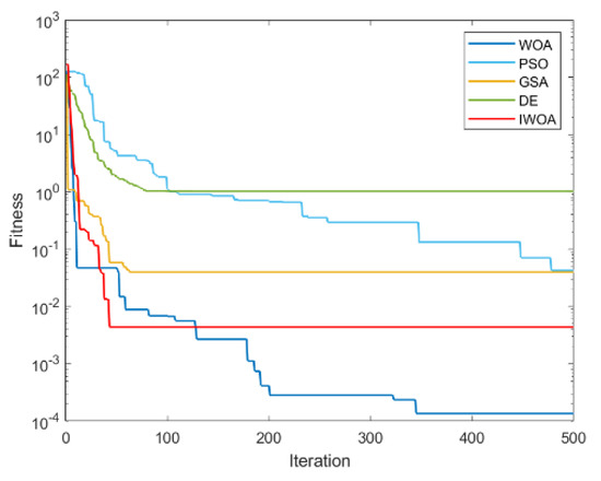
Figure 9.
F4.
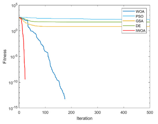
Figure 10.
F5.
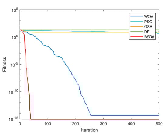
Figure 11.
F6.
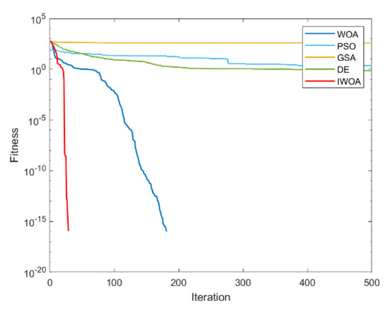
Figure 12.
F7.
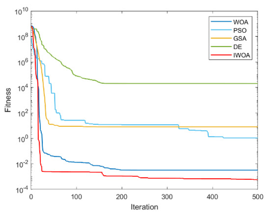
Figure 13.
F8.
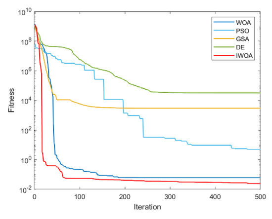
Figure 14.
F9.
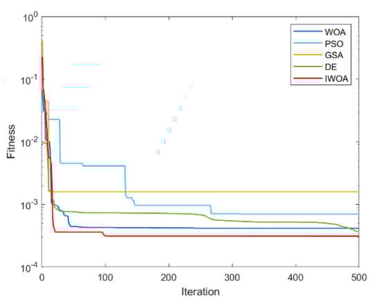
Figure 15.
F10.
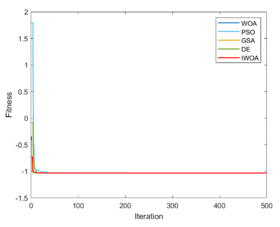
Figure 16.
F11.
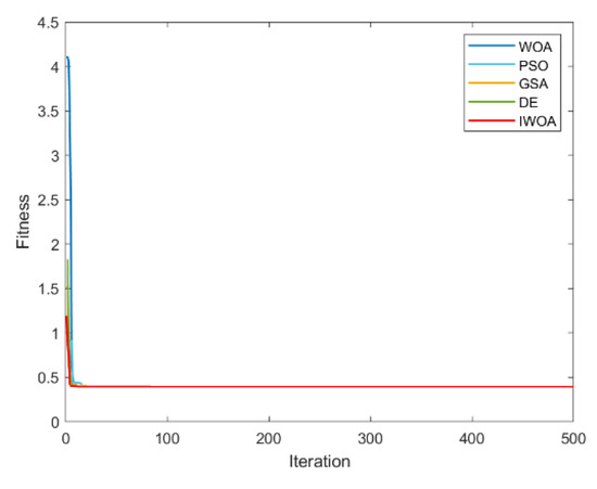
Figure 17.
F12.
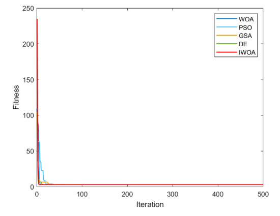
Figure 18.
F13.
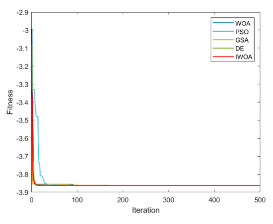
Figure 19.
F14.
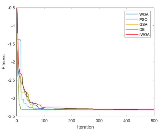
Figure 20.
F15.
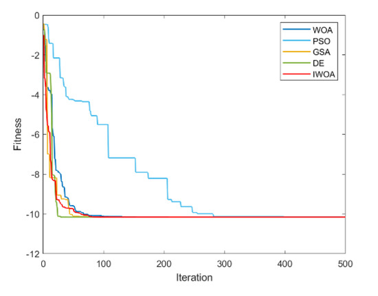
Figure 21.
F16.
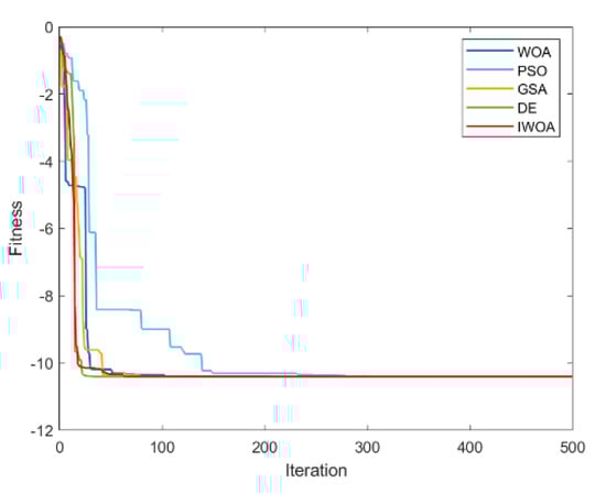
Figure 22.
F17.
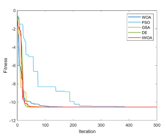
Figure 23.
F18.
3.3. Effect of Improving the Strategy on the Performance of the Algorithm
To analyze the influence of different improvement strategies on the optimization performance of the standard WOA algorithm, IWOA is compared with RLWOA (WOA algorithm with only reverse learning mechanism), DTWOA (WOA algorithm with only dynamic threshold), NCFWOA (WOA algorithm with only nonlinear convergence factor), and CMWOA (WOA algorithm with only chaotic mapping). The parameter settings of the four algorithms are the same as those in the previous section. The test results are shown in Table 4.
Table 4.
Influence of different improvement strategies on WOA performance.
It can be seen from Table 4 that the improvement strategy for the dynamic threshold and nonlinear convergence factor has limited contribution to the improvement of WOA performance. However, its performance in solving a few functions is still very good. For example, NCFWOA performs somewhat better than IWOA in solving F7 and F12. The improved strategy of chaotic mapping and reverse learning mechanism has played a positive role in improving the performance of WOA. On the whole, there is still a big gap between the overall performance of the algorithm and IWOA by using only one improved strategy. By absorbing the advantages of various improvement strategies, IWOA converges faster when testing functions. Additionally, for most of the test functions, the solution accuracy and optimization results are better than other algorithms.
3.4. Performance Comparison with Other Improved Whale Optimization Algorithms
In order to compare the optimization performance of the algorithm proposed in this paper with other improved WOAs, the data in references [42,43] are cited for comparative experiments. We set the population size to 30, set the maximum number of iterations to 500, and ran the test 30 times independently. The performance of the algorithm is tested by comparing the average and standard deviation of the test results. The specific results are shown in Table 5. It can be seen from Table 5 that, except for F20, IWOA performs better than the other two algorithms when solving other functions. When solving F20, however, the performance of IWOA is weaker than that of ESWOA and HWGO. Additionally, in nine test functions, IWOA obtained the optimal value when solving five of them, which is much better than the other two algorithms.
Table 5.
Performance comparison for IWOA and other improved WOAs.
4. Algorithm Application Analysis Algorithm
To test the optimization performance of the algorithm in solving practical problems, in this section, the convergence speed and solution accuracy of IWOA in solving the charging station location optimization model considering the cost problem are studied.
4.1. Optimal Model of Charging Station Site Selection
With the enhancement of people’s awareness of environmental protection, energy saving and environmental protection have become important considerations for consumers when purchasing automobiles [44,45]. The continuous increase in the number of new-energy vehicles has driven the development of industries such as charging infrastructure. Reasonable charging station site selection has important strategic significance for the development of electric vehicles. In the process of establishing the site selection model, this paper mainly considers the interests of two aspects: enterprises and users. It is necessary to ensure that the company is profitable, and to reduce the cost of charging users as much as possible. Generally speaking, the location model is a nonlinear programming model with complex constraints, which belongs to an NP-hard problem.
When establishing the location model, this paper draws on the ideas of the traditional P-median model [46] and the maximum coverage model [47]. Under the premise of satisfying the constraints, a site selection model with the goal of minimizing the comprehensive cost is established and strives to make the charging service range fully covered in the study area. The objective function of the location optimization model is shown in Equation (23), which consists of three parts: annual construction and operation cost , time cost , and penalty term .
mainly consists of two parts, including the construction cost and the operating cost , the mathematical expression is provided as Equation (24). Among them, mainly includes charging pile, land, transformer, and other costs, as shown in Equation (25); mainly includes labor cost and equipment maintenance cost, as shown in Equation (26). Equation (27) is the annual time-consuming cost. Equation (28) is a constraint in the location model, and it can be found from the formula that it mainly includes two parts. The first part is that the distance between two charging service stations should be no less than 6 km. The reason for this setting is that the distance between some charging stations is too close at present, resulting in excessive concentration of charging resources. Ca is the number of service stations that do not meet the 6 km constraint. The second part of Equation (28) is the constraint on the service capacity of the charging station. The station selected as the charging service station needs to be able to provide charging service for the vehicles coming to charge. Because of the different number of charging piles in each charging station, it is difficult for some stations to meet the charging demand of electric vehicles at times during the peak charging period. Cc is the number of charging stations that cannot meet the charging demand at this point. On the one hand, these two parts in Equation (28) are to balance the charging resources and improve the charging convenience of users; on the other hand, it can improve the overall utilization rate of charging service stations and protect the interests of enterprises.
In Equations (23)–(28), is the set of charging service stations, and is the charging station; is the discount rate, = 0.08; is the depreciation period, = 20 years; is the fixed investment cost, this paper sets the cost of a charging station to be 1 million CNY; is the number of charging piles in the station; is the equivalent investment coefficient of related equipment costs and its value is 10,000 CNY/unit2; is the unit price of the charging pile. In this paper, the price of a single charging pile is set at 100,000 CNY; is the conversion factor of labor and equipment operation and maintenance costs, = 0.1; is the distance from each charging demand point to the charging service station that provides services for it; is the amount spent by the electric vehicle per kilometer, and its value is 1.79 CNY.
In addition to the two constraints mentioned in the penalty item, the setting of constraints also needs to consider the demand distribution relationship and coverage.
Each charging demand point can only be served by one charging service station, such as Equation (29). Equation (30) specifies that the number of charging service stations is . Equation (31) ensures that the demand at the demand point can only be provided by the charging service station. In Equation (32), and take the value 0 or 1. represents the service demand distribution relationship between the charging demand point and the charging service station.
In Equations (29)–(32), is the set of all demand points and is the charging demand point. When the value of is 1, it means that the demand of charging demand point is provided by charging service station , otherwise it is 0. When the value of is 1, it means that point is selected as the charging service station.
4.2. Using IWOA to Solve the Charging Station Location Model
To verify the effectiveness of IWOA in solving the location optimization problem, IWOA and WOA were used to solve the location model. In this case, there are a total of 130 charging stations. The number of sites varies from 12 to 24. The number of iterations is 100.
To better analyze the impact of changes in the number of sites on the site selection scheme, this paper sets the minimum number of sites as 12 and the maximum number of sites as 24. It can be found from Table 6 that when the number of charging stations is 23, the minimum annual construction and operation cost can be solved. When the number of charging stations is 24 and 13, the minimum time cost and penalty value, respectively, can be obtained. The costs are sorted in order from small to large. When the number of charging stations is 14, the scheme ranks 1st in comprehensive cost, 6th in annual construction and operation cost, 13th in time cost, and 4th in penalty. Overall, when 14 charging stations are installed, the comprehensive cost is the smallest.
Table 6.
Costs for different number of sites.
According to Table 6, we determined that the number of charging service stations is 14. To verify the effectiveness of the algorithm improvement, we use IWOA and WOA to solve the location model. Table 7 shows the comparison of various elements when using IWOA and WOA to solve the location problem. As can be seen from Table 7, the comprehensive cost obtained by IWOA is 128,131.9 less than WOA. Except for , IWOA performs better than WOA in terms of , , and convergence speed.
Table 7.
Performance comparison for IWOA and other improved WOAs.
Figure 24 shows the convergence curves of the two algorithms for solving the same location model. As can be seen from the figure, the IWOA algorithm is far better than IWOA in terms of convergence speed and solution accuracy. Figure 25 shows the site selection results obtained by using the IWOA algorithm. The red squares in the figure are charging service stations, and the green dots are charging demand stations.
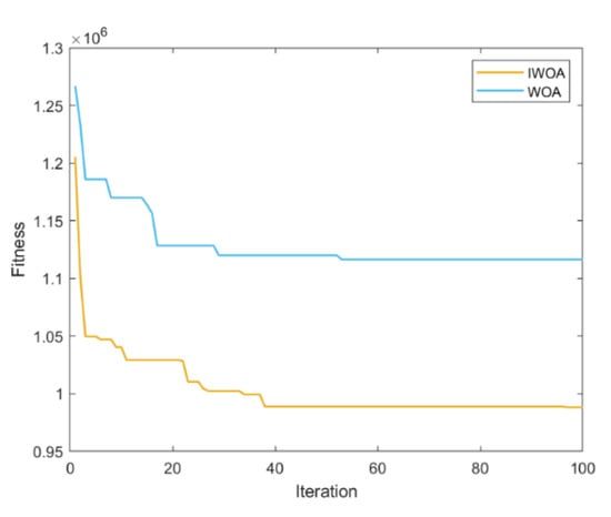
Figure 24.
Convergence curve.
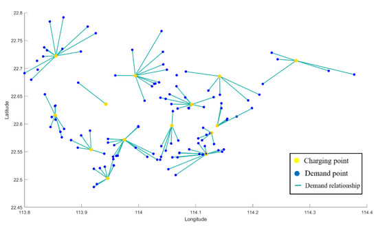
Figure 25.
Optimization results of charging station site selection.
The Voronoi diagram has the following characteristics: there is one generator in each V polygon; the distance from each V polygon to the generator is shorter than the distance to other generators; the distance between the points on the polygon boundary and the generator that generates the boundary is equal. We use these features of the Voronoi diagram to divide the service range of charging stations. Figure 26 shows the division result of the service range of the charging station. The blue dots in Figure 26 are charging service stations, the red star points are charging demand stations, and the blue borders are charging range boundaries.
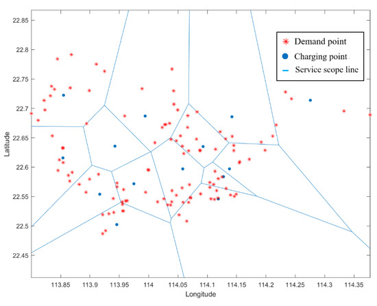
Figure 26.
Using a Voronoi diagram to divide the service scope of charging stations.
5. Conclusions
This paper proposes an improved whale optimization algorithm based on hybrid strategy and applies it to the location optimization problem of electric vehicle charging stations. Finally, the following conclusions are drawn:
- The optimization performance of the IWOA algorithm is significantly improved. In the performance test of 18 benchmark functions, the overall performance of IWOA is better than that of DE, GSA, PSO, and WOA. Compared with the traditional multiobjective optimization-improved whale algorithm, IWOA has better global optimization ability and solution speed.
- The addition of chaotic mapping and reverse learning mechanism provides an important contribution to the performance improvement of the algorithm. The improvement of the algorithm performance by adopting the hybrid strategy is stronger than that of the single improvement strategy.
- The overall cost is the smallest when the number of charging stations is set to 14. When using IWOA and WOA to solve the model, the solution accuracy and convergence speed of IWOA are better than those of WOA.
This paper enriches the research on locating electric vehicle charging stations, and provides a feasible scheme for the location of electric vehicle charging stations, which has important practical value. However, there are still further needs in the current research, such as the performance of the improved whale optimization algorithm in solving higher-dimensional and more complex problems, the location model considering various factors, among others. In the future, many measures can be tried to improve the whale optimization algorithm, to increase the convergence speed and solution accuracy of the whale optimization algorithm. At the same time, there are more factors that can be taken into account when establishing the site selection model. These include the uncertainty of demand, the impact of site selection on carbon emissions, the connection between charging station and power grid, etc.
Author Contributions
Conceptualization, Y.L., W.P. and Q.Z.; methodology, Y.L. and W.P.; software, Y.L.; validation, Y.L., W.P. and Q.Z.; formal analysis, Y.L., W.P. and Q.Z.; investigation, Y.L. and W.P.; resources, Y.L.; data curation, Y.L., W.P. and Q.Z.; writing—original draft preparation, Y.L.; writing—review and editing, W.P. and Q.Z.; visualization, Y.L. and W.P.; supervision, W.P. and Q.Z.; project administration, W.P. and Q.Z.; funding acquisition, W.P. and Q.Z. All authors have read and agreed to the published version of the manuscript.
Funding
This research was funded by Shandong Provincial Natural Science Foundation, grant number ZR2020QF059, ZR2021MF131; Foundation of State Key Laboratory of Automotive Simulation and Control, grant number 20181119; National Natural Science Foundation of China (62203271).
Institutional Review Board Statement
Not applicable.
Informed Consent Statement
Not applicable.
Data Availability Statement
Not applicable.
Acknowledgments
The authors would like to thank the anonymous reviewers and the Editor for their helpful comments.
Conflicts of Interest
The authors declare no conflict of interest.
References
- Yi, T.; Zhang, C.; Lin, T.; Liu, J. Research on the spatial-temporal distribution of electric vehicle charging load demand: A case study in China. J. Clean. Prod. 2020, 242, 118457.1–118457.15. [Google Scholar] [CrossRef]
- Pei, W.; Zhang, Q.; Li, Y. Efficiency Optimization Strategy of Permanent Magnet Synchronous Motor for Electric Vehicles Based on Energy Balance. Symmetry 2022, 14, 164. [Google Scholar] [CrossRef]
- Zong, G.; Wang, Y.; Karimi, H.; Shi, K. Observer-based adaptive neural tracking control for a class of nonlinear systems with prescribed performance and input dead-zone constraints. Neural Netw. 2022, 147, 126–135. [Google Scholar] [CrossRef] [PubMed]
- Wang, Y.; Zong, G.; Yang, D.; Shi, K. Finite-time adaptive tracking control for a class of nonstrict feedback nonlinear systems with full state constraints. Int. J. Robust Nonlinear Control 2022, 32, 2551–2569. [Google Scholar] [CrossRef]
- Sun, H.; Zong, G.; Cui, J.; Shi, K. Fixed-time sliding mode output feedback tracking control for autonomous underwater vehicle with prescribed performance constraint. Ocean. Eng. 2022, 247, 110673:1–110673:10. [Google Scholar] [CrossRef]
- Ai, Z.; Peng, L.; Zong, G.; Shi, K. Impulsive control for nonlinear systems under dos attacks: A dynamic event-triggered method. IEEE Trans. Circuits Syst. II Express Briefs 2022, 69, 3839–3843. [Google Scholar] [CrossRef]
- Yang, S.; Zhang, D.; Fu, J.; Fan, S.; Ji, Y. Market Cultivation of Electric Vehicles in China: A Survey Based on Consumer Behavior. Sustainability 2018, 10, 4056. [Google Scholar] [CrossRef]
- Wu, J.; Liao, H.; Wang, J. Analysis of consumer attitudes towards autonomous, connected, and electric vehicles: A survey in China. Res. Transp. Econ. 2020, 80, 100828. [Google Scholar] [CrossRef]
- Cao, W.; Wan, Y.; Wang, L.; Wu, Y. Location and capacity determination of charging station based on electric vehicle charging behavior analysis. IEEJ Trans. Electr. Electron. Eng. 2021, 16, 827–834. [Google Scholar] [CrossRef]
- Li, Y.; Pei, W.; Xu, D. Electric Vehicle Charging Station Planning Based on Immune Algorithm and Voronoi Diagram. In Proceedings of the 2021 40th Chinese Control Conference (CCC), Shanghai, China, 26–28 July 2021; pp. 1532–1537. [Google Scholar] [CrossRef]
- Xu, D.; Pei, W.; Li, Y. Location Selection of Electric Vehicle Charging Station Based on Improved Immune Algorithm. In Proceedings of the 2021 40th Chinese Control Conference (CCC), Shanghai, China, 26–28 July 2021; pp. 1538–1543. [Google Scholar] [CrossRef]
- Xu, D.; Pei, W.; Zhang, Q. Optimal Planning of Electric Vehicle Charging Stations Considering User Satisfaction and Charging Convenience. Energies 2022, 15, 5027. [Google Scholar] [CrossRef]
- Hu, L.; Dong, J.; Lin, Z.; Yang, J. Analyzing battery electric vehicle feasibility from taxi travel patterns: The case study of New York City, USA. Transp. Res. Part C 2018, 87, 91–104. [Google Scholar] [CrossRef]
- Li, Y.; Pei, W. Three-stage location optimization decision of charging station based on multi-source data. Control Eng. China 2022, 1–10. [Google Scholar] [CrossRef]
- Zeng, B.; Dong, H.; Sioshansi, R.; Xu, F.; Zeng, M. Bi-Level Robust Optimization of Electric Vehicle Charging Stations with Distributed Energy Resources. IEEE Trans. Ind. Appl. 2020, 56, 5836–5847. [Google Scholar] [CrossRef]
- Wang, X.; Wang, J.; Huang, S.; Lv, X. Research on Location of Charging Station of Electric Vehicle Based on Improved TLBO. J. Phys. Conf. Ser. 2020, 1676, 012188. [Google Scholar] [CrossRef]
- Islam, T.; Islam, M.; Ruhin, M. An analysis of foraging and echolocation behavior of swarm intelligence algorithms in optimization: ACO, BCO and BA. Int. J. Intell. Sci. 2018, 8, 1. [Google Scholar] [CrossRef][Green Version]
- Xue, J.; Shen, B. A novel swarm intelligence optimization approach: Sparrow search algorithm. Syst. Sci. Control Eng. 2020, 8, 22–34. [Google Scholar] [CrossRef]
- Tharwat, A.; Elhoseny, M.; Hassanien, A.; Gabel, T.; Kumar, A. Intelligent Bézier curve-based path planning model using Chaotic Particle Swarm Optimization algorithm. Clust. Comput. 2019, 22, 1–22. [Google Scholar] [CrossRef]
- Gong, G.; Chiong, R.; Deng, Q.; Gong, X. A hybrid artificial bee colony algorithm for flexible job shop scheduling with worker flexibility. Int. J. Prod. Res. 2020, 58, 4406–4420. [Google Scholar] [CrossRef]
- Zhao, J.; Liu, S.; Zhou, M.; Guo, X.; Qi, L. Modified Cuckoo Search Algorithm to Solve Economic Power Dispatch Optimization Problems. IEEE/CAA J. Autom. Sin. 2018, 5, 794–806. [Google Scholar] [CrossRef]
- Jagatheesan, K.; Anand, B.; Samanta, S.; Dey, N.; Ashour, A.; Balas, V. Design of a proportional-integral-derivative controller for an automatic generation control of multi-area power thermal systems using firefly algorithm. IEEE/CAA J. Autom. Sin. 2019, 6, 503–515. [Google Scholar] [CrossRef]
- Qiao, W.; Yang, Z.; Kang, Z.; Pan, Z. Short-term natural gas consumption prediction based on Volterra adaptive filter and improved whale optimization algorithm. Eng. Appl. Artif. Intell. 2020, 87, 103323. [Google Scholar] [CrossRef]
- Emadedin, H.; Madjid, T.; Maryam, B. A New Particle Swarm Optimization Algorithm for Optimizing Big Data Clustering. SN Comput. Sci. 2022, 3, 311. [Google Scholar] [CrossRef]
- Karaboga, D.; Basturk, B. A powerful and efficient algorithm for numerical function optimization: Artificial bee colony (ABC) algorithm. J. Glob. Optim. 2007, 39, 459–471. [Google Scholar] [CrossRef]
- Rashedi, E.; Nezamabadi-pour, H.; Saryazdi, S. GSA: A Gravitational Search Algorithm. Inf. Sci. 2009, 179, 2232–2248. [Google Scholar] [CrossRef]
- Storn, R.; Price, K. Differential Evolution—A Simple and Efficient Heuristic for global Optimization over Continuous Spaces. J. Glob. Optim. 1997, 11, 341–359. [Google Scholar] [CrossRef]
- Deng, W.; Shang, S.; Cai, X.; Zhao, H.; Zhou, Y.; Chen, H.; Deng, W. Quantum differential evolution with cooperative coevolution framework and hybrid mutation strategy for large scale optimization. Knowl.-Based Syst. 2021, 224, 107080. [Google Scholar] [CrossRef]
- Wei, D. Network traffic prediction based on RBF neural network optimized by improved gravitation search algorithm. Neural Comput. Appl. 2017, 28, 2303–2312. [Google Scholar] [CrossRef]
- Chegini, S.; Bagheri, A.; Najafi, F. PSOSCALF: A new hybrid PSO based on Sine Cosine Algorithm and Levy flight for solving optimization problems. Appl. Soft Comput. J. 2018, 73, 697–726. [Google Scholar] [CrossRef]
- Mirjalili, S.; Lewis, A. The Whale Optimization Algorithm. Adv. Eng. Softw. 2016, 95, 51–67. [Google Scholar] [CrossRef]
- Fan, Q.; Chen, Z.; Li, Z.; Xia, Z.; Yu, J.; Wang, D. A new improved whale optimization algorithm with joint search mechanisms for high-dimensional global optimization problems. Eng. Comput. 2020, 37, 1851–1878. [Google Scholar] [CrossRef]
- Ning, G.; Cao, D. Improved Whale Optimization Algorithm for Solving Constrained Optimization Problems. Discret. Dyn. Nat. Soc. 2021, 2021, 8832251. [Google Scholar] [CrossRef]
- Bozorgi, S.; Yazdani, S. IWOA: An improved whale optimization algorithm for optimization problems. J. Comput. Des. Eng. 2019, 6, 243–259. [Google Scholar] [CrossRef]
- Ling, Y.; Zhou, Y.; Luo, Q. Lévy Flight Trajectory-Based Whale Optimization Algorithm for Global Optimization. IEEE Access 2017, 5, 6168–6186. [Google Scholar] [CrossRef]
- Sun, G.; Shang, Y.; Zhang, R. An Efficient and Robust Improved Whale Optimization Algorithm for Large Scale Global Optimization Problems. Electronics 2022, 11, 1475. [Google Scholar] [CrossRef]
- Yan, Z.; Sha, J.; Liu, B.; Tian, W.; Lu, J. An Ameliorative Whale Optimization Algorithm for Multi-Objective Optimal Allocation of Water Resources in Handan, China. Water 2018, 10, 87. [Google Scholar] [CrossRef]
- Provas, R.; Chandan, P.; Vivekananda, M. Optimal Solution of Combined Heat and Power Dispatch Problem Using Whale Optimization Algorithm. Int. J. Appl. Metaheuristic Comput. 2021, 13, 1–26. [Google Scholar] [CrossRef]
- Zhang, H.; Tang, L.; Yang, C.; Lan, S. Locating electric vehicle charging stations with service capacity using the improved whale optimization algorithm. Adv. Eng. Inform. 2019, 41, 100901. [Google Scholar] [CrossRef]
- Cheng, J.; Xu, J.; Chen, W.; Song, B. Locating and sizing method of electric vehicle charging station based on Improved Whale Optimization Algorithm. Energy Rep. 2022, 8, 4386–4400. [Google Scholar] [CrossRef]
- Zhu, H.; Tong, X.; Wang, Z.; Ma, J. A novel method of dynamic S-box design based on combined chaotic map and fitness function. Multimed. Tools Appl. 2020, 79, 12329–12347. [Google Scholar] [CrossRef]
- Kumar, G.; Jatoth, C.; Gangadharan, G.; Buyya, R. QoS-aware cloud service composition using eagle strategy. Future Gener. Comput. Syst. 2019, 90, 273–290. [Google Scholar] [CrossRef]
- Korashy, A.; Kamel, S.; Jurado, F.; Youssef, A. Hybrid Whale Optimization Algorithm and Grey Wolf Optimizer Algorithm for Optimal Coordination of Direction Overcurrent Relays. Electr. Power Compon. Syst. 2019, 47, 1–15. [Google Scholar] [CrossRef]
- Ji, Z.; Huang, X. Plug-in electric vehicle charging infrastructure deployment of China towards 2020: Policies, methodologies, and challenges. Renew. Sustain. Energy Rev. 2018, 90, 710–727. [Google Scholar] [CrossRef]
- Du, J.; Ouyang, M.; Chen, J. Prospects for Chinese electric vehicle technologies in 2016–2020: Ambition and rationality. Energy 2016, 120, 584–596. [Google Scholar] [CrossRef]
- Abdulkader, M.; Fazlay, F.; Ammar, N.; Alok, T. Using the location-allocation P-median model for optimising locations for health care centres in the city of Jeddah City, Saudi Arabia. Geospat. Health 2021, 16. [Google Scholar] [CrossRef]
- Richard, M.; Ricardo, H.; Sebastián, R. Optimal location of bike-sharing stations: A built environment and accessibility approach. Transp. Res. Part A 2022, 160, 126–142. [Google Scholar] [CrossRef]


Publisher’s Note: MDPI stays neutral with regard to jurisdictional claims in published maps and institutional affiliations. |
© 2022 by the authors. Licensee MDPI, Basel, Switzerland. This article is an open access article distributed under the terms and conditions of the Creative Commons Attribution (CC BY) license (https://creativecommons.org/licenses/by/4.0/).