A 1D-3D Coupling Model to Evaluate Hydropower Generation System Stability

Abstract

This paper proposes a novel 1D-3D approach for the stability characteristics of the hydropower generation system (HGS) in transition processes. First, a 1D-3D coupling model was established for the HGS in the load-reduction process. Second, a sensitivity analysis of the HGS’s parameters to the rotation speed and discharge was conducted. Third, the pressure pulsation characteristics of the HGS with three typical guide vane openings were analyzed during the load-reduction process. The results show that with the closure of the guide vane, the discharge gradually decreases and it is sensitive to the change in hydraulic parameters. The rotation speed fluctuates at the early stage of the transition process and is easily affected by mechanical parameters. In addition, the pressure pulsation inside the Francis turbine is more intense under small openings than large openings, and the primary frequency of pressure pulsation under three opening degrees is the blade frequency. The 1D-3D coupling model successfully integrates the advantages of traditional methods and provides a reference for predicting system stability and exploring the stability mechanism.

1. Introduction

The hydropower generation system (HGS) is playing an increasingly important role in the world’s energy applications [1,2]. The rapid growth of intermittent energy sources, such as wind power and photovoltaic, has changed the world’s energy structure [3,4]. Therefore, as the proportion of hydropower units increases, the hydropower station is shifting from traditional power generation to peak load and frequency regulation. Due to the intermittent characteristics of wind power and photoelectric power, the requirements of real-time balance of electric energy in the power system cannot be satisfied. With rapid start–stop characteristics of changing load, the hydropower generation system has therefore become the best choice for complementary energy [5,6].

The HGS has received a lot of attention in recent years. There are some risks in the quality of the power grid due to the randomness and unpredictability of intermittent energy [7,8,9]. To keep the balance between active power and reactive power in the power grid, a higher requirement is put forward for the flexible operation of HGS. Moreover, the stability problem caused by the flexible operation and operation switching has also become a research hotspot. In the transition process of the HGS, the hydraulic–mechanical–electrical subsystem shows a cooperative variation relationship [10]. However, due to the difference in the response time to flow, the machinery, and electricity, the hysteresis appears in a cooperative variation relationship, causing energy fluctuations across the whole system [11]. In addition, the energy fluctuation of the HGS is particularly obvious when the operation switching time is long. The excessive energy fluctuation behavior under the transition process (short time, large scale) not only affects the performance of hydropower but also undoubtedly reduces the service life of the HGS [12,13].

The stability of the HGS in the transition process is a hot issue in many fields, such as the design and operation of hydraulic machinery. It is divided into two kinds of research. First, based on the theory of computational fluid dynamics, the stability mechanism is revealed by observing the internal flow field behavior of the hydroturbine [14,15]. For example, Simon Pasche et al. investigated the birth and the growth of the synchronous pressure wave in Francis turbines, which brought deeper comprehension of the synchronous wave generation mechanism [16]. Zhou et al. used baffles in the draft tube to hinder the swirling flow emerging from a Francis turbine runner during part-load operation [17]. Zhou et al. found the pressure fluctuation in the vaneless zone. The finding is of great significance in terms of understanding the influence of the clearance flow on the load rejection process [18]. The unsteady behavior of the Francis turbine at several operating points was simulated by Ahmed Laouari [19]. The results showed that the strong pressure pulsation and torque oscillations occurred even at the best efficiency operating point. Various studies [20,21,22,23,24] also verified the feasibility of pressure pulsation and velocity distribution of an ultra-high head turbine in a hydropower station under rated and part-load operation. Second, the whole HGS model was established, and the stability law was investigated by combining mathematics and dynamics theory. Guo et al. investigated system stability considering the coupling effect of water potential energy in the surge tank and power grid [25]. Xu et al. established the Hamiltonian model of the HGS with a multi-hydroturbine, and the stability was simulated by introducing several kinds of disturbance [26]. Li identified the fast–slow behavior of the hydropower generation system, which caused the system energy fluctuation [27].

The method of 1D and 3D coupling modeling has been applied in many fields. David et al. discussed several different physical application models, based on the Newton-based method, and adopted the coupling strategy from the loosely coupled Gauss–Seidel and operator splitting methods to the tightly coupled method, achieving a breakthrough in the understanding of coupling problem progress [28]. Zhang et al. studied the performance of neutron and thermal-liquid coupling algorithms in transient problems. Three methods, including operator splitting semi-implicit (OSSI), Picard iteration (PI), and Jacobi-Free Newton–Krylov (JFNK), were used for comparison. The results show that the improved PI and JFNK coupling algorithm can achieve better computing performance in TINTE due to its better accuracy and stability [29]. Peng et al. used the OpenMC software coupled with the commercial computational fluid dynamics of ANSYS. The realization and parallel performance of the PI algorithm of grouped Gauss–Seidel type and grouped Jacobi type were studied. The results show that the adaptive load balancing algorithm can improve the computational efficiency of the block Jacobi algorithm and the performance of the Gauss–Seidel algorithm [30]. Cheng et al. simulated the whole process of water flow and reconnection for the pumped storage system, and showed that the two high-amplitude single pulses generated by the axial force and radial force of the flow channel during this process are destructive [31]. Liu et al. simulated the extreme case of simultaneous load shedding in a prototype pumped storage system. The results show that the maximum pressure is caused by strong static and dynamic interference (RSI), and the maximum pressure upstream of the runner exceeds the industry standard [32]. The application of the two aforementioned methods enriches the stability theories in transition processes. However, both methods have their limitations: (1) The systematic model can only idealize the dynamic process for a long time, which cannot be accurately solved due to the inability of fluid characteristics; (2) due to the complexity of the system, the internal properties cannot be used for calculation; (3) the transition process of the HGS involves collaborative changes in multiple subsystems, and the internal characteristic method cannot meet the requirements of collaborative changes for the subsystems of the HGS.

Motivated by the above analysis, the stability of the HGS was studied during the load-reduction process. Three innovations appear in this paper. First, the synergic model is innovatively introduced, which combines the advantages of system modeling and inner characteristic modeling. Second, the sensitivity of different subsystem parameters to the system output is determined during load-decreasing process. Third, the pressure pulsation inside the hydroturbine under three typical guide vane openings was obtained from a transient perspective.

This paper is organized as follows: Section 2 introduces the synergic system model. Section 3 presents the dynamic behavior and the pressure pulsation under different turbine locations. Section 4 provides the conclusions.

2. The Internal Characteristic Model of the Hydropower Generation System

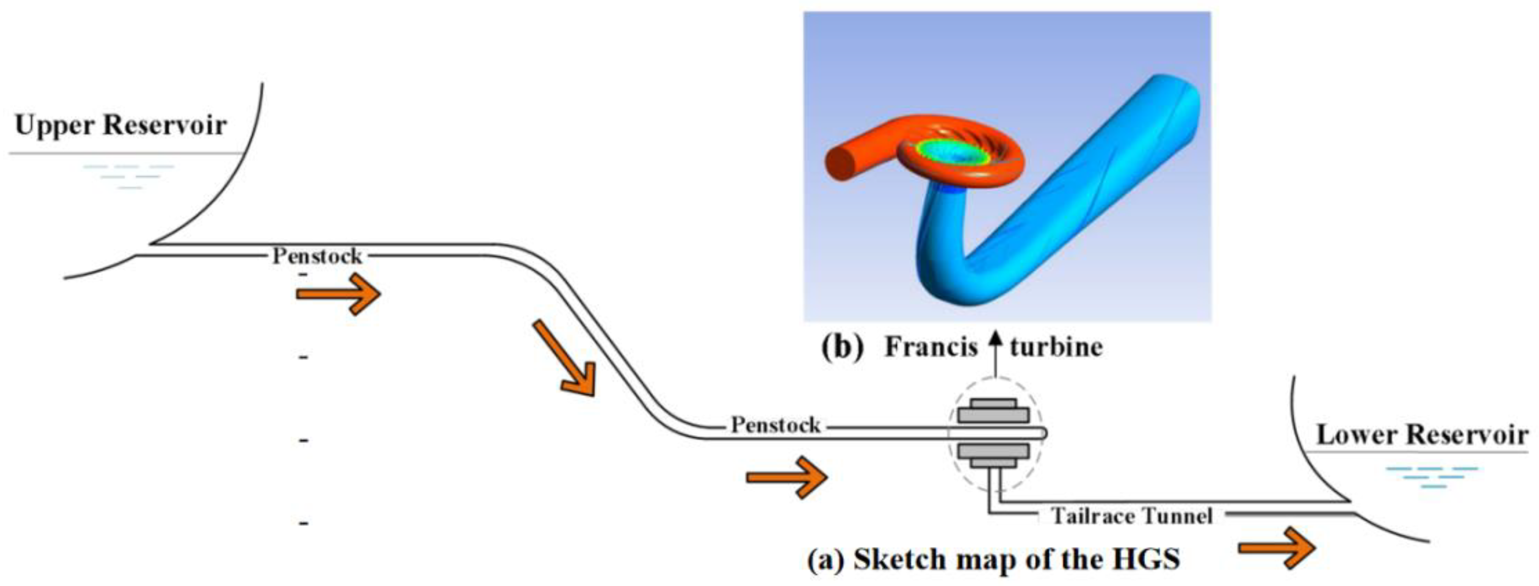
Figure 1a is the sketch map of the HGS. Figure 1b is the inner flow field diagram of the turbine. Traditional systematic modeling was used to model each subsystem separately to study the characteristics of the HGS. The dynamic behavior of subsystems (generators, pressure pipe, penstock, Francis turbine generator, and tailrace tunnel) are easy to describe with ordinary differential equations (ODEs). However, as the energy transformation hub of the HGS, the complexity of the Francis turbine structure creates the turbulent characteristics of flow, which cannot be described using ODEs. Therefore, with systematic modeling, it is difficult to express the transient flow characteristics in the Francis turbine. Compared with systematical modeling, internal characteristic modeling focuses on the refined modeling of a single Francis turbine subsystem, as shown in Figure 1b. The application of the turbulence equation describes the characteristics of the fluid in a more detailed and accurate way, and reveals the unstable mechanism of the unit more intuitively. However, the main drawback or barrier to the internal characteristic modeling method is the reduction process of computing resources and data, which will remain difficult to resolve for the foreseeable future. Combining the advantages of the two approaches, Section 2 establishes the 1D-3D coupling model of the HGS.

2.1. Hydroturbine Model

As the hub of the energy conversion of the HGS, the turbine converts kinetic energy of flow into mechanical energy. The classical hydroturbine model adopts the hydroturbine torque and flow as output, which is expressed as

$$\left\{\begin{array}{l}{M}_t=M_t(H,n,a)\\ Q=Q(H,n,a)\end{array}\right.,$$

(1)

where M_t is the active torque of hydroturbine, and Q is the flow of hydroturbine inlet. Both torque and flow are the function of the water head H of the turbine inlet, rotation speed n, and guide vane opening a.

Expand Equation (1) in an arbitrary operational state using Taylor theory. Therefore, the limitation increment of torque and flow are

$$\begin{array}{l}\Delta M_t=\frac{\partial M_t}{\partial a}\Delta a+\frac{\partial M_t}{\partial n}\Delta n+\frac{\partial M_t}{\partial H}\Delta H\\ \Delta Q=\frac{\partial Q}{\partial a}\Delta a+\frac{\partial Q}{\partial n}\Delta n+\frac{\partial Q}{\partial H}\Delta H\end{array}$$

(2)

The essence of Equation (2) means the variance of output (M_t and Q) equals the sum of the variance of input (a, n, and H) under their direction.

2.1.1. External Characteristic Method of the Turbine

In the external characteristic method, the full characteristic curve of the hydroturbine is regarded as the boundary condition for calculating the long transition process of the HGS. In this paper, the model of the Francis turbine came from a hydraulic machinery experiment platform in Norway [33].

From Equation (2), the partial derivative represents the direction differential. The differential form of Equation (2) is transformed as follows:

$$\begin{array}{l}\stackrel{·}{M_t}=\frac{\partial M_t}{\partial a}\stackrel{·}{a}+\frac{\partial M_t}{\partial n}\stackrel{·}{n}+\frac{\partial M_t}{\partial H}\stackrel{·}{H}\\ \stackrel{·}{Q}=\frac{\partial Q}{\partial a}\stackrel{·}{a}+\frac{\partial Q}{\partial n}\stackrel{·}{n}+\frac{\partial Q}{\partial H}\stackrel{·}{H}\end{array}$$

(3)

The calculation step for six coefficients ($\frac{\partial M_t}{\partial a},\frac{\partial M_t}{\partial n},\frac{\partial M_t}{\partial H},\frac{\partial Q}{\partial a},\frac{\partial Q}{\partial n}$ and $\frac{\partial Q}{\partial H}$) with partial derivative form are obtained in [34].

2.1.2. Pressure Pipe

In the actual design of a hydropower station, the assumption of the elasticity of the pipe wall causes a big error. Therefore, the pressure pipe model, which considers the elastic water hammer and pipe friction, is as follows [35]:

$$\stackrel{⃛}{q}+\frac{24}{T_r^2}\dot{q}+\frac{96f}{T_r^3}q=-\frac{3}{h_w{T}_r}\ddot{h}-\frac{12f}{h_w{T}_r^2}\dot{h}-\frac{24}{h_w{T}_r^3}h$$

(4)

By introducing the state variables (x₁, x₂, and x₃) into Equation (4), the pressure pipe model is expressed as

$$\left\{\begin{array}{l}{\dot{x}}_1=x_2+b_{2}h\\ {\dot{x}}_2=x_3+b_{1}h\\ {\dot{x}}_3=-a_0{x}_1-a_1{x}_2+(b_0-a_1{b}_2)h\end{array}\right.$$

(5)

In addition,

$$q=x_1$$

(6)

where $a_0=\frac{96f}{T_r^3}$,$a_1=\frac{24}{T_r^2}$,$b_0=-\frac{24}{h_w{T}_r^3}$,$b_1=-\frac{12f}{h_w{T}_r^2}$,$b_2=-\frac{3}{h_w{T}_r}$; f is the frequency; h_w is the pipe characteristic coefficient; and T_r is the period of the water hammer.

Couple Equations (3), (5) and (6) and the dynamic equation of the water head is

$$\dot{h}=\frac{1}{e_{qh}}(-e_{qx}\dot{\omega }-e_{qy}\dot{y}+x_2+b_{2}h)$$

(7)

2.1.3. Generator

To study the dynamic characteristics of the generator during the load-reduction process, the second order model of the synchronous motor is adopted as follows [12]:

$$\left\{\begin{array}{l}\dot{\delta }={\omega }_1\omega \\ \dot{\omega }=\frac{1}{T_{ab}}(m_t-m_e-D\omega )\end{array}\right.$$

(8)

where δ is the angle of rotor; w is the angular speed; T_ab is the time constant value of unit inertia; and D is the damping coefficient. ${\omega }_1=2\pi f_0$, where f₀ is the power grid frequency of 50 HZ. Taking the influence of the rotation speed change on torque into generator damping, we obtain m_e = p_e, where m_e is the electromagnetic torque, and p_e is the electromagnetic power. Its equation is $P_e=\frac{{E^{\prime }}_q{V}_s}{{x^{\prime }}_{d{\displaystyle \sum }}}\sin \delta +\frac{V_s^2}{2}\frac{{x^{\prime }}_{d{\displaystyle \sum }} -x_{q{\displaystyle \sum }}}{{x^{\prime }}_{d{\displaystyle \sum }} x_{q{\displaystyle \sum }}}\sin 2\delta$, where ${{\displaystyle E}}_q^{\prime }$ is the transient voltage of q axis; V_s is the infinite bus voltage; $x_{d\Sigma }^{\prime }$ is the transient reactance of d axis; and $x_{q\Sigma }^{}$ is the synchronous reactance.

2.2. Internal Characteristic Model of the Turbine

Figure 2 shows the inner characteristic model of the Francis turbine, including the volute, the guide vane, the hydroturbine runner, and the draft pipe. The diameter of the hydraulic turbine runner D_s = 0.394 m, the blade number z = 30, the fixed guide blade number z_c = 30, the active guide blade number z₀ = 28, the rated flow Q = 0.2 m³/s, the rated water head H = 11.94 m, the rated speed n = 325 r/min, the rotation frequency f = 5.42 Hz, and the blade passing frequency f₁ = 108.33 Hz.

2.2.1. Meshing

Figure 3 shows the Mesh of computational domain about the model of Francis turbine, including volute, runner and draft tube. The total number of mesh points for the rotor blade and water tube was 12,960,875. When the rated operating point was not constant, the results of the Y+ value for all walls were averaged after the two rotations of the intermediate wheel when time t was 0.34 s. The results are shown in

Table 1. Meshing and Y+ values.

		Ref [33]	Ref [36]	This Paper
	Number of meshing/106	12.03	14.59	12.96
Y+	Volute		65	69.80
	Fixed guide vane	65	22.8	65
	Y+ active guide vane	11	17.2	11
	Runner	11	6.1	9
	draft tube	40		38.20

. The Y+ value refers to the dimensionless distance from the centroid of the first layer to the wall surface. According to the mesh-independent verification in the literature [33,36], the mesh met the calculation requirements.

From Table 1, Y+ refers to the dimensionless distance from the center of mass of the first layer mesh to the wall surface, which is related to the velocity, viscosity, shear stress, etc. It is used to represent the fineness of the mesh. The smaller Y+, the more precise the solution of the flow in transition processes. According to the mesh-independent verification in the literature [33,36], the meshing met the computational requirements.

2.2.2. Turbulence Model

The k-w turbulence model was selected in the internal characteristic method. The wall surface was set as a no-slippage wall surface. The inlet boundary condition was set as the flow inlet, and the outlet boundary condition was set as free flow. The calculation precision was set as 10⁻⁴. The average static pressure was 114.98 kpa. When the rotor was fixed, the rotor interface was set as the frozen rotor. The transient freeze action interface was set to transient rotor-stator type. The time step of the unsteady flow calculation was the time (0.000567 s) for the rotation of 4° of the rotor. The sampling time was 10 cycles, and the runner rotated 360° per cycle. Data from the last two cycles were selected for a pressure pulsation characteristics analysis.

2.2.3. Monitoring Points

To obtain the information of the internal pressure pulsation of the Francis turbine during the transition process, several monitoring points were set up inside the volute, the inlet of the runner, and inside the draft pipe, as shown in Figure 4. Inside the volute, four monitoring points were set from the inlet to the nose, denoted as G1 to G4, as shown in Figure 4a. At the entrance of the runner, three monitoring points were evenly arranged along with the height, namely, P1, P2, and P3, as shown in Figure 4b. Five monitoring points, Q1 to Q5, were set up inside the draft pipe from the inlet to the outlet, as shown in Figure 4c.

3. Stability Analysis of the HGS and Turbine

The transition stability of the HGS generally includes the system stability and flow stability. The systematical model allows for observation for long time scales. Moreover, the application of the parameter sensitivity analysis method in the systematical model can provide a meaningful direction for enhancing system stability during the operation switching process. Compared with the systematic model, the internal characteristic method focuses on the Francis turbine. The characteristics of kinetic flow, the distribution of sound noise, and the dynamic and static interference between machinery and flow can be better described. Therefore, combining the advantages of the two methods, coupled modeling was carried out to study the system stability and the flow stability in the Francis turbine during the load-reduction process.

The systematical model was simulated to obtain the system characteristics, including parameter responses and parameter sensitivity. The values with typical GVOs under the load-reduction process were extracted as the boundary condition of the following internal characteristic model. The pressure pulsation under the different location of the hydroturbine was obtained.

3.1. HGS Dynamic Response during the Load-Reduction Process

Hydropower units close the guide vane to reduce its power output to balance the decline in the power load. Due to the structure of the unit, the system behavior and internal flow characteristics of the unit differ greatly under different GVOs. Therefore, three typical GVOs (3.91° small opening, 9.84° rated opening, and 12.43° large opening) under the load-reduction process were selected to study the HGS system behavior and the transient pressure behavior of the turbine. Please note that the value of system responses are represented in relative deviation form (discharge q, rotation speed w, and GVO y), which take values (Q = 0.2 m³/s, n = 325 r/min, a = 9.84°) under rated operation as reference.

Figure 5 is the parameter response (discharge q, rotation speed w, and GVO y) of the HGS during the load-reduction process. The rotation speed (w) and discharge (q) appeared to fluctuate when the guide vane closes from 0.3 (12.43°) to −0.7 (3.91°) according to a linear law for 50 s. Specifically, the discharge (q) decreased from 0.3 to −0.4, and the maximum value 0.09 (354.25 r/min) of rotation speed (w) appeared at t = 1.8 s. In addition, values (discharge q, rotation speed w, and GVO y) at three typical guide vane openings are shown in

Table 2. HGS values under typical guide vane openings.

Guide Vane Opening (GVO)	Timing Point (s)	Discharge (m3/s)	Rotation Speed (r/min)
12.43° (large opening)	2.7	0.2686	352.95
9.84° (rated opening)	15	0.2526	0
3.91° (small opening)	45	−0.1535	316.55

.

Sensitivity Analysis under Three Typical GVOs

Sensitivity analysis is a useful method by which dynamic systems can be described by ordinary differential equations. It can measure the influence of different input parameters to a single variable output [37,38,39]. Herein, it was used to identify the structure and parameters of a dynamic model and obtain the contribution to system variables. A fast method by Simeone Marino was introduced [40], and the six parameters (D, xd, xq, hw, Tab, and Tr) were simulated to measure the contribution to the discharge and rotation speed. In addition, parameter sensitivity under three typical GVOs were explored. The sensitivity indexes are shown in Figure 6.

Figure 6 shows the sensitivity index of six parameters (D, xd, xq, hw, Tab, and Tr) under three typical GVOs (12.43°, 9.84°, and 3.91°) during the load-reduction process. A notable feature of discharge (Figure 6a) was that the sensitivity indexes were equal whereas the rotation speed exhibited little difference under different GVOs. In addition, parameters hw and Tr deduced the significant influence while the parameters D, xd, xq, hw, Tab, and Tr did not affect discharge. For rotation speed, the sensitivity value of the $Tab$ parameter nearly reached 1.

The character parameters played a significant role in the corresponding subsystem. In particular, during the decreasing load process, hydraulic parameters (hw and Tr) made a great contribution to the discharge output, whereas the rotation speed was more sensitive to the unit inertial time constant (Tab). The electrical parameters (xd and xq) had little influence on the flow and rotation speed.

In the next part, the related values under three typical GVOs are used as operation input to study the flow character of the Francis turbine, respectively. Then, the transient inner pressure pulsation is obtained.

3.2. Analysis of Pressure Pulsation

The characteristics of the pressure pulsation inside the turbine during the load-reduction transition process are analyzed in this section based on the results of external characteristics. Section 3.2.1, Section 3.2.2, Section 3.2.3 describe the pressure pulsation characteristics of the draft pipe, runner inlet, and volute inlet of the turbine, respectively. In addition, to facilitate a more intuitive analysis of the pressure pulsation information, the pressure pulsation coefficient was defined, and its calculation formula is as follows:

$$C_p=\frac{p_i-P_{ave}}{P_{ave}}$$

(9)

where C_p is the pressure pulsation coefficient; p_i is the static pressure value; and P_ave is the average value of static pressures.

3.2.1. Draft Tube

Figure 7 shows the spectral characteristics in the draft tube under the three guide vane openings. It can be seen from Figure 7 that the main frequency of the pressure pulsation in the draft tube of the large opening condition and the rated opening condition is the low frequency pulsation (2.71 Hz), which is 0.5 times that of the frequency conversion (f_r = 5.42), and the pressure pulsation frequency in the draft tube of the small opening condition is mainly for low frequency pulsation (5.42 Hz) and leaf frequency (162.6 Hz). With the closure of the guide vane, the pressure pulsation amplitude in the draft tube gradually decreased. The maximum pressure pulsation amplitude was 0.0036 under the large opening condition, which is 80 times the maximum amplitude of the pressure pulsation under the small opening condition. Under the rated opening condition, the maximum pressure pulsation amplitude appeared in the draft pipe elbow. Because the flow direction was abrupt and the flow rate was large when the fluid flows through the draft pipe elbow, the unevenness of the internal flow was intensified, the water flow was disordered. For the large opening condition and small opening conditions, the pressure pulsation amplitude at the inlet of the draft tube was the largest. The reason for this is that when the working condition deviates from the optimal condition, the inlet water flow of the runner obviously deviates from the normal outlet, resulting in a ring volume, which causes a large draft tube vortex.

3.2.2. Runner Inlet

The spectral characteristics of each monitoring point at the inlet of the runner under the three vane opening degrees are shown in Figure 8. The pressure pulsation frequency at the inlet of the runner was mainly low frequency pulsation (5.42 Hz) and leaf frequency (162.6 Hz). The low frequency pulsation amplitude gradually increased from the upper crown to the lower ring direction, and the effect closer to the lower ring leaf frequency was more significant, mainly because the direction of the flow changed from the radial direction to the axial direction at the inlet of the runner and the angle near the lower ring. The change was closer and at a right angle, and the water flow was more disordered. As the guide vane opening decreased, the influence of the leaf frequency first decreased and then increased, indicating that the influence of the vortex in the draft tube gradually decreased.

3.2.3. Volute

Figure 9 shows the spectral characteristics of each monitoring point in the volute under three guide vane openings. Under the three GVOs, the main frequency was abundant, which mainly presented as low frequency pulsation, 0.5 multiple blade frequency pulsation, and blade frequency pulsation. Therein, the low frequency pulsation amplitude was smaller with the opening of the guide vane. The working condition was obviously reduced, and the low-frequency pulsation amplitude of the small opening condition was almost zero. This is because the low-frequency pulsation generated in the draft tube was large and propagated upstream to the volute, which caused the volute to be significantly affected by the low-frequency pulsation. In the small opening condition, the low frequency pulsation generated in the draft tube was small, the amplitude of the low frequency pulsation in the volute was significantly reduced, and the main frequency of the pressure pulsation at the G4 point near the nose was the leaf frequency, which was due to the nasal end distance. The runner was closer and more susceptible to the rotation of the runner blades. With the decrease in the opening degree of the guide vane, the 0.5-fold leaf frequency and the leaf frequency pulsation in the volute first decreased and then increased, mainly because the large opening degree condition and the small opening degree condition deviated from the optimal working condition. The resulting pressure pulsation and the instability of the runner also increased. The pressure pulsation caused by the rotation of the runner blade propagated upstream and the influence on the volute was also increased. Under rated opening conditions, the flow behavior was relatively stable, which was favorable for the pressure pulsation component caused by the rotation of the runner to propagate upstream, and the volute was affected by the rotation of the runner blade.

3.3. Distribution of Pressure Pulsation

The advantage of the 3D method lies in the visualization of the internal flow state, including the streamline pressure field distribution and energy field. The visualization of the internal flow state was helpful to directly reveal the mechanism of unstable operation in the transition process of the Francis turbine. This was then used to improve the efficiency design of the runner. Therefore, based on the comparison of the pressure pulsation in different locations of the turbine in Section 3.2, the pressure field was visualized to explore the distribution propagation law of pressure pulsation under the load reduction process, as shown in Figure 10.

Figure 10 shows the pressure pulsation distribution of the turbine volute, the runner inlet, and the draft tube from top to bottom. The static pressure in the volute increased with the increase in the load. The static pressure in the volute section decreased gradually along the radial direction from the volute wall to the volute outlet, and a minimum value appeared in the initial spiral section. The reason for this phenomenon is that, under nonoptimal GVOs, the flow stability in the volute was relatively poor, leading to obvious changes in the static pressure distribution under 3.91°. For the runner, there was an obvious negative pressure zone on the suction side of the leading edge at 12.43° and 3.91°. This is because the guide vanes at 12.43° and 3.91° were far from the optimal working condition. The outlet velocity of the guide vane produced a circumferential velocity component, and the water flow at the runner and the impeller underwent cavitation erosion, forming a negative pressure area. When moving to the rated operating point, the circumferential velocity component decreased, the water loss stability was improved, and the negative pressure area disappeared. Compared to that at 3.91°, the distribution of the low-pressure zone at 12.43° was not uniform. In the process of load reduction, the negative pressure area of the draft tube decreased and then increased. Under the nonoptimal GVOs, the outlet velocity of the turbine runner produced a circumferential velocity component, which led to flow disorder in the straight cone section and elbow section of the draft tube, forming a large negative pressure area.

4. Conclusions

This paper explores the dynamic character of a HGS and pressure pulsation in the full flow path of a Francis turbine during the load decreasing process. A 1D-3D coupling model for a HGS was established. Through the results, the following conclusions were obtained.

(1) The systematical model shows the dynamical response of the HGS during the load-reduction process. The discharge gradually decreased with the closure of the guide vane, and the rotation speed reached a maximum value at the initial stage of the guide vane action; then, it converged to 0.

(2) The sensitivity analysis indicated the coupling relationship among subsystems based on the systematical model. Hydraulic parameters (hw and Tr) had significant effects on the discharge output. The rotation speed output was mainly influenced by the machinery parameter (Tab). The findings are useful for understanding the effects of parameters on system stability when different subsystems are running together.

(3) The amplitude of pressure pulsation was the largest under a small opening (3.91°), and the smallest under a large opening (12.43°). The main pressure pulsation frequency of the Francis turbine was the blade frequency under different GVOs. In off-design conditions (12.43°and 3.91°), the flow at the inlet of the runner obviously deviated from the normal outlet, resulting in extremely unstable pressure pulsation at the draft tube inlet.

(4) The 3D pressure pulsation distribution showed that the negative pressure zone obviously diffused along the inner boundary of the volute, the leading edge of the runner, and the straight cone section of the draft tube, as the GVOs were far from the rated opening (9.84°). Therefore, the flow stability suffered. Correspondingly, the system parameters under off-design conditions fluctuated sharply, which further caused the mechanical vibration and power signal fluctuation. These findings provide mechanism support for the instability phenomenon in the transition process.