Abstract
With the goal of reducing greenhouse gas emissions, the logistics sector is increasingly coming into focus. While increasing electrification is taking place in the road transport sector, the numbers in heavy-goods transport have so far been vanishingly small. Payload limitations, high investment costs, and charging times make it difficult for logistics companies to think about a conversion. An e-highway on Austria’s highways could provide an approach to counter these problems. Based on route data of an entire truck fleet in the construction logistics sector and by creating a model with Openrouteservice and MATLAB, calculations are carried out to show the savings potential of required battery capacities and charging infrastructure. The results show a high potential for reducing battery capacities and the required charging infrastructure at the locations approached. The results show high reduction potential, keeping the average required capacities in all scenarios below 350 kWh. Having a higher-powered e-highway of 150 kW nets slightly better results, but a major effect can still be achieved with a power of 60 kW. The cost reduction potential related to batteries and charging stations is up to 65% for individual scenarios. Thus, the result of this work primarily aims at presenting the advantages of a potential e-highway for logistics companies operating on Austria’s roads but can also be considered from the regulatory side when it comes to incentivizing sustainable logistics solutions from the political side.
1. Introduction
With the EU’s 2050 climate targets, measures are to be implemented in the EU member states that are intended to achieve a reduction in greenhouse gas (GHG) emissions compared to 1990 levels [1]. Transport should also play a significant role in this [2]. After all, this is the sector that is responsible for a majority of national GHG emissions in Austria, accounting for almost one third in 2018, and is still growing [3]. With a share of 97%, road traffic causes an overwhelming amount of emissions in this sector. Roughly one-third can be accounted to freight transport by road [4], which is, again, dominated by emissions from heavy-duty vehicles, which account for approximately 80% of those of freight transport by road [2]. The greatest potential for reducing emissions in the area of road transport is offered by electromobility, which refers to all vehicles with an electric motor as their drive and, thus, includes both battery-electric and grid-bound vehicles, as well as those powered by hydrogen [5].
While various initiatives for the electrification of transport, especially in passenger transport, have resulted in increasing registration figures for purely electric cars of around 33.000 in 2021 [5,6], corresponding new registrations of heavy-duty vehicles in Austria were in the single digits in the first half of 2021 [7]. Thus, there is considerable potential for reducing GHG emissions [5], which is offset by high investment costs, which also make the switch to electric drive alternatives an economic issue due to the increased costs of the batteries used in the manufacturing process [8].
One measure to be taken by the Austrian federal government regarding the electrification of heavy-duty traffic is the creation of an electricity supply infrastructure on high-ranking roads to handle the high proportion of heavy-duty traffic in the highway network via electric motors. This can happen, for example, in the form of an overhead line system (OLS), which is to be assigned to the electric road systems (ERSs) and enables energy transfer from the road to the vehicle while it is driving using either induction, overhead lines, or rails [5,9].
Recently published studies showed that ERSs have positive effects in terms of reducing CO2 emissions [10,11]. In addition, national studies, such as Taljegard et al. for Sweden and Norway, showed that ERSs lead to a significant cost reduction in the expansion of the electrical infrastructure compared to stationary charging stations [12,13].
For the electrification of highways in the form of an e-highway, an OLS on Austria’s highways may represent a possible option for reducing the required battery capacities when switching from diesel to purely electrically powered trucks. The potential reduction in battery capacity is to be investigated in this work in a specific case study.
Research Questions
Electromobility, with the scenario of using ERSs and specifically overhead lines, represents a good possibility to reduce GHG emissions in transport. Due to the low overall costs in the transition compared to other technologies, high costs of batteries and limitations in payload of all-electric trucks do not make it easy for operators of logistics fleets to think about a conversion. For this reason, this paper aims to answer the following research questions:
- What battery capacities are required in the real case of a switch to all-electric trucks?
- To what extent can battery capacities be reduced by an e-highway in the case under consideration?
- What is the influence of the number of available charging stations and their capacity?
2. Materials and Methods
Tour data of the entire truck fleet of the construction logistics sector of Schachinger Logistik GmbH are used as a starting point. For the analysis and evaluation, the software application MATLAB is used. To be able to consider the effects of an overhead line system (OLS), the application interface (API) provided by Openrouteservice (ORS) is used via Python to be able to make route queries and consequently to calculate the potential savings in electrical energy consumption through an OLS by means of the proportion of the highway route.
2.1. Basis of Data
The data are available as CSV files, which includes arrival and departure times, the (accumulated) mileage and diesel consumption, the location, the coordinates, and the difference in kilometers. The data were gathered in the period from 28 April 2019 to 30 September 2020. From these data, the coordinate data are extracted and queried via ORS to create the routes for the model. The diesel consumption is used for the calculation of the electrical energy consumption conversions. The location data and the time difference are used to delineate locations with charging stations. The number of kilometers between two locations is used to calculate the consumption.
Further data and values used for the calculations are shown in Table 1. The specific use is explained in the detailed description of the methodology used to answer the research questions.

Table 1.
Data basis for calculations (own illustration).
2.2. Methodology for Answering the Research Questions
To be able to perform the final calculations in MATLAB, the model data must first be generated and prepared using Python and ORS. The exact procedure and the calculations in MATLAB are described in detail in the following. As the number of route queries via the official ORS server is limited, ORS was made available locally using Docker as part of this work. The setup using Docker is explained in detail in Appendix A.
2.2.1. Creation of the Data Using Python and ORS
To determine the share of freeways in the routes driven, coordinate pairs (start and destination coordinates) are queried in ORS using a Python script. A route is first developed from the start and destination coordinates using ORS. The route created from this could then be broken down into different segments. ORS offers the possibility to record different categories of roads (highway, country road, …).
The categories are output as numerical values, for which if a route is to be assigned to several categories, these are output as a sum. Categories 1 (highway) and 2 (toll road) are relevant for determining the distance on the highway. For each pair of coordinates queried, route segments with the associated road categories, as well as their distance, are output in sequence. The Python script extracts and adds those distances that belong to category 1 or the combination of category 1 and 2 (highway and toll road). For the latter, the addition results in a numerical value of 3, which must be queried.
For the calculation of the highway distance (), the values 1.0 and 3.0 are used, as described before. For the comparison of the total driven distance (), all driven distances are also extracted and added. The calculation of the share of the highway distance in the total driven distance is carried out within the script and is finally output together with the previously calculated values in an Excel file.
The final calculation of consumption and load is based on the respective time (“duration”) a truck spends on highway or nonhighway routes and the average speed (“speed”) it travels between two locations. The retrieval of the speed and the associated end-waypoints are carried out in separate Python scripts.
As ORS outputs both information separately and partly noncongruently, an adjustment of the generated data must be made, which is described in Appendix B.
2.2.2. Scenarios
To be able to show the difference between the distribution of charging stations, charging stations are assumed at all locations approached on the one hand and at a limited number of locations on the other. The limitation of locations with charging station(s) is determined by the average dwell time of the individual trucks. Those 20% and 30% of the approached locations with the highest average dwell time of the individual trucks are extracted and made available as potential locations with charging capability for all trucks. For the following calculations of charging energy, the average time spent at the location of each truck is used.
For the locations, charging stations with different charging capacities () are assumed. These range from 50 kW to 150 kW up to a maximum of 350 kW. Higher capacities are not considered in this study, as for new installations above 400 kW in unbuilt areas, a medium-voltage line must be installed up to the customer and the customer must then build its own transformer station at its own expense [18].
This results in 9 scenarios, which differ in the number of locations with charging options and the charging power of the charging stations. For these scenarios, sub-scenarios are considered when using an OLS, which differ in the power of the OLS (Table 2).
Table 2.
Scenarios of distribution and charging capacity of charging stations (own illustration).
An evaluation of the extent to which this would be necessary and useful for the locations considered in this work would have to be subjected to a separate evaluation.
For the OLS, outputs of up to 150 kW are currently achievable [19]. Consequently, a value of 150 kW is set as the maximum and 60 kW as the minimum. Thus, as shown later, active (150 kW) and passive (60 kW) charging are covered.
2.2.3. Calculations in MATLAB
To answer the question about the battery capacities needed depending on the situation, MATLAB is used to convert the diesel consumption (∆VD) present in the data via the average tank-to-wheel (TTW) efficiencies of diesel (ηD)- and electric (η𝐸)-powered vehicles and the heating value of diesel (HD) into an electric energy consumption per route (∆E𝑒):
The calculated value results in a kWh consumption, which indicates the minimum energy required that is consumed in the respective route segment. A value of 9.7 kWh/L is assumed for the calorific value of diesel. As the data for diesel consumption are only available for 18 out of the total of 21 trucks, the calculations are carried out for those 18 trucks only and later averaged, to be used for all 21 trucks.
The TTW efficiency of a diesel-powered vehicle in transient operation is up to 30% [14]. As a higher average efficiency can be expected for a high share of highway distance [20] and, as shown later, the highway share has a high value in the cases considered, this value is consequently assumed to be constant in this work.
For the TTW efficiency of an all-electric vehicle, the efficiencies of the powertrain, battery, and electric motor result in an efficiency of around 80% [15], which is subsequently also assumed to be a constant value.
With the electric consumption, it is possible to distinguish the average consumption on the highway () from that on nonhighway routes (). For this purpose, for each pure nonhighway route, the consumption is calculated by the kilometers driven () to obtain the consumption per kilometer () for each of these routes. As there are differences in distances between the route driven and the route generated from the ORS query, only those route segments are chosen for the calculation of for which the difference in kilometers driven between model and data is within ±5%:
The sum of all values is then divided by their number to obtain the average consumption per km on nonhighway routes :
For the average consumption on highway routes, again, those routes are chosen for which the difference in the driven distance from the model and the primary data is within 5%. For these, the average consumption on nonhighway routes is used to calculate the consumption per km of a route on highway routes ():
From this, as before, the sum of all values greater than zero is divided by their number to obtain the average consumption per km on highway routes of a truck ():
In sequence, the average consumption of all trucks is determined separately for highway () and nonhighway () routes:
These average consumptions of the 18 trucks are assumed constant for each individual truck in the following calculations.
To calculate the potential charging energy at the sites (), the average dwell time at the site () is converted from seconds to hours and multiplied by the charging power (). The is reduced by the charging losses of 7% each at both the station (), due to conversion and cooling of the charging station, and those in the vehicle (), caused by the internal resistance and the cooling of the battery [17]:
The calculation of the load via an OLS () is carried out via the duration that the respective truck is on a highway route (). The product of this and the power of the OLS () is reduced by the losses at the pantograph () and the converter () of 2% each [17]:
In the next step, the consumption on a highway or nonhighway route is determined (/). This is calculated from the average speed in the route segment (∆v) and the duration () extracted from ORS and the average consumption on highway or nonhighway routes as follows:
With the calculated values of potential charging energy at the site, charging energy by OLS, and the respective consumption, the remaining energy in the battery without OLS () and with OLS () can now be calculated after each traveled highway/nonhighway distance:
As charging is only possible up to the capacity of the battery and, thus, the energy at the start time, the condition is set in MATLAB so that charging is possible up to the maximum energy ( or ):
For the starting charges and , any values can be defined. For the values calculated from this, the smallest remaining charge (min () and min ()) and subsequently the smallest required capacity of the battery ( and ) can now be calculated using minimum value search. The capacity is extended by the maximum depth of discharge ():
The minimum guaranteed lifetime of an electrified heavy-duty truck is 750,000 km at a maximum depth of discharge of the battery of 80% [16]. This value is assumed to be constant, and the required starting capacity is increased accordingly by this value to always be above the maximum depth of discharge of 80%.
The values for (with overhead line) or (without overhead line) are subsequently substituted into (1) or (1) to again calculate the and for all routes and to obtain a concrete indication of the remaining energy in the battery when using the minimum required battery capacity.
The cost advantage of battery capacities reduced by an OLS is calculated via cost tables per kWh. By 2030, an average world market price () of a maximum of USD 100/kWh for battery packs is assumed. While the price could be well below, the path to achieve lower costs is yet unclear [21]. Converted, this is currently around EUR 93 [22]. When using a purely electric vehicle with an overhead line system (OLS), only the costs for the current collector system, CCS, () must be added, for which EUR 17500 at retail price can be assumed until 2030 [23]. This results in the following formula for calculating the costs without OLS () and with OLS ():
In the area of ERS costs, it is assumed that the deployment costs will initially be covered by the nation states as infrastructure projects. Various studies assume that these initial costs can be reduced by means of an expanded toll system. This would make it more favorable for logistics companies to enter the electromobility market. However, operating costs will rise due to the higher toll [16]. The calculations are based on the assumption that all Austrian highways are e-highways. This corresponds to 1716 km (as of 2020).
3. Results
Subsequently, the results of the calculations are described and finally interpreted. Based on the required battery capacities with and without an overhead line system, the masses and costs of the accumulators and a possible pantograph are broken down.
3.1. Highway Share, Number of (Charging) Locations, and Energy Consumption
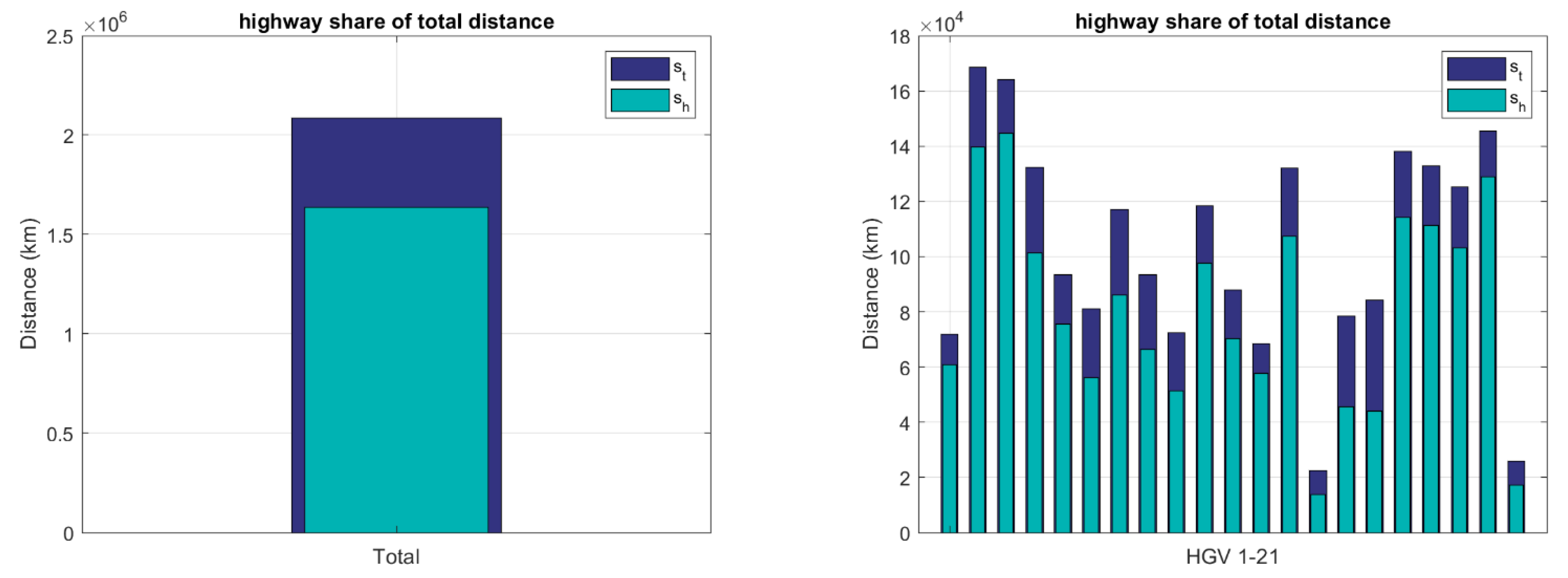
The total distance driven by all the trucks considered in the model is around 2,084,766 km. Of this, 78.45%, or around 1,635,550 km, are on the highway. Looking at the trucks individually, routes with a total distance of 13,860 km to 144,775 km are driven. The highway share is just as wide-ranging. The highway share ranges from a minimum of 52.31% to a maximum of 88.71% (Figure 1).
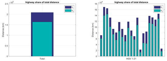
Figure 1.
Share of highways in total distance travelled by all trucks and individually based on ORS evaluation (own illustration).
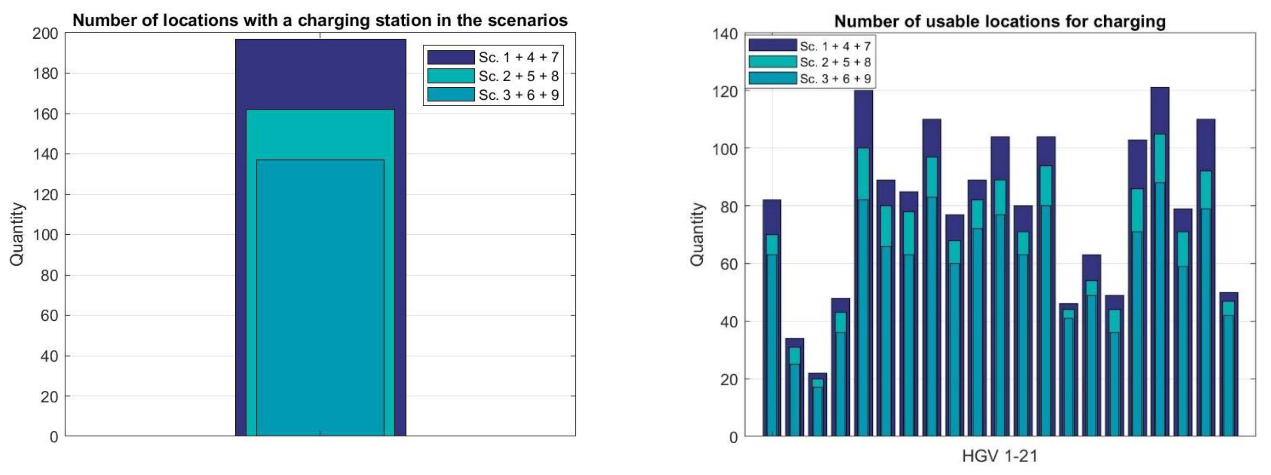
In total, 197 unique locations are accessed by all trucks. In scenarios 1, 4, and 7, at least one charging station is available at all 197 of these locations.
By delineating by average dwell time, the availability of locations with at least a single charging station in Scenarios 2, 5, and 8 is reduced by 17.8% to 162 locations and in Scenarios 3, 6, and 9 by 30.5% to 137 locations that can be used for charging by all trucks. If we look at the actual usable locations of the individual trucks, there is a wide range in the number of locations available for use for the individual trucks. Scenarios 1, 4, and 7 offer a minimum of 22 and a maximum of 121 locations; scenarios 2, 5, and 8 offer a minimum of 20 and a maximum of 105 locations; scenarios 3, 6, and 9 are left with 17 to 88 locations that can be used for loading the accumulator (Figure 2).

Figure 2.
Number of locations with charging station according to scenarios for all trucks and individually (own illustration).
The distance between locations available for the use of charging is around 66 km in the scenarios without restriction, 69 km with 30% restriction, and increases to roughly 71 km in those scenarios with 20% restriction. When looking at the average distance between the charging locations of the individual trucks, the distance varies greatly. For those scenarios without restriction of the charging locations, the distance lies between 14.3 km and 96.9 km; with 30% restriction, it is between 15.3 km and 99.5 km; with 20% restriction, it is between 15.6 km and 102.3 km (Figure 3).
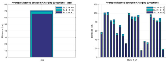
Figure 3.
Average distance between charging locations according to scenarios (own illustration).
For a switch from the diesel trucks considered in the data to purely electrically powered trucks in the model, an average consumption results for each truck separately for highway and non-highway routes. The calculated average consumption on highway routes ranges between 0.9696 kWh/km and 1.4068 kWh/km. On the other hand, the average consumption on nonhighway routes ranges from 1.2666 kWh/km to 1.8311 kWh/km. Overall, an average of 1.5007 kWh/km can be calculated for nonhighway and 1.1366 kWh/km on highway routes. Thus, the consumption on the highway is 24.3% lower than on nonhighway routes (Figure 4).
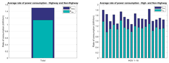
Figure 4.
Average consumption of highway and nonhighway routes (own illustration).
3.2. Required Battery Capacities
The following results are obtained for the minimum required starting energies in the battery in the 9 scenarios considered.
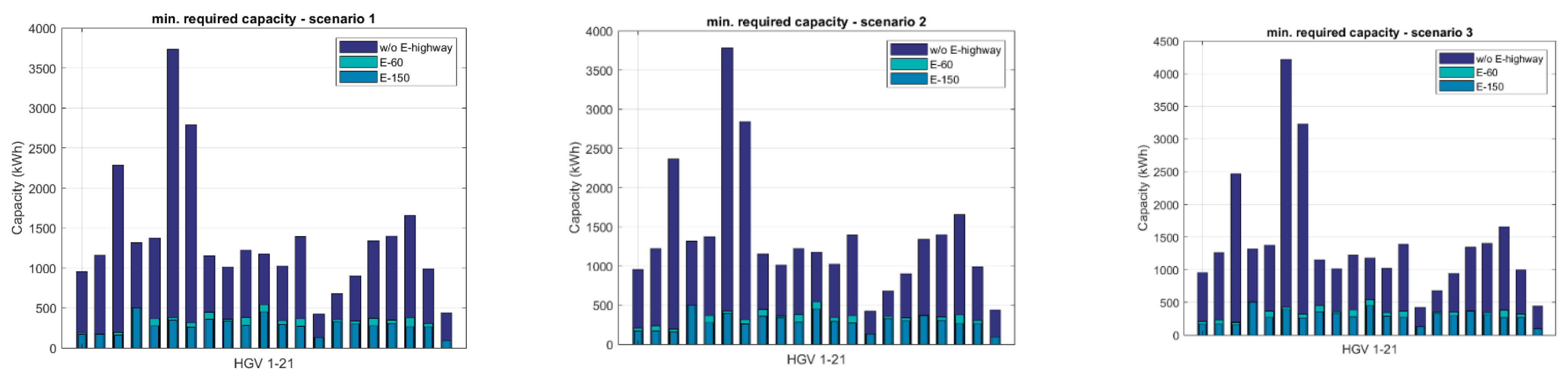
For scenario 1, the minimum capacity required without using an OLS is around 423 kWh to 3734.8 kWh. This compares to minimum required capacities of 92.3 kWh to 541.9 kWh when using OLS with 60 kW (E-60) capacity. An OLS with 150 kW (E-150) allows a reduction to 92.3 kWh to 500.8 kWh. There is only a slight difference to Scenarios 2 and 3, where the required capacities range between 423 kWh and 3783.7 kWh (Sc.2) and 423 kWh and 4224 kWh (Sc. 3) if an OLS is not used, whereas using an OLS reduces the capacities to 92.3 kWh to 541.9 kWh (E-60) and 92.3 kWh to 500.8 kWh (E-150) (Figure 5).
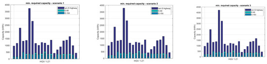
Figure 5.
Minimum required capacity—50 kW charging stations—scenarios 1–3 (own illustration).
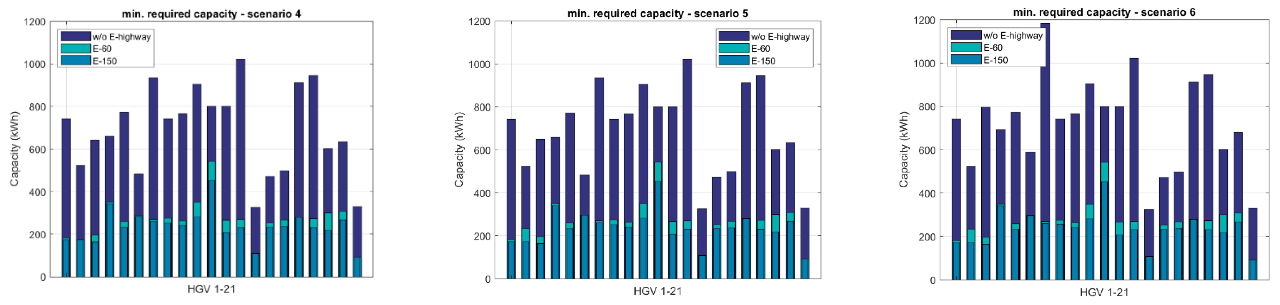
In scenarios 4 to 6, a significant saving in required battery capacity is visible compared to scenarios 1 to 3. This reduction is due to the higher power of the charging stations of 150 kW. In scenario 4, the required battery capacities without using an OLS now range from 324.7 kWh to 1022.6 kWh, while using an OLS, the required capacities are reduced to 92.3 kWh to 541.9 kWh (E-60) and 92.3 kWh to 452.4 kWh (E-150). The required capacities of scenario 5 lie between 324.7 kWh and 1022.6 kWh without OLS, 92.3 kWh and 541.9 kWh (E-60), and 92.3 kWh and 452.4 kWh (E-150). Although the ranges are the same for scenario 4 and 5, there are slight differences looking at the trucks individually. Scenario 6 has an increase in capacities needed, which lie between 324.7 kWh and 1184 kWh (w/o E-highway), 92.3 kWh and 541.9 kWh (E-60), and 92.3 kWh and 452.4 kWh (E-150) (Figure 6).
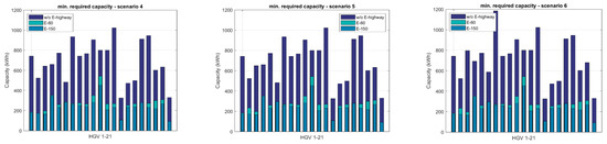
Figure 6.
Required minimum capacity—150 kW charging stations—scenarios 4–6 (own illustration).
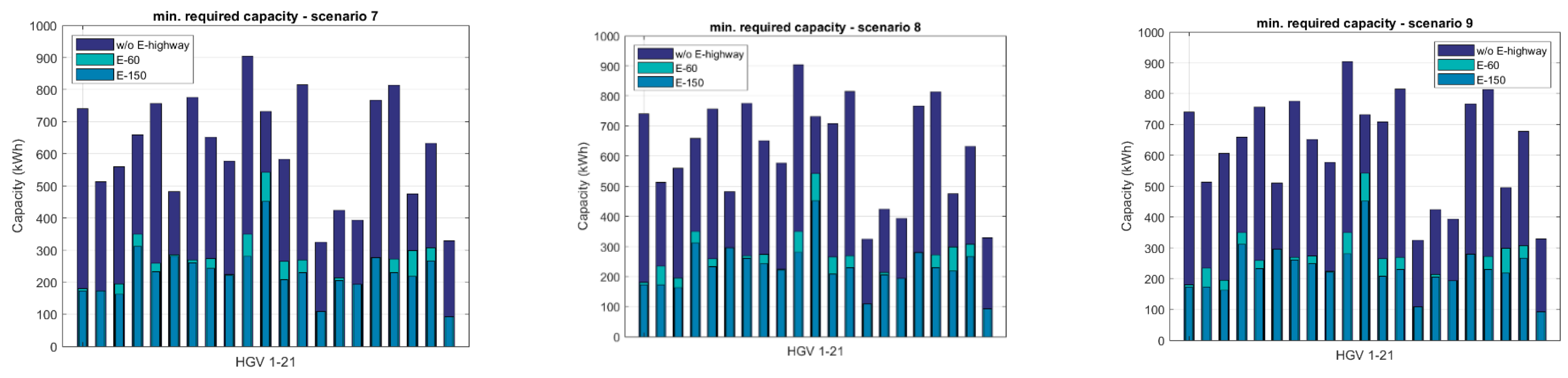
Looking at scenarios 7–9, yet again, there is a decrease in the required capacities visible. In scenario 7, the capacities range from 324.7 kWh to 904.3 kWh (w/o E-highway), 92.3 kWh to 541.9 kWh (E-60), and 92.3 kWh to 452.4 kWh (E-150). Scenarios 8 and 9 deliver the same ranges, while there are some small differences in between the extreme values (Figure 7).
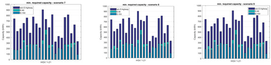
Figure 7.
Minimum required capacity—350 kW charging stations—scenarios 7–9 (own illustration).
The average battery capacity required for all trucks is reduced by 75.9–79.4% from 1355 kWh to 327 kWh (E-60) and 279 kWh (E-150) in Scenario 1 by using OLS. Scenario 2 achieves a 75.6–79.1% reduction from 1366.3 kWh to 333.1 kWh (O-60) and 285.6 kWh (O-150). For Scenario 3, OLS results in a percentage reduction of 76.3–79.8% in minimum species energy from 1414.6 kWh to 334.7 kWh (O-60) and 285.8 kWh (O-150). Scenario 4 achieves an average reduction in battery capacity from 690.8 kWh to 264.5 kWh (O-60) and 235.7 kWh (O-150), or 61.7–65.9%. In Scenario 5, the reduction in battery capacity is from 691.1 kWh to 267.9 kWh (O-60) and 236.5 kWh (O-150), for 61.2–65.8%. For Scenario 6, the average values are 718.7 kWh (without OLS) and 287.9 kWh (O-60) or 236.7 kWh (O-150)—percentage savings of 62.7–67.1%. Scenario 7 results in an average required battery capacity of 614.9 kWh (without OLS), 257.2 kWh (O-60), and 229.7 kWh (O-150) with OLS—resulting in percentage savings of 58.2–62.3%. The capacities calculated for Scenario 8 are 620.9 kWh (without OLS), 260.6 kWh (O-60), or 230.5 kWh (O-150)—this corresponds to a reduction in battery capacity of 58–62.9%. For scenario 9, the values are 627.6 kWh (without OLS) and 260.6 kWh (O-60) or 230.7 kWh (O-150)—the percentage reduction in battery capacity is 58.5–63.2% (Figure 8).
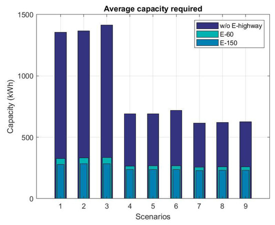
Figure 8.
Minimum required capacity—average of all trucks in each scenario (own illustration).
3.3. Cost Reduction Potential
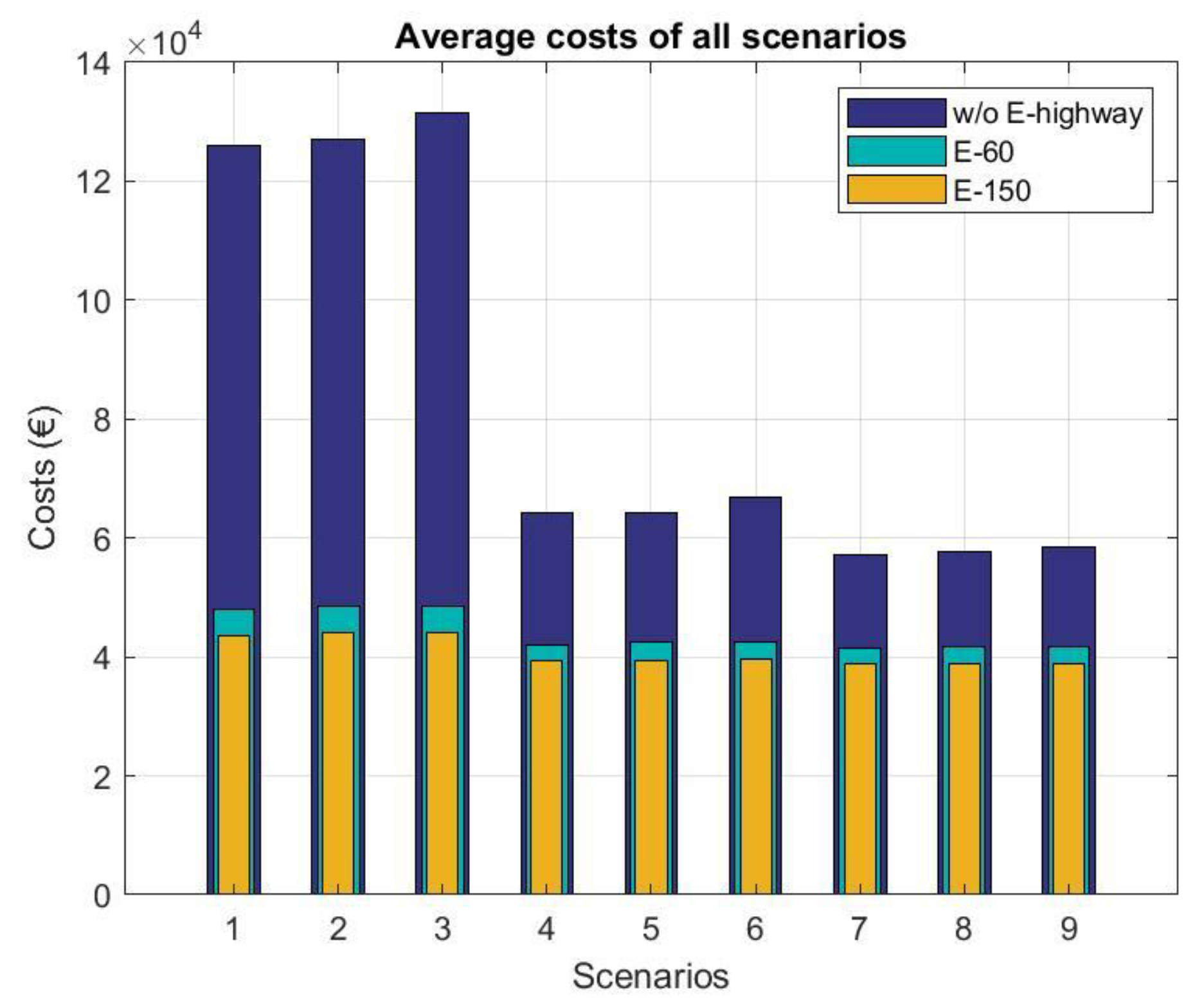
When looking at the average cost reduction of the scenarios, we can see a clear decrease when using an OLS. While the costs without using an E-highway in scenario 1 average around EUR 126,000, they can greatly be reduced by 62–65.5% to an average of EUR 43,456 (E-60) and EUR 38,456 (E-150). In Scenario 2, an average reduction of 61.85–65.33% can be achieved, which reduces the costs from EUR 127,070 to EUR 44,061–48,482. Scenario 3 achieves a reduction of 63–66.49% from EUR 131,550 to EUR 44,082–48,630. In scenario 4, a jump happens, whereas the costs without an OLS are significantly reduced. The average costs of all trucks results in EUR 64,243, which can again be reduced to EUR 39,422–42,095 when operating on an E-highway, which equals a percentage of 34.5–38.6%. In Scenario 5 and 6, the costs without an E-highway slightly increase, while the costs when using one stay mostly the same. Another significant decrease happens in scenarios 7 to 9, where the costs of the accumulator can be reduced by having higher-powered charging stations. The costs here range from EUR 57,187 to 58,363 without using an OLS, which can be reduced to roughly EUR 41,500 (E-60) and EUR 38,900 (E-150). Percentage-wise, the decrease lies between 27.6% and 33.25% (Figure 9).

Figure 9.
Average costs for all trucks of all scenarios (own illustration).
Looking at scenario 8 in detail, not for all trucks, a reduction in costs can be achieved by using a lower-powered OLS of 60 kW. For trucks 6 and 19, the costs of the accumulator and the CCS are slightly higher than the costs of the accumulator without an E-highway. The costs for truck 19 are around 2% higher with an E-highway with 60 kW, but are significantly lower when using an OLS with 150 kW. For truck 6, there is no difference in the costs between the different power levels of the OLS, and they are around 0.06% higher than the costs of operating without an OLS (Figure 10). For these e-trucks, there is little benefit from ERSs due to their routing. The reduction in the battery is lower in cost than the cost of the current collector. This results in a cost disadvantage compared to the benchmark case.
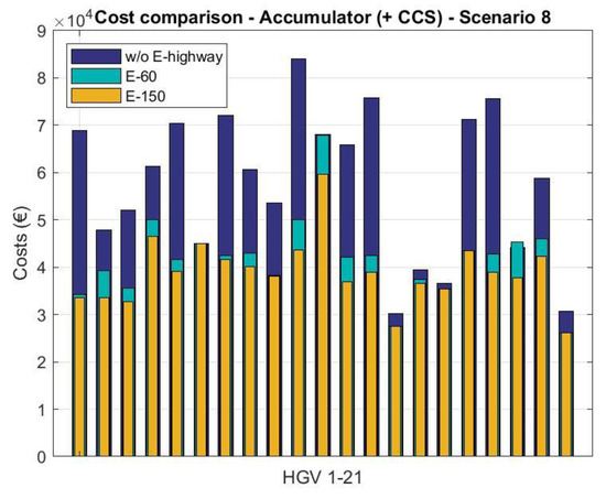
Figure 10.
Costs for trucks individually—350 kW charging stations at 20% of all locations (own illustration).
4. Discussion
The conversion from diesel-powered to purely electrically powered trucks is a challenge for logisticians. On the one hand, they face a financial hurdle due to higher acquisition costs, while on the other hand, charging times and payload restrictions pose a logistical problem. Limited range and longer charging times reduce the flexibility of operating the trucks in long range and two shift operations. It makes it difficult to switch to electric trucks, as it adds new complexity for disposal regarding battery size and SOC.
The aim of this paper was to consider an e-highway as a possible solution for reducing required battery capacities when converting from diesel to electric-powered trucks. For this purpose, a model for calculating the required battery capacities was created using primary data from Schachinger Logistik GmbH. Calculations were performed using ORS and MATLAB to present the effects of an e-highway on required battery capacities. In the model, different scenarios were established, to not only look at the potential reductions in required capacity but also on the loading infrastructure needed.
This paper provides initial insights based on a real-life use case. Due to the chosen methodology, there are certain limitations. First, a very specific use case was selected. Construction logistics is more difficult to equip with stationary charging infrastructure due to the constantly changing destinations. In this case, the whole of Austria is supplied from just one logistics hub. This results in longer driving distances with generally higher highway share. Other logistics cases, such as food logistics, certainly benefit less from the use of ERSs.
The second limitation concerns the determination of electricity consumption. Here, the measured diesel consumption with an average e-truck consumption was used for determination. This only provides a rough estimate, as other consumption levels are to be expected due to the different inherent weights as well as the recuperation of the e-truck. In future work, an existing model will be used to calculate consumption by taking account of differences in altitude, speeds, and loads. Nevertheless, interesting results are obtained for this application.
The results show high reduction potential, keeping the average required capacities in all scenarios below 350 kWh. Having a higher-powered OLS of 150 kW nets slightly better results, but a major effect can still be achieved with a power of 60 kW. Interestingly, there is only a slight increase in capacity needed when decreasing the number of locations with available loading infrastructure. While without the use of an OLS, the distribution of charging stations, as well as their power, play an important role in reducing capacity, this is less significant when an OLS is used. Higher-powered loading infrastructure in combination with wide availability shows a significant decrease when not using an e-highway—the effect is smaller when using an e-highway. This goes to show the potential of an OLS both on the reduction in battery capacity and loading locations needed.
Due to the model-like representation, results regarding concrete consumption on highway and nonhighway routes, as well as battery capacities, must be viewed critically. In the calculations, a constant charging power at the charging stations was assumed, which promises a linear charging of the accumulator. In a real implementation, a nonlinear charging process must be assumed, which must be examined in the specific case. While an attempt has been made to match values as closely as possible to reality, the calculations made are an approximation. Thus, the result of this work primarily aims at presenting the advantages of a potential e-highway for logistics companies operating on Austria’s roads, but can also be considered from the regulatory side when it comes to incentivizing sustainable logistics solutions from the political side.
From the point of view of entrepreneurs, a recommendation can be made for an e-highway when switching to e-trucks, as they do not have to pay for the costs of setting up the e-highway but benefit from considerable savings and advantages. It can be assumed that adjustments to route planning and the truck fleet will have to be made to benefit from an e-highway in the best possible way.
While various pilot projects are underway in countries such as Germany, Sweden, and the USA to implement an e-highway, no projects are currently underway in Austria. With the approach of reducing local GHG emissions in combination with renewable energy yields, an increasing independence of the Austrian energy sector could, thus, be incentivized, which must be implemented on the political side.
What is most important for logistic operators is to route trucks flexibly in Europe. Thus, adaption of significant parts of the TEN-T network is crucial. Economic incentives such as road toll exemptions and free power consumption on e-highways until 2030 will be a significant enhancer of quick adoption of e-highway trucks by logistic operators.
Author Contributions
Conceptualization, T.P.; Formal analysis, T.M.; Funding acquisition, W.M.; Investigation, W.M.; Methodology, T.M.; Supervision, D.W., T.M. and T.P.; Validation, D.W.; Visualization, L.N.; Writing—original draft, L.N.; Writing—review & editing, D.W. All authors have read and agreed to the published version of the manuscript.
Funding
This work was funded in the Programme Line “Austrian Electric Mobility Flagship Projects-9th call”—An initiative of the Federal Ministry for Transport, innovation and Technology (Nr.: 867706). We gratefully acknowledge financial support from the Austrian Ministry for Transport, Innovation and Technology and the Austrian Research Promotion Agency (FFG), the Austrian Climate and Energiefund (KLIEN) and the Kommunalkredit Public Consulting GmbH (KPC).
Institutional Review Board Statement
Not applicable.
Informed Consent Statement
Not applicable.
Data Availability Statement
Additional data can be found at https://megawattlogistics.boku.ac.at/ (accessed on 22 September 2022).
Conflicts of Interest
The authors declare no conflict of interest. The funders had no role in the design of the study; in the collection, analyses, or interpretation of data; in the writing of the manuscript, or in the decision to publish the results.
Nomenclature
| Variable | Description | Unit |
|---|---|---|
| Electric energy consumption per route on highway routes | [kWh/km] | |
| Electric energy consumption per route on nonhighway routes | [kWh/km] | |
| Electric energy consumption per route | [kWh] | |
| Charging power at the charging locations | [kWh] | |
| Charging power on the highway with OLS per route | [kWh] | |
| Remaining energy in the battery | [kWh] | |
| Remaining energy in the battery when using an OLS | [kWh] | |
| Electric energy consumption on a highway section in a route segment | [kWh] | |
| Energy consumption on a nonhighway route in a route segment | [kWh] | |
| Distance of the highway section of the respective route | [km] | |
| Total distance of the respective route | [km] | |
| Average length of stay at the location | [s] | |
| Dwell time on highway section in a route segment | [s] | |
| Average speed between two locations | [km/h] | |
| Diesel consumption | [L] | |
| Maximum depth of discharge | [L] | |
| Loss of charge—vehicle | [L] | |
| Transmission loss—converter | [L] | |
| Loss of charge—charging station | [L] | |
| Loss of energy content due to arrangement to battery set | [%] | |
| Transmission loss—pantograph | [L] | |
| TtW—Diesel vehicle | [%] | |
| TtW—Electric vehicle | [%] | |
| Average energy consumption on highway routes | [kWh/km] | |
| Average electrical energy consumption of all trucks on highway routes | [kWh/km] | |
| Smallest required energy content of the battery | [kWh] | |
| Avg. smallest required energy content of the batteries | [kWh] | |
| Smallest required energy content of the battery when using an OLS | [kWh] | |
| Average smallest required energy content of the battery when using an OLS | [kWh] | |
| Average energy consumption of a truck on nonhighway routes | [kWh/km] | |
| Average electrical energy consumption of all trucks on nonhighway routes | [kWh/km] | |
| Energy content accumulator | [kWh/kg] | |
| Calorific value of diesel | [kWh/L] | |
| Battery cost | [EUR] | |
| Cost of the battery + current collector system when using OLS | [EUR] | |
| Average world market price of battery in 2030 | [EUR/kWh] | |
| Charging power at locations | [kW] | |
| Charging power—overhead line | [kW] | |
| Costs for the current collector system | [EUR] | |
| Distance on the highway | [km] | |
| Total distance travelled | [km] |
Appendix A
First, Docker for Windows is installed. Then, using the Windows command prompt (CMD), a map of ORS to Docker can be installed. To do this, >>docker pull openrouteservice/openrouteservice<< is executed. To be able to make queries about a selected geographic area, the associated OSM file must be downloaded in pbf-format. This can be performed at download.geofabrik.de for the corresponding area. In the context of this work, the file europe-latest.osm.pbf is used for this purpose, which covers the area of Europe. The downloaded file is subsequently packed into a fixed file directory—C:/Temp is suitable for this. In the same directory, a folder named Docker is created. Now, to create the private backend for this area, the following code is executed in the CMD:
docker run -dt –name ors-app -p 8080:8080 -v C:/Temp/Docker/graphs:/ors-core/data/graphs -v D:/Temp/Docker/elevation_cache:/ors-core/data/elevation_cache -v C:/Temp/Docker/conf:/ors-conf -v C:/Temp/dach-latest.osm. pbf:/ors-core/data/osm_file.pbf -e “JAVA_OPTS=-Djava.awt.headless=true -server -XX:TargetSurvivorRatio=75 -XX:SurvivorRatio=64 -XX:MaxTenuringThreshold=3 -XX:+UseG1GC -XX:ParallelGCThreads=8 -Xms1g -Xmx64g” -e “CATALINA_OPTS=-Dcom. Sun.management.jmxremote -Dcom.sun.management.jmxremote.port=9001 -Dcom.sun.management.jmxremote.rmi.port=9001 -Dcom.sun.management.jmxremote.authenticate=false -Dcom.sun.management.jmxremote.ssl=false -Djava.rmi.server.hostname=localhost” openrouteservice/openrouteservice:latest
This code must be adjusted accordingly to the chosen directory and territory. After executing the code, the private ORS backend will be created. This can take several hours depending on the size of the territory and the hardware used. To provide enough RAM, the parameters -Xms1g and -Xmx64g can be adjusted. A higher numerical value provides more RAM. As soon as the creation has been carried out successfully, the address http://localhost:8080/ors/health (accessed on 22 March 2022) can be retrieved and will output {“status”: “ready”}. Adjustments to the restrictions and profiles used (Car, HGV, etc.) can be made in the app.config file, which is automatically created in the selected directory in the Docker folder and subsequently in the config folder. To assert these customizations, the created Docker container must be restarted. Queries via Python can be made after replacing the base URL openrouteservice.org with localhost:8080 or 127.0.0.1:8080 and, thus, using the ORS backend.
Appendix B
To identify the exact duration a truck spends on a way category between two locations, first, those waypoints must be identified, which have the crucial way categories and, consequently, they must be matched with the respective time. ORS outputs both information separately and partly noncongruently. This means that it is not always possible to clearly assign an output time to a waypoint category. Thus, both information must be queried in two different Python scripts, transferred into an Excel file, and finally adapted in MATLAB. The adjustment is carried out in such a way that the time is divided among the way categories based on the proportion of distances between waypoints. The procedure is shown as an example in Figure A1. Line 4 shows a duration of 584.7 s from waypoint 115 to 219. These waypoints are not congruent with those indicating the way category (“WC”).
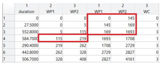
Figure A1.
Problem of unequal coverage of waypoints of way category and duration (own representation).
Figure A1.
Problem of unequal coverage of waypoints of way category and duration (own representation).
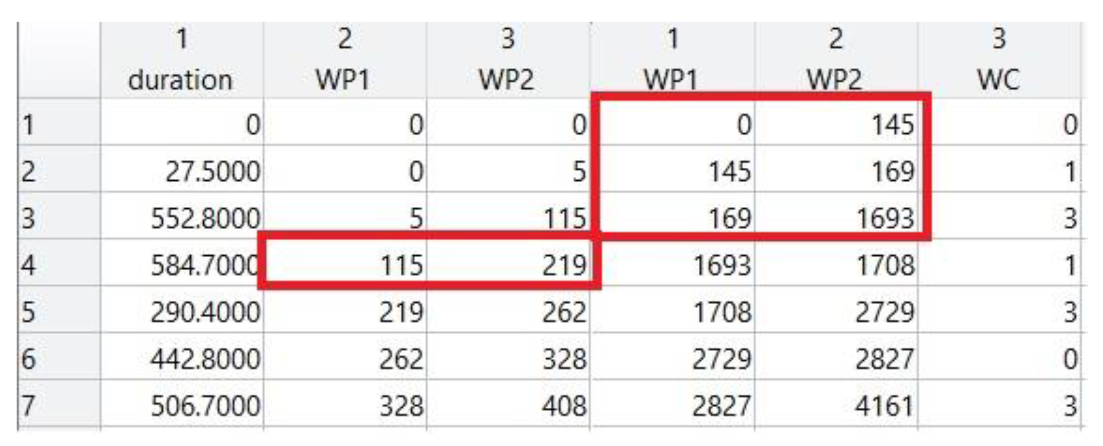
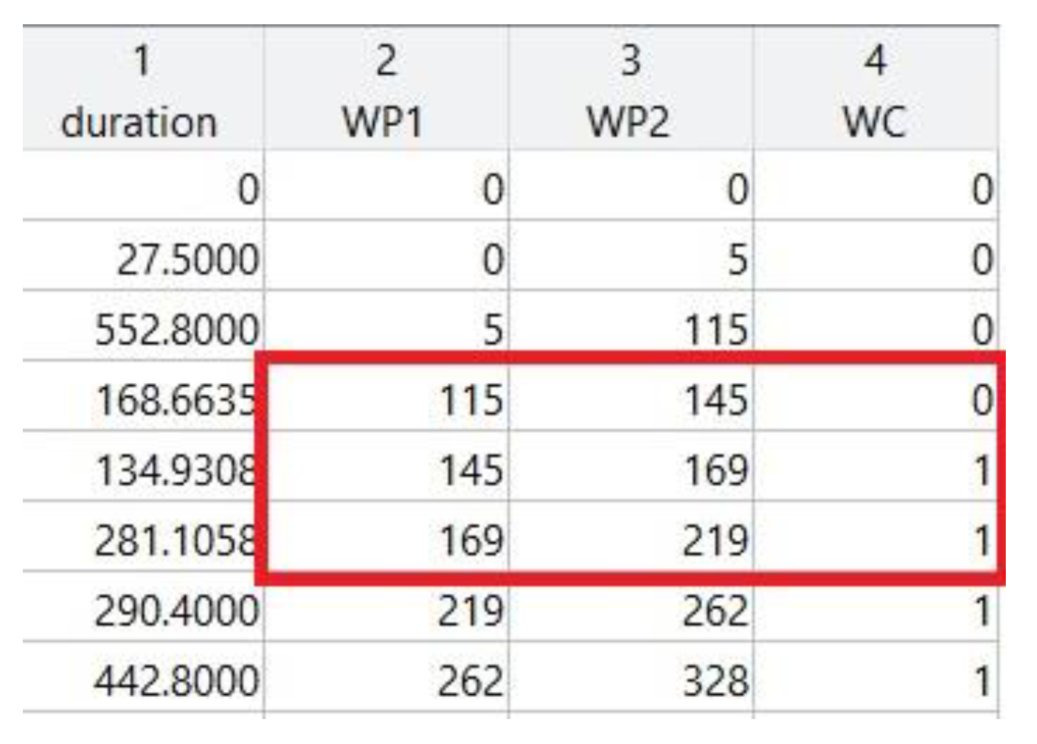
Thus, a delimitation must be made for the specific case so that the duration is divided among the appropriate categories. It is assumed that each distance between two waypoints is of equal length. The duration of 584.7 s, thus, has 104 (219–115) shares. According to the proportions, the duration is divided among the way categories in sequence. Thus, 30 (145–115) shares are in path category 0, 24 (169–145) shares are in path category 1, and 50 (219–169) shares are in path category 3. Line 4 is accordingly divided into 3 new lines and the original line 4 is removed.
The table will look according to the executed code, as shown in Figure A2. It should be noted that in a further step, all path categories indicating a highway (1 and 3) are standardized to a value of 1, as further calculations are subsequently performed using a binary approach.

Figure A2.
Solution of the coverage of path category and duration (own illustration).
Figure A2.
Solution of the coverage of path category and duration (own illustration).
References
- European Commission. A Clean Planet for All. A European Strategic Long-Term Vision for a Prosperous, Modern, Competitive and Climate Neutral Economy. 2018. Available online: https://eur-lex.europa.eu/legal-content/EN/TXT/PDF/?uri=CELEX:52018DC0773&from=DE (accessed on 22 March 2022).
- Anderl, M.; Bartel, A.; Geiger, K.; Gugele, B.; Gössl, M.; Haider, S.; Heinfellner, H.; Heller, C.; Köther, T.; Krutzler, T.; et al. Klimaschutzbericht. 2020. Available online: https://www.umweltbundesamt.at/fileadmin/site/publikationen/rep0776.pdf (accessed on 22 March 2022).
- GmbH, S. Anteil an Treibhausgas-Emissionen in Österreich nach Sektor von 2013 bis 2018. Available online: https://de.statista.com/statistik/daten/studie/961611/umfrage/anteil-an-treibhausgas-emissionen-in-oesterreich-nach-sektor/ (accessed on 22 March 2022).
- Anderl, M.; Friedrich, A.; Gangl, M.; Haider, S.; Köther, T.; Kriech, M.; Lampert, C.; Mandl, N.; Matthews, B.; Pazdernik, K.; et al. Austria‘s National Inventory Report 2020. Umweltbundesamt GmbH. Available online: https://www.umweltbundesamt.at/fileadmin/site/publikationen/rep0724.pdf (accessed on 22 March 2022).
- Heinfellner, H. Sachstandsbericht Mobilität Und Mögliche Zielpfade Zur Erreichung Der Klimaziele 2050 Mit Dem Zwischenziel 2030. 2019. Available online: https://www.umweltbundesamt.at/studien-reports/publikationsdetail?pub_id=2268&cHash=3cc666e5b22063bb3a507fb26ba7afc6 (accessed on 22 March 2022).
- Statistik Austria. Kfz-Neuzulassungen Jänner bis Dezember 2021. 2022. Available online: https://www.statistik.at/wcm/idc/idcplg?IdcService=GET_PDF_FILE&RevisionSelectionMethod=LatestReleased&dDocName=125345 (accessed on 22 March 2022).
- Statistik Austria. Kfz-Neuzulassungen von Elektro-Kfz im 1. Halbjahr 2021. 2021. Available online: https://www.statistik.at/wcm/idc/idcplg?IdcService=GET_PDF_FILE&RevisionSelectionMethod=LatestReleased&dDocName=126389 (accessed on 22 March 2022).
- Kampker, A.; Vallée, D.; Schnettler, A. (Eds.) Elektromobilität: Grundlagen einer Zukunftstechnologie; Springer: Berlin/Heidelberg, Germany, 2018. [Google Scholar] [CrossRef]
- Gustavsson; Martin, G.H.; Hacker, F. Overview of ERS Concepts and Complementary Technologies. 2019. Available online: https://www.oeko.de/fileadmin/oekodoc/ERS-concepts-and-complementary-technologies.pdf (accessed on 22 March 2022).
- Grahn, M.; Azar, C.; Williander, M.; Anderson, J.E.; Mueller, S.A.; Wallington, T.J. Fuel and vehicle technology choices for passenger vehicles in achieving stringent CO2 targets: Connections between transportation and other energy sectors. Environ. Sci. Technol. 2009, 43, 3365–3371. [Google Scholar] [CrossRef]
- Kuramochi, T.; Höhne, N.; Schaeffer, M.; Cantzler, J.; Hare, B.; Deng, Y.; Blok, K. Ten key short-term sectoral benchmarks to limit warming to 1.5 °C. Clim. Policy 2018, 18, 287–305. [Google Scholar] [CrossRef]
- Taljegard, M.; Thorson, L.; Odenberger, M.; Johnsson, F. Large-scale implementation of electric road systems: Associated costs and the impact on CO2 emissions. Int. J. Sustain. Transp. 2020, 14, 606–619. [Google Scholar] [CrossRef]
- Börjesson, M.; Johansson, M.; Kågeson, P. The economics of electric roads. Transp. Part C Emerg. Technol. 2021, 125, 102990. [Google Scholar] [CrossRef]
- Eichlseder, H.; Klell, M. Wasserstoff in der Fahrzeugtechnik; Vieweg + Teubner Verlag: Wiesbaden, Germany, 2012. [Google Scholar] [CrossRef]
- Fiori, C.; Marzano, V. Modelling energy consumption of electric freight vehicles in urban pickup/delivery operations: Analysis and estimation on a real-world dataset. Transp. Res. Part Transp. Environ. Bd. 2018, 65, 658–673. [Google Scholar] [CrossRef]
- Batteries Europe ETIP. Strategic Research Agenda for Batteries 2020; European Commission: Brussels, Belgium, 2020. Available online: https://ec.europa.eu/energy/topics/technology-and-innovation/batteries-europe/news-articles-and-publications/sra_de (accessed on 24 August 2022).
- Röck, M.; Martin, R.; Hausberger, S. JEC Tank-to-Wheels Report v5: Heavy Duty Vehicles; Publications Office of the European Union: Luxemburg, 2020. Available online: https://publications.jrc.ec.europa.eu/repository/handle/JRC117564 (accessed on 24 August 2022).
- Energie-Control Austria. Leitfaden Netzanschluss. 2016. Available online: https://www.e-control.at/documents/1785851/1811582/e-control-leitfaden-netzanschluss-2016.pdf/fd727695-94d7-4a95-bcdf-1695dab0a16e?t=1468230491062 (accessed on 22 February 2022).
- Plötz, P. Infrastruktur Für Elektro-Lkw im Fernverkehr: Hochleistungsschnelllader und Oberleitung im Vergleich—ein Diskussionspapier; Fraunhofer ISI, Öko Institut, ifeu, Karlsruhe: Berlin/Heidelberg, Germany, 2021; Available online: https://www.oeko.de/publikationen/p-details (accessed on 22 February 2022).
- Hjelkrem, O.A.; Arnesen, P.; Bø, T.A.; Sondell, R.S. Estimation of tank-to-wheel efficiency functions based on type approval data. Appl. Energy 2020, 276, 115463. [Google Scholar] [CrossRef]
- BloombergNEF. Battery Pack Prices Fall to an Average of $132/kWh, But Rising Commodity Prices Start to Bite; BloombergNEF: New York, NY, USA, 2021; Available online: https://about.bnef.com/blog/battery-pack-prices-fall-to-an-average-of-132-kwh-but-rising-commodity-prices-start-to-bite/ (accessed on 23 April 2022).
- Wiener Börse, A.G. Wechselkurse EUR: Wiener Börse. Available online: https://www.wienerborse.at/marktdaten/wechselkurse/price-list-currencies/eur/ (accessed on 23 April 2022).
- Kühnel, S.; Hacker, F.; Görz, W. Oberleitungs-Lkw im Kontext Weiterer Antriebs- und Energieversorgungsoptionen für den Straßengüterfernverkehr; Öko-Institut e.V.: Berlin/Heidelberg, Germany, 2018; Available online: https://www.oeko.de/fileadmin/oekodoc/StratON-O-Lkw-Technologievergleich-2018.pdf (accessed on 23 April 2022).


Publisher’s Note: MDPI stays neutral with regard to jurisdictional claims in published maps and institutional affiliations. |
© 2022 by the authors. Licensee MDPI, Basel, Switzerland. This article is an open access article distributed under the terms and conditions of the Creative Commons Attribution (CC BY) license (https://creativecommons.org/licenses/by/4.0/).