Research on the Relationship between Sediment Concentration and Centrifugal Pump Performance Parameters Based on CFD Mixture Model

Abstract

To study the relationship between sediment concentration and the performance parameters of centrifugal pumps, Jiamakou water supply pumping station with total installed capacity of 30,880 kW was selected to analyze characteristics of the centrifugal pump in this paper. Based on a CFD mixture model, the effects of different sediment concentrations on the movement of solid–liquid two-phase flow and the performance parameters of the centrifugal pump were obtained. Then, fitting equations were established between performance parameters (head, flow rate, shaft power, and efficiency) of the centrifugal pump and sediment concentration at three working conditions (0.8 Q = 2 m³/s, Q = 2.5 m³/s, 1.2 Q = 3 m³/s) by the polynomial least-square method. Calculated values of fitting equations were compared with the measured values in centrifugal pump operation. The results show that, as the sediment concentration increases from 0.1% to 1%, the maximum volume fraction of sediment at blade outlet increased from 0.14% to 1.14%, and the maximum volume fraction of sediment at blade outlet increased from 0.7% to 2.29%. The turbulent kinetic energy inside the centrifugal pump increased from 8.74 m²/s² to 10.78 m²/s². The calculated values of fitting equation are in good agreement with the measured values in centrifugal pump operation, and the maximum errors of head, flow rate, and efficiency are 6.48%, 3.54%, and 2.87%, respectively. Therefore, the reliability of the fitting equations is verified. The research method can provide a reference for the calculation of performance parameters for centrifugal pumps in other water supply pumping stations with sediment-laden flow.

1. Introduction

The Loess Plateau, where the Yellow River flows, has characteristics of fine and loose soil. Therefore, it is easy to cause a large amount of soil and water loss, and this has resulted in the Yellow River occupying the first place in the world for having sediment content. Moreover, the particle size of sediment is small, and the sediment particle size tends to continuously decrease as the process progresses [1,2]. The annual average value of sediment concentration is as high as 37.7 kg/m³, and the sediment particle size is 0.05~0.002 mm in the middle reaches of the Yellow River. At present, double-suction is the device most widely used in centrifugal pump operation. Centrifugal pumps are heavily used in pumping irrigation projects in the Yellow River Basin because of their characteristics to pump high flow rate [3]. Double-suction centrifugal pumps are mostly designed and manufactured under the condition of clean water. However, as the Yellow River has high sediment content, the sediment is moved by the action of water in centrifugal pumps, and in turn, the moving sediment affects the flow structure. This situation affects the flow rate, head, and efficiency of centrifugal pumps to varying degrees, and the structure of centrifugal pumps also produces varying degrees of abrasion. This situation does not only affect the flow and head of centrifugal pumps, but also destroys the structure of the centrifugal pumps, thus shortening their life. In addition, the above effects also reduce the efficiency of centrifugal pumps, cause energy waste, and increase economic losses [4,5,6,7]. Such problems occur not only in the Yellow River Basin, but also in other water supply engineering sites with sediment-laden flow. Therefore, it is necessary to study the characteristic parameters of centrifugal pumps under the condition of sediment-laden flow.

With continuous development of Computational Fluid Dynamics (CFD) simulation technology, numerical simulation methods are widely used in the field of pump research. Ding et al. [8] proposed new code to improve the accuracy and speed of CFD simulation calculations. Combined with the physical model of axial flow pumps, this method can quickly predict the flow rate, pressure, and cavitation in pumps. Buratto et al. [9] studied the influence of three fluids with different viscosities on centrifugal pump performance by numerical simulations. Steinmann et al. [10] used numerical simulations to analyze the flow state in scroll pumps, and they predicted the cavitation effects in scroll pumps based on the Rayleigh–Plesset cavitation model. Zhai et al. [11] used the Lumped Parameter (LP) model and the CFD model for the numerical calculation of fluid movement in axial piston pumps based on the cavitation model, the advantages and disadvantages of which two models were analyzed for the prediction of cavitation effects. Thakkar et al. [12] optimized pump heads and efficiency by combining CFD simulation with response surface methodology and the multi-objective optimization algorithm. In recent years, the study of multiphase flow has become a hot topic in simulations. Wan et al. [13] proposed a multigrid finite element analysis method to analyze solid–liquid two-phase flow containing a large number of solid particles in the liquid. Pagalthivarthi et al. [14] used the Spalart–Allmaras (SA) model and the $k-\epsilon$ model to conduct numerical simulation of solid–liquid two-phase flow, and the results showed that the prediction results of the two models were in good agreement. Additionally, the calculation speed of the Spalart–Allmaras (SA) model was relatively fast. In order to calculate the flow parameters of a multiphase flowmeter without separation, Kartashev et al. [15] proposed a dynamic model of multiphase flow, which fully considered monodisperse and polydisperse flows. Zhou et al. [16] used the Euler–Euler model to simulate and analyze the wear effect of sediment-laden flow on blades of different lengths in hydraulic turbines. Pathak et al. [17] used the Algebraic Slip Mixture (ASM) model to study the interaction between the dispersion of solid particles and the flow turbulence in a flow field with obstacles. Under the condition of sediment-laden flow, the results of numerical simulation with clean water cannot reflect the real operations of water pumps. Therefore, combining with the theory of solid–liquid two-phase flow, many experts and researchers have conducted research on the numerical simulation of water pumps under the condition of sediment-laden flow [18,19,20,21]. Noon et al. [22] studied the erosion and wear of centrifugal pumps under solid–liquid two-phase flow using numerical simulations, and they found that temperature had a certain influence on the erosion failure of centrifugal pumps. Pagalthivarthi et al. [23] used a mixed characteristic $k-\epsilon$ model and combined it with the solid–liquid two-phase flow theory to study the solid velocity, solid concentration, and solid stress near the wall in a centrifugal pump. Zhang et al. [24] obtained the fitting relation equation of pump speed and flow over time under solid–liquid two-phase flow with testing. Then, combined with numerical simulation, it was concluded that the shaft power of solid–liquid two-phase flow was higher than that of clean water.

However, among those studies of the influences of sediment-laden flow on the performance parameters of centrifugal pumps, few have taken fitting equations to describe the relationship between performance parameters of centrifugal pumps and sediment concentration. In this paper, fitting equations were established to describe the relationship between performance parameters of the centrifugal pump and sediment concentration with a method of combination of numerical simulation and least-square method, which is also the novelty of this study. The variation of performance parameters with different sediment concentrations can be predicted simply, quickly, and accurately based on the research results, which can provide technical support for economical, energy-saving, and safe operation of water supply pumping stations with different sediment concentrations. Moreover, the research method can provide reference for accurate and rapid calculation of performance parameters of centrifugal pumps in other water supply pumping stations with sediment-laden flow.

The structure of this paper is as follows: In Section 2, engineering cases and related mathematical models are introduced. In Section 3, the numerical simulation results are analyzed, and fitting equations are established between the performance parameters of centrifugal pumps and sediment concentration. In Section 4, the conclusions of this study are presented.

2. Materials and Methods

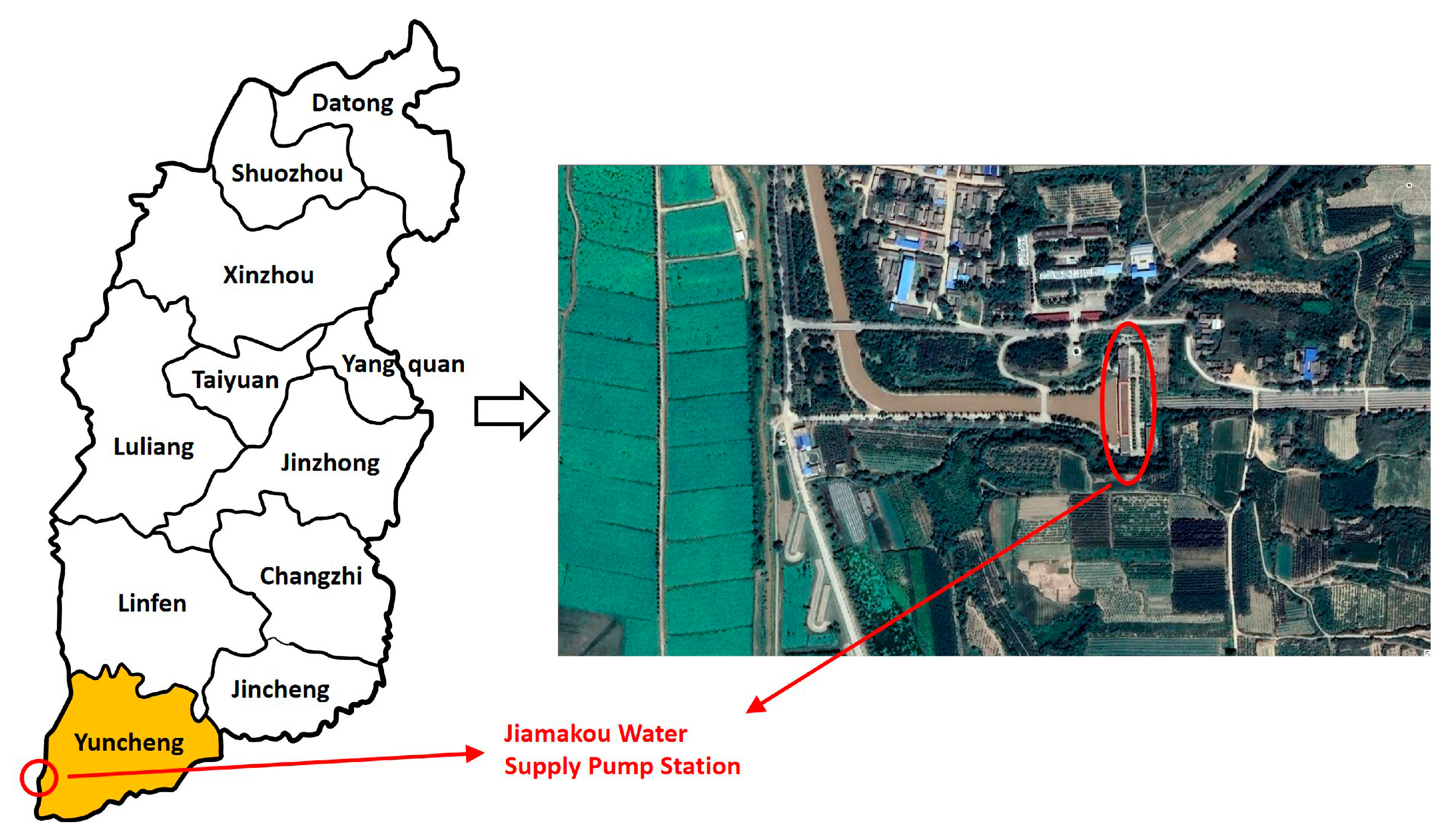
2.1. Research Object

The Jiamakou water supply pumping station is located in Shanxi Province, China [25], as shown in Figure 1. The pumping station has 12 units with total design flow rate of 30.5 m³/s, and total installed capacity of 30,880 kW. The 800S-76 centrifugal pump of the pumping station was selected to explore the performance parameters of the centrifugal pump under different sediment concentrations. The centrifugal pump is a double-suction centrifugal pump with a design flow rate of 2.5 m³/s, and rotational speed of 750 r/min. The impeller has eight groups of blades. The working parameters of the centrifugal pump at 0.8 Q, Q, and 1.2 Q working conditions are shown in

Table 1. Double-suction 800S-76 model centrifugal pump working parameters.

Working Conditions	Head (m)	Flow Rate (m3/s)	Shaft Power (kW)	Efficiency (%)
0.8 Q	79	2	1886.82	82
Q	75	2.5	2160.08	85
1.2 Q	64	3	2292.84	82

. Based on the measured data, the weight sediment concentration of the water flowing through the pump is less than 0.5%, for there is a sedimentation tank in front of the pumping station.

2.2. Mixture Model

The mixture model has the advantage that discrete phases are widely distributed in the computational domain. The mixture model assumes local equilibrium in a short space scale, which can be used to simulate multiphase flow with different velocities of each phase, and the phases have strong coupling. Besides mixture model, there are the VOF (Volume of Fluid) model and Euler model for multiphase flow calculation. However, the VOF model is suitable for stratified flow or free surface flow, and the Euler model is more suitable for discrete phase concentrated in only a part. Therefore, the Mixture model is chosen to calculate the solid–liquid two-phase flow at centrifugal pumps in this paper.

Based on a CFD mixture model [26,27], the solid–liquid two-phase flow of 800S-76 centrifugal pump is simulated numerically. The mixture model uses an algebraic slip equation.

The continuum equation of the mixture model is

$$\frac{\partial }{\partial t}\left({\rho }_m\right)+\nabla ·\left({\rho }_m{v}_m\right)=0$$

(1)

The momentum equation of the mixture model is

$$\frac{\partial }{\partial t}\left({\rho }_m{v}_m\right)+\nabla ·\left({\rho }_m{v}_m{v}_m\right)=-\nabla p+\nabla ·\left[{\mu }_m\left(\nabla v_m+\nabla v_m^T\right)\right]+{\rho }_m+F+\nabla ·\left({\displaystyle \sum }_{k=1}^n{\alpha }_k{\rho }_k{v}_{dr,k}{v}_{dr,k}\right)$$

(2)

where ${\rho }_m$ is mixture density, kg/m³; $v_m$ is mass average velocity, m/s; ${\mu }_m$ is mixture viscous coefficient, Pa·s; $F$ is body force, Pa; $n$ is number of phases (there are only water phase and sediment phase, so $n=2$); ${\alpha }_k$ is volume fraction of the kth phase; ${\rho }_k$ is density of the kth phase, kg/m³; and $v_{dr,k}$ is drift velocity of the kth phase, m/s.

Slip velocity $v_{qp}$ is expressed as the velocity of second phase p (sediment phase) relative to primary phase q (water phase):

$$v_{qp}=v_p-v_q={\tau }_{q,p}a$$

(3)

where ${\tau }_{q,p}$ is relaxation time of particles, s; a is acceleration of second-phase particle (sediment phase), m/s².

In Equation (3), the relaxation time of the particle ${\tau }_{q,p}$ and the acceleration of the second-phase particle are expressed as

$${\tau }_{q,p}=\frac{\left({\rho }_m-{\rho }_p\right)d_p^2}{18{\mu }_q{f}_{dra\mathrm{g}}}$$

(4)

$$a=\mathrm{g}-\left(v_m·\nabla \right)v_m-\frac{\partial v_m}{\partial t}$$

(5)

where ${\rho }_p$ is density of the second phase p, kg/m³; $d_p$ is particle diameter of the second phase p, m; and ${\mu }_q$ is relative dynamic viscosity coefficient of the second phase p, Pa·s.

Resistance equation $f_{drag}$ is expressed as

$$f_{drag}=\{\begin{array}{c}1+0.15R{e}^{0.687} \left(Re\le 1000\right)\\ 0.0183Re \left(Re>1000\right)\end{array}$$

(6)

Finally, the slip velocity $v_{qp}$ is

$$v_{qp}=\frac{\left({\rho }_p-{\rho }_m\right)d_p^2}{18{\mu }_q{f}_{drag}}\left[g-\left(v_m·\nabla \right)v_m-\frac{\partial v_m}{\partial t}\right]$$

(7)

The relationship between drift velocity $v_{dr,p}$ and slip velocity $v_{qp}$ of the second phase p is

$$v_{dr,p}=v_{qp}-{\displaystyle \sum }_{k=1}^n\frac{{\alpha }_k{\rho }_k}{{\rho }_m}{v}_{qk}$$

(8)

The volume fraction equation of second phase p can be obtained from the continuous equation of second phase p, which is expressed as

$$\frac{\partial }{\partial t}\left({\alpha }_p{\rho }_p\right)+\nabla ·\left({\alpha }_p{\rho }_p{v}_m\right)=-\nabla ·\left({\alpha }_p{\rho }_p{v}_{dr,p}\right)$$

(9)

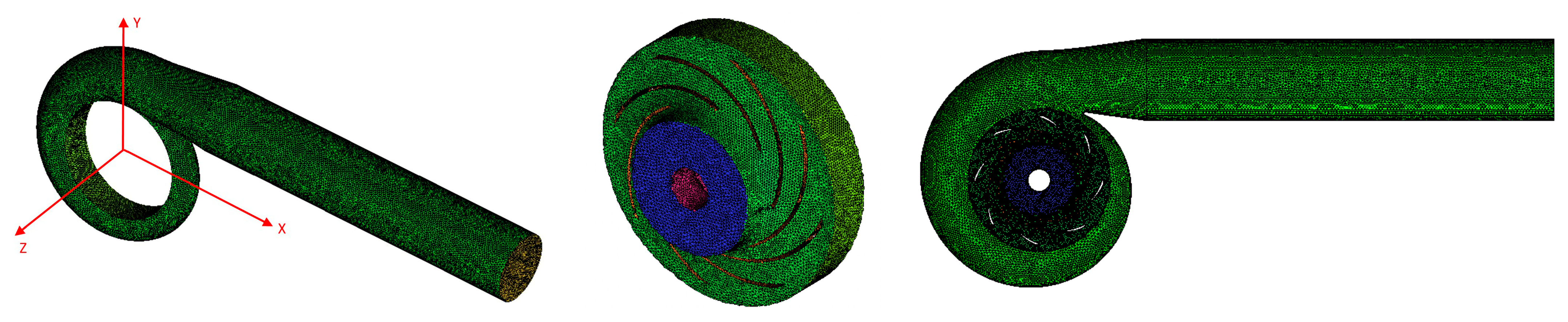
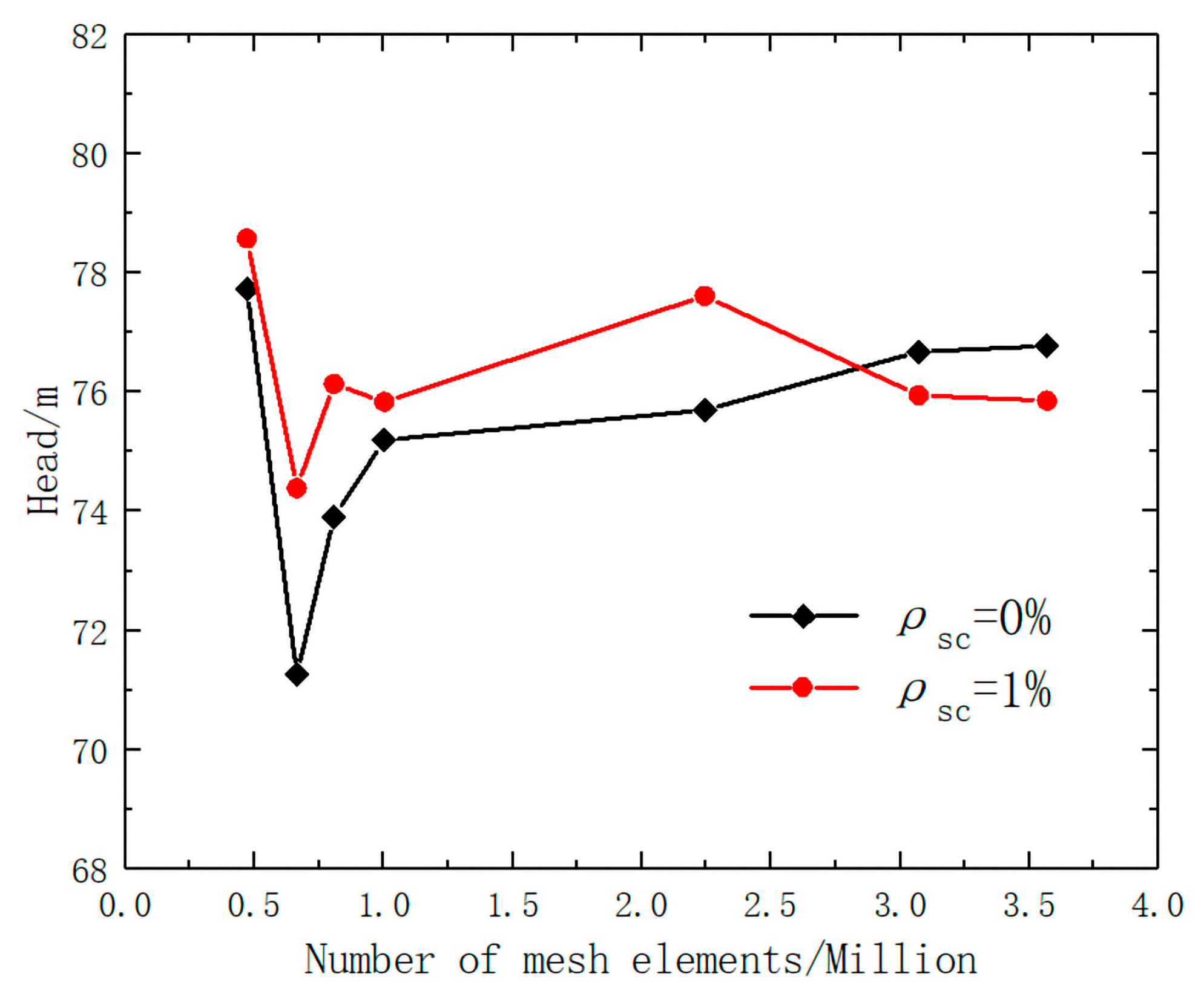
2.3. Meshing and Calculation Method

In this paper, the central point of impeller inlet is taken as the origin of coordinates to establish the coordinate system, as shown in Figure 2. Because the structure of 800S-76 double-suction centrifugal pump is complex, the model of volute and impeller were meshed with an unstructured tetrahedral grid. The model of fluid domain and the grid division are shown in Figure 2. After grid independence analysis, the number of grid elements of volute and impeller are 1,705,886 and 1,365,631, respectively, and the global maximum element seed size of volute and impeller are 24 mm and 14 mm, respectively. The total number of grid elements are 3,071,517. The change curve of the pump head with grid number is shown in Figure 3.

In ANSYS FLUENT 19.0 software [6,24], the inlet boundary condition was speed inlet; the boundary condition of free outflow was selected at the outlet; the condition of no-slip was set for the boundary condition at the wall, and the standard wall function was used for the near wall; the y+ of volute and impeller are about within 3600 and 3000 [28,29]; the static region of the volute and the dynamic region of impeller were coupled by using the MRF model; the $k-\epsilon$ model was selected for the turbulence model; and the solver selected was the SIMPLEC solver.

2.4. Polynomial Least-Squares Fitting Principle

In this paper, the fitting equations are established between the performance parameters of the centrifugal pump and sediment concentration by the polynomial least-squares method, and the characteristic curves of the centrifugal pump are fitted and drawn under different sediment concentrations. The principle of polynomial least-squares fitting is as follows:

Given m + 1 data points $\left(x_i,y_i\right)\left(i=0,1,2,\cdots ,m\right)$, an approximate polynomial function f(x) of order n can be introduced for fitting. That is,

$$f\left(x\right)=a_0+a_{1}x+a_2{x}^2+\cdots +a_n{x}^n={\displaystyle \sum }_{k=0}^n{a}_k{x}^k n<m$$

(10)

In order to satisfy the requirement that an approximate polynomial function can better reflect the trend of data points, the sum of squares of deviation should be minimized between the fitting values of discrete points and data points. That is,

$$\delta ={\displaystyle \sum }_{i=1}^m{\left[f\left(x_i\right)-y_i\right]}^2=min$$

(11)

The above method is the principle of polynomial least-squares method [30,31]. According to this principle, the process of determining a polynomial is essentially the process of determining the coefficient a_k in the polynomial function f(x). Thus, the minimum sum of squares of deviation should be a function of coefficient $a_k\left(0\le k\le n\right)$. That is,

$$S\left(a_0,a_1,a_2,\cdots ,a_n\right)={\displaystyle \sum }_{i=1}^m{\left[f\left(x_i\right)-y_i\right]}^2=min$$

(12)

The solution for the minimum sum of squares of deviations is equal to the extreme value of Equation (16). Thus, the partial derivative of $S\left(a_0,a_1,a_2,\cdots ,a_n\right)$ with respect to $a_k\left(0\le k\le n\right)$ is equal to 0. Each coefficient $a_k\left(0\le k\le n\right)$ in the polynomial can be solved by solving the partial derivative equations. Finally, the fitting polynomial equation is obtained.

Let the straight-line fitting equation be y = a + bx. Class A uncertainty $U_{a,A}$, $U_{a,B}$ is

$$U_{a,A}=t_{0.95}\left(\nu \right)·s_a$$

(13)

$$U_{a,A}=t_{0.95}\left(\nu \right)·s_a$$

(14)

where $t_{0.95}\left(\nu \right)$ is t distribution factor.

The standard deviations of intercept a and slope b are s_a and s_b. That is,

$$s_a=s_y\sqrt{\frac{{\overline{x}}^2}{{\displaystyle \sum }{\left(x_i-\overline{x}\right)}^2}+\frac{1}{n}}$$

(15)

$$s_b=\frac{s_y}{\sqrt{{\displaystyle \sum }{\left(x_i-\overline{x}\right)}^2}}$$

(16)

The standard deviation of dependent variable is

$$s_y=\sqrt{\frac{{\displaystyle \sum }{\left[y_i-\left(a+b{x}_i\right)\right]}^2}{n-2}}$$

(17)

Finally, the uncertainty results of intercept a and slope b are expressed as $A=a_0\pm U_{a,A}$ and $B=b_0\pm U_{b,A}$ ($a_0$ and $b_0$ are specific solutions).

3. Results and Discussion

3.1. Model Validation

When the operation of the centrifugal pump is under the condition of clean water, the head and shaft power of the centrifugal pump are calculated by numerical simulation under the conditions of 0.8 Q, Q, and 1.2 Q. The simulation data are compared with the working parameters of the centrifugal pump, and the results are shown in

Table 2. Errors between simulated values and working parameters.

Working Condition	Head (m)			Shaft Power (kW)
	Working Parameter	Simulated Value	Relative Error	Working Parameters	Simulated Value	Relative Error
0.8 Q	79	79.64	0.81%	1886.82	1921.66	1.85%
Q	75	76.68	2.25%	2160.08	2230.52	3.26%
1.2 Q	64	65.26	1.97%	2292.84	2358.43	2.86%

. The results show that the simulated data are in good agreement with the working parameters of the centrifugal pump, and the maximum error of head and shaft power are only 2.25% and 3.26%.

In actual operation, the centrifugal pump wear is caused by long-term collision between sediment particles and pump components. The larger the volume fraction of sediment particles, the more serious the wear. The volume fraction of sediment particles with the sediment concentration of 1% is predicted by numerical simulation, and the results are shown in Figure 4. The results in Figure 4 show that the predicted results of the volume fraction of sediment particles are consistent with the wear of the impeller in the water supply pumping station. The above results show that the numerical simulation method adopted in this study is reliable.

3.2. Analysis of Simulated Results of Internal and External Characteristics of Centrifugal Pump with Sediment-Laden Flow

The median particle size (d = 0.198 mm) of sediment (density of 2650 kg/m³) in the front pool of the pumping station was selected based on the actual operation of Jiamakou water supply pumping station. The performance of the centrifugal pump at the design flow is studied under the conditions of clean water (the sediment concentration of 0%) and different sediment concentrations, and the effects of those sediment concentrations on internal characteristics and performance parameters of the centrifugal pump, are analyzed.

3.2.1. Internal Characteristic Analysis

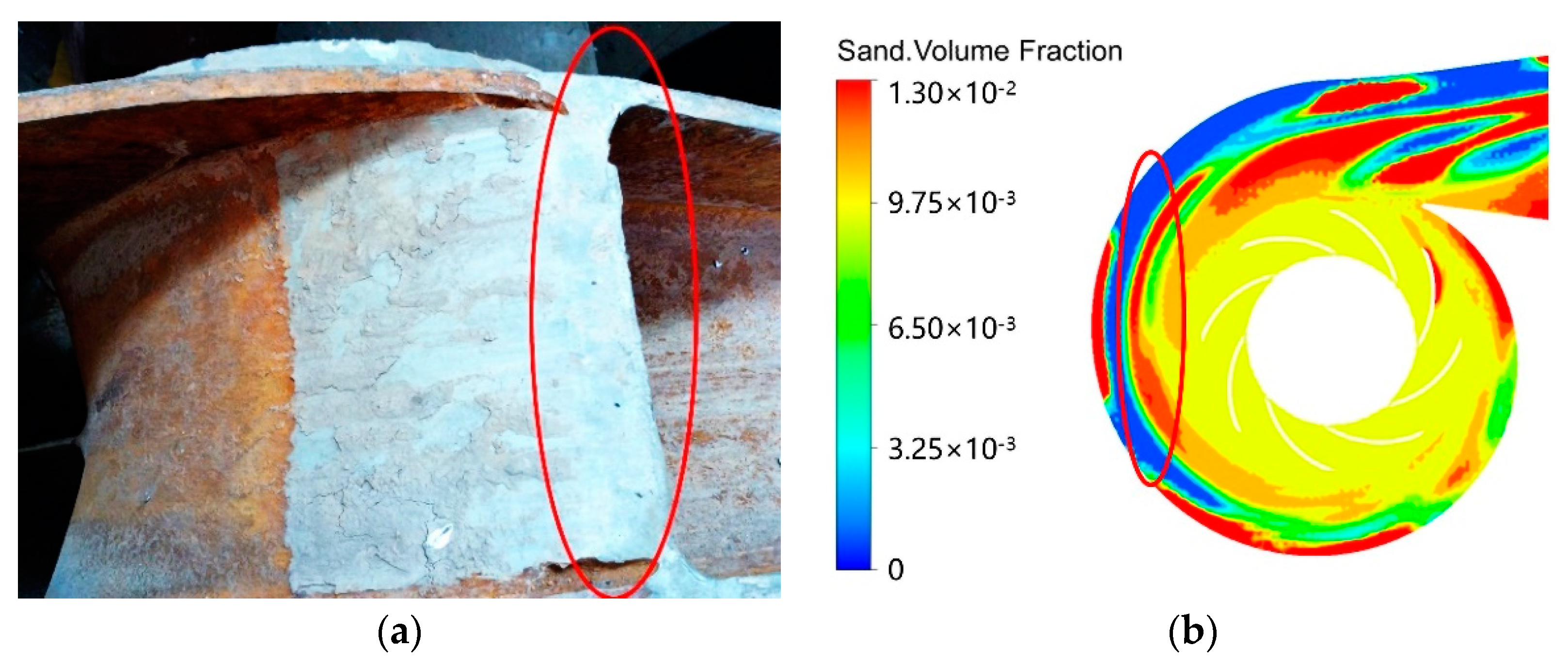
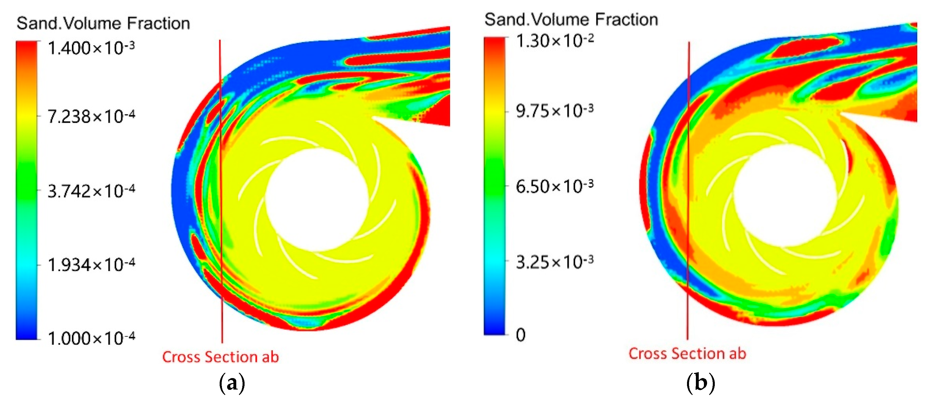
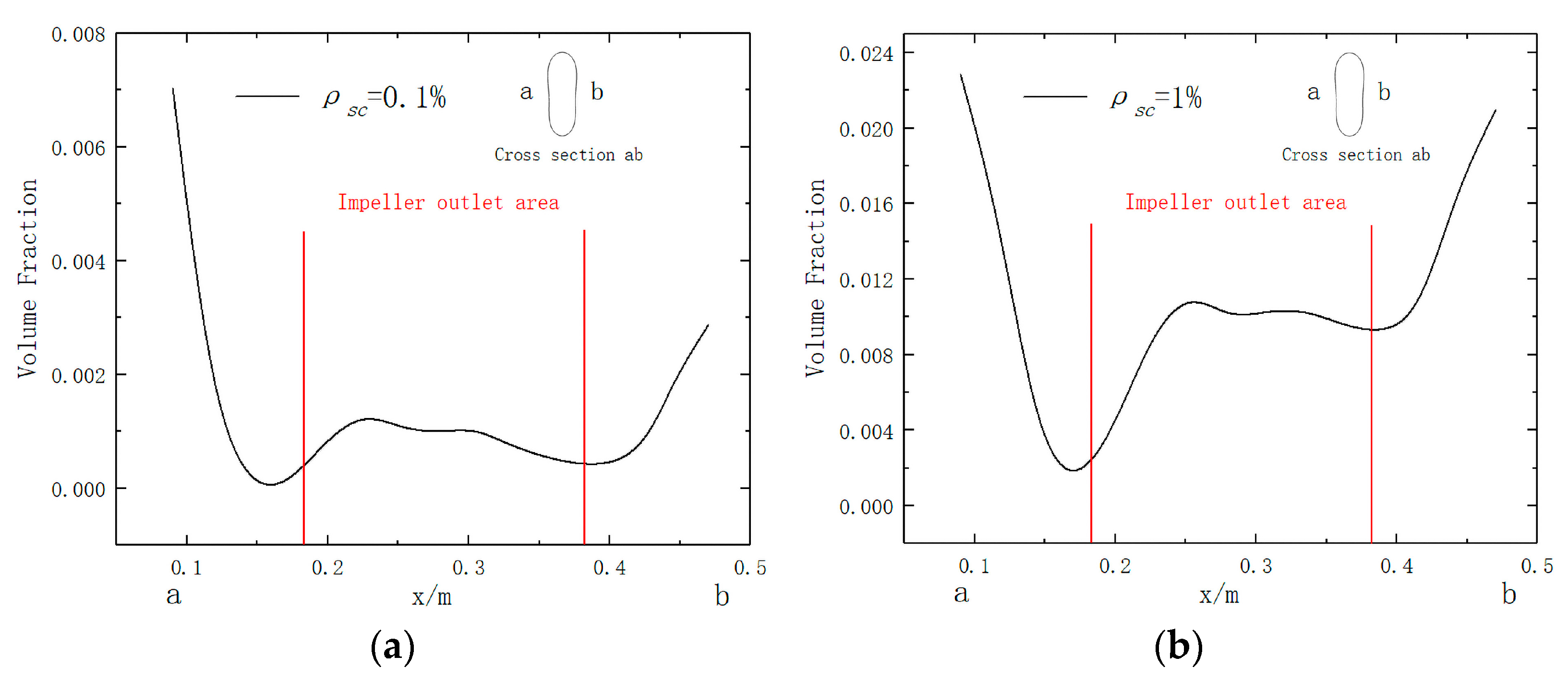
• Influence of sediment concentrations on solid particle distribution in the centrifugal pump

The volume fraction of solid particles in the centrifugal pump under the sediment concentration of 0.1% and 1% are calculated, and the results are shown in Figure 5.

As can be seen in Figure 5, the volume fraction distribution of solid particles at impeller inlet is relatively uniform. The solid particles are affected by the centrifugal force and the inertia force of the impeller, with the result that the solid particles flow into the volute very close to the working surface of the blade. Additionally, some solid particles even collide with blade working surface, resulting in blade surface wear. At the junction between blade outlet and volute inlet, the volume fraction of solid particles is distributed unevenly. The volume fraction of solid particles at blade outlet is relatively high, leading to a greater wear at blade edge and even blade damage. The volume fraction of solid particles is not distributed evenly in volute, and the volume fraction of solid particles in volute wall is higher than that in volute, resulting in a greater volute wall wear.

In Figure 5, the cross-section ab (X = −0.62 m) is selected to analyze the influence of sediment concentrations on the variation of solid particles volume fraction at the impeller outlet in the centrifugal pump, and the results are shown in Figure 6.

According to Figure 5 and Figure 6, the variation law of solid particle volume fraction is similar in the centrifugal pump at sediment concentrations of 0.1% and 1%. The volume fraction of solid particles shows a higher trend at blade edge and volute wall. However, when the sediment concentration increases from 0.1% to 1%, the volume fraction of solid particles increases at the outlet edge of blade and volute wall. The maximum volume fraction of solid particles increases from 0.14% to 1.14% at blade outlet, while the maximum volume fraction of solid particles increases from 0.7% to 2.29% at volute wall. Therefore, the wear degree of blade edge and volute wall also increases.

(2)

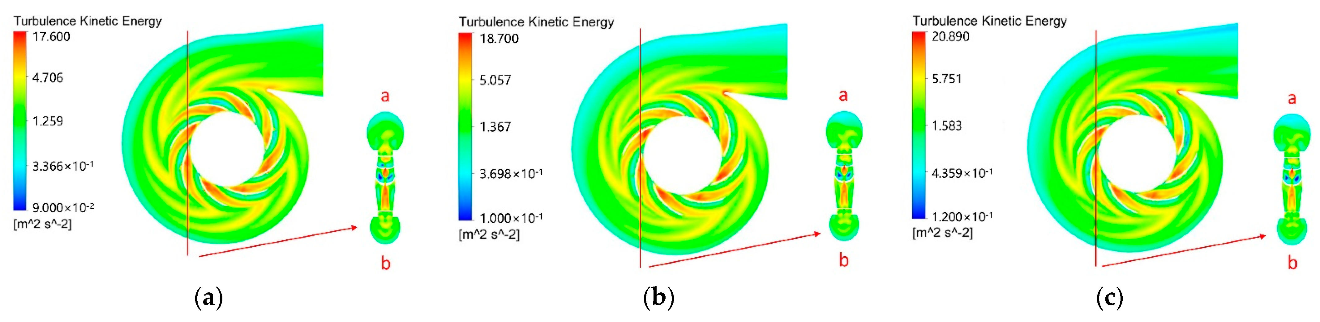
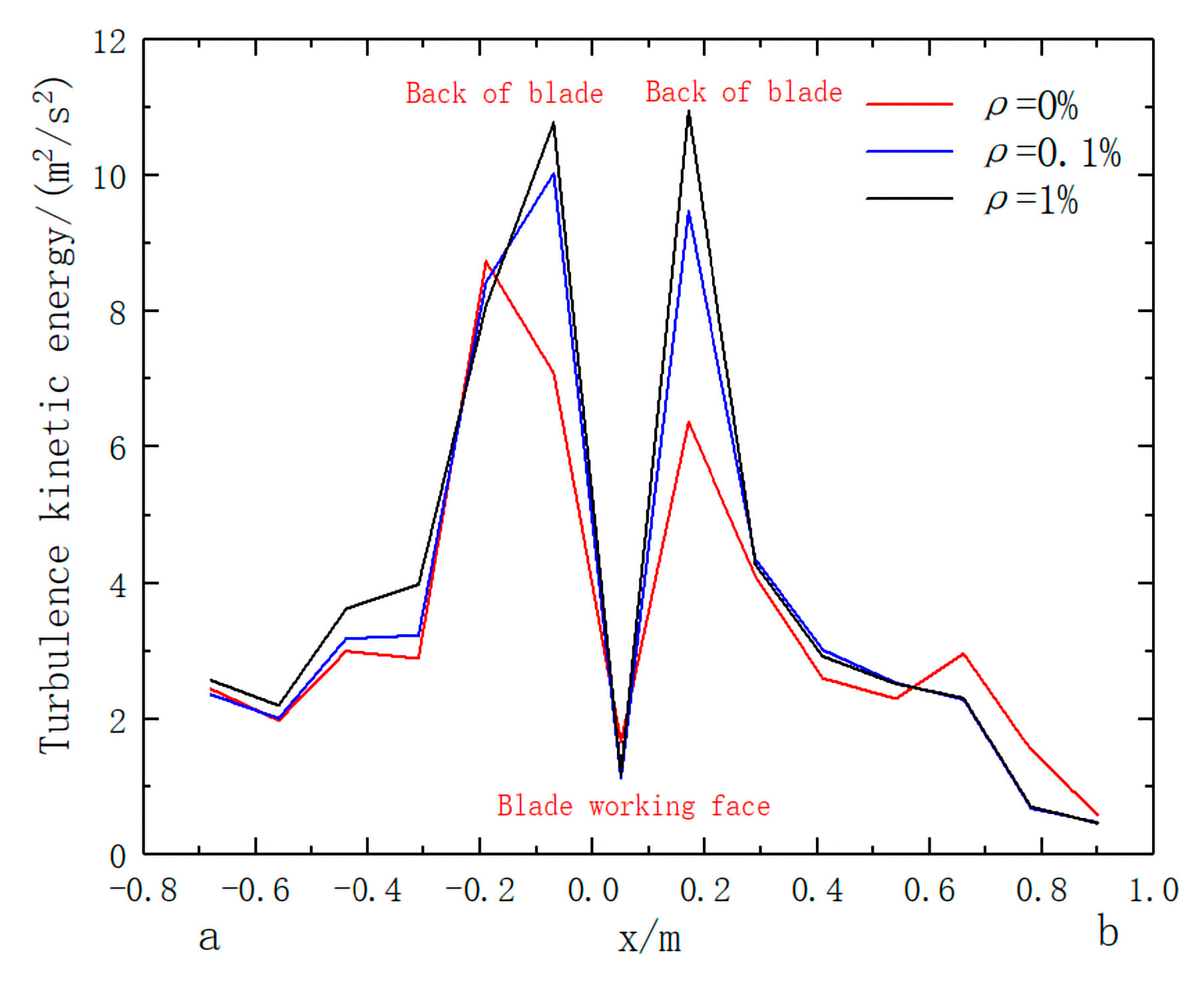
Effect of sediment concentrations on the turbulent kinetic energy in centrifugal pump

The higher the turbulence kinetic energy, the stronger the turbulence vortex in the fluid, and the more energy is consumed by multiphase flow, resulting in increased loss of pressure and energy in the operation of centrifugal pumps [5,32]. The distributions of turbulent kinetic energy in the centrifugal pump under different sediment volume fractions are shown in Figure 7.

As can be seen in Figure 7, the speed and direction of water flow change greatly when clean water flows through the high-speed rotating impeller from the pump inlet, which leads to the increase of turbulence kinetic energy at the impeller inlet. With the deepening of flow, the flow is affected by the superposed effect of axial vortex in impeller, with the result that the relative velocity increases gradually from blade working surface to the back of blade, thus leading to a large turbulent kinetic energy region on the back of blade. At the blade outlet, the velocity and direction of water flow change greatly as the water flows from high-speed rotating impeller into the static volute. Therefore, a relatively large turbulent kinetic energy region appears in impeller outlet and volute inlet. Due to the limitation of centrifugal pump structure, the impact of water flow increases at cochlea tongue. The anisotropic character and the shear stress of the water will change when the water flows into volute through volute tongue, which results in the high turbulent kinetic energy region near the volute tongue.

In Figure 7, the cross-section ab (X = −0.35 m) is selected to analyze the influence of sediment concentrations on the variation of turbulent kinetic energy in the centrifugal pump, and the results are shown in Figure 8.

Figure 7 and Figure 8 show that the turbulent kinetic energy is higher in the centrifugal pump under the condition of sediment-laden flow than that of clean water. Because the density of solid particles is higher than that of water, the motion speed and the trajectory of solid particles are not synchronized with the water after the addition of solid particles. Therefore, wake vortices are produced due to velocity slip in solid–liquid and solid–solid phases, which cause turbulence enhancement. Additionally, more wake vortices are generated due to the velocity slip in solid–liquid and solid-solid phases as the sediment concentration increases from 0% to 1%, which causes the turbulent kinetic energy to increase in the centrifugal pump continuously, and the maximum turbulent kinetic energy increases from 8.74 m²/s² to 10.78 m²/s². Finally, loss of pressure and energy also increase continuously in the process of centrifugal pump operation.

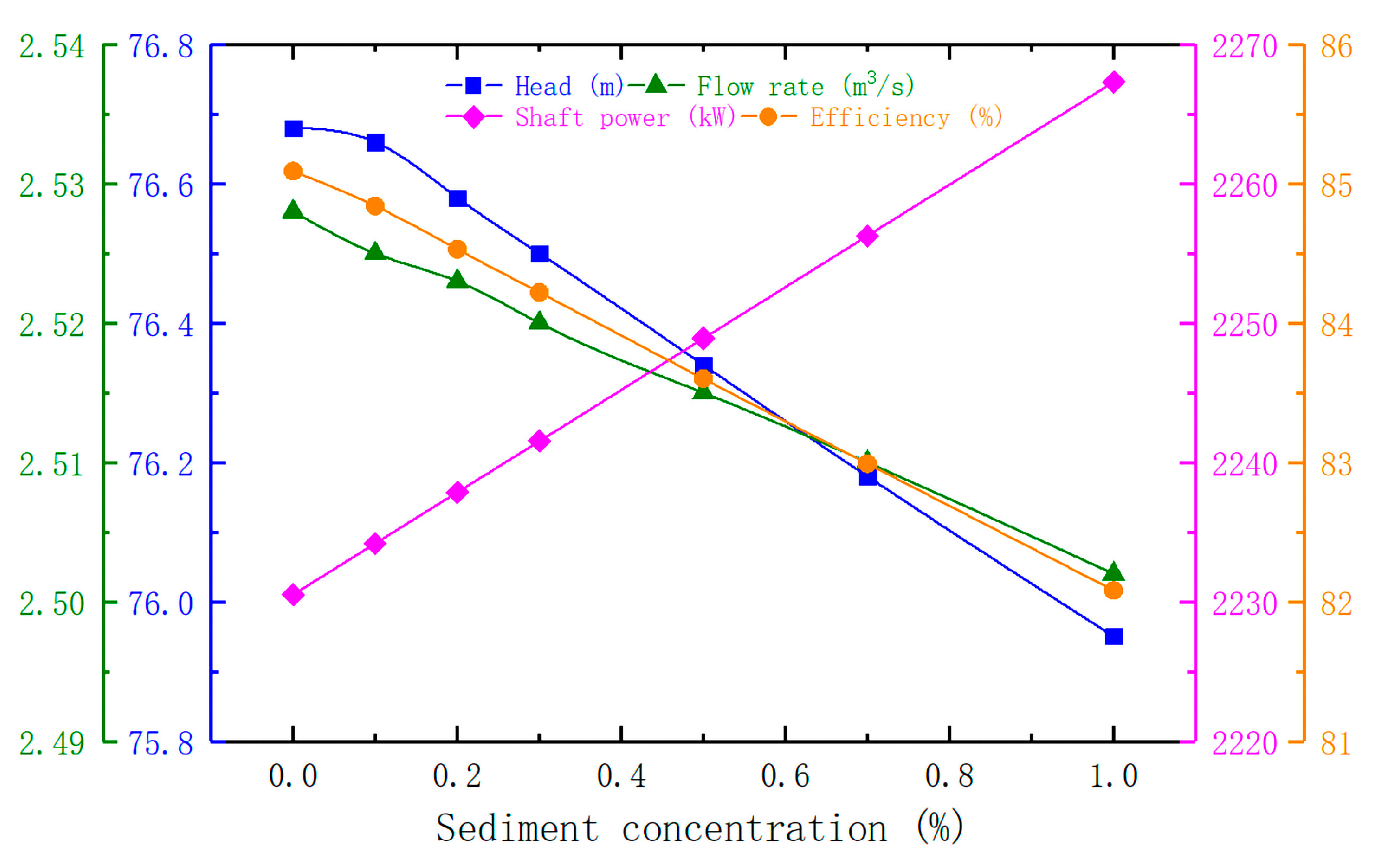
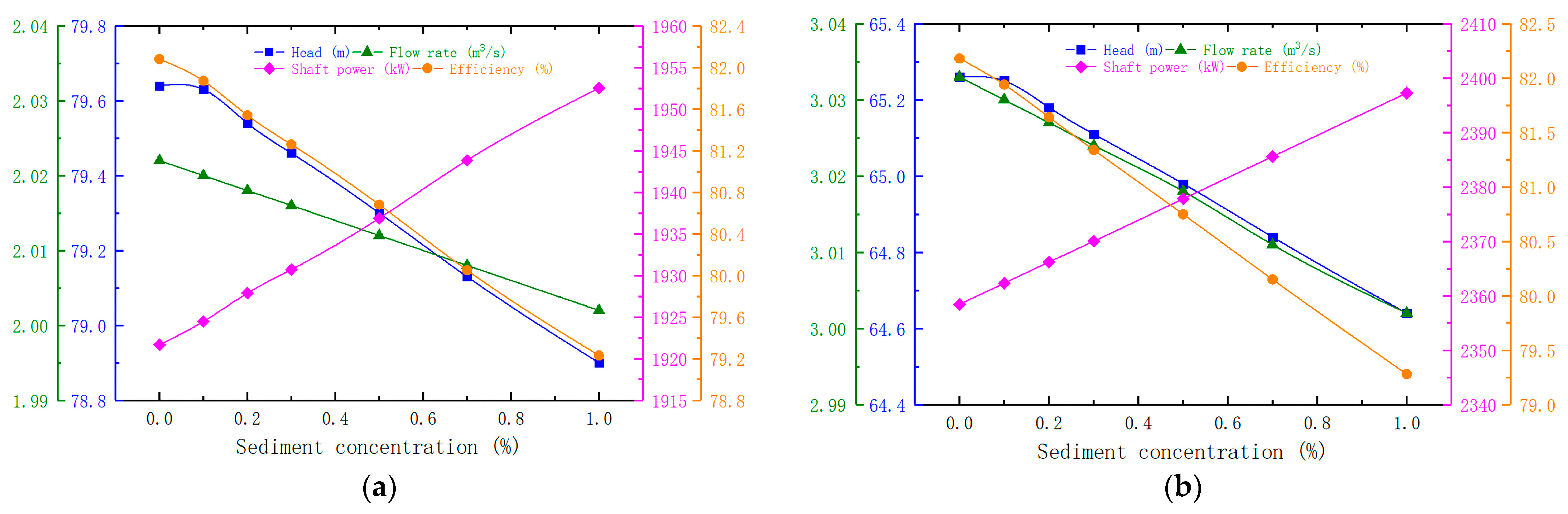
3.2.2. External Characteristic Analysis

The variation laws of head, flow rate, shaft power, and efficiency over different sediment concentrations at the design flow rate Q are obtained by numerical simulation, as shown in

Table 3. Performance parameters of centrifugal pump with different sediment concentrations at design flow rate Q.

ρsc (%)	Head (m)	Flow Rate (m3/s)	Shaft Power (kW)	Efficiency (%)
0	76.68	2.528	2230.52	85.09
0.1	76.66	2.525	2234.17	84.84
0.2	76.58	2.523	2237.85	84.53
0.3	76.50	2.520	2241.52	84.22
0.5	76.34	2.515	2248.89	83.60
0.7	76.18	2.510	2256.25	82.99
1	75.95	2.502	2267.30	82.08

and Figure 9.

As can be seen in Table 3 and Figure 9, the head, flow rate, and efficiency of the centrifugal pump decrease with the increase of sediment concentration, while the shaft power of the centrifugal pump shows a rising trend. According to the influence mechanism on the turbulent kinetic energy in the centrifugal pump with different sediment concentrations, the turbulent kinetic energy increases with the increase of sediment concentration, and this process is also accompanied by the solid particles in the centrifugal pump internally impacting loss. Therefore, the loss of pressure and energy increase during the operation of the centrifugal pump. This results in centrifugal pump head, flow, and efficiency showing downward trends. Since the density of sediment is greater than that of water, the density of muddy water is greater than that of clear water when sediment particles are added to the water. The density of muddy water increases with increase of sediment concentration, which increases the torque required for the operation of the centrifugal pump. When the angular velocity of the centrifugal pump is constant, and the torque required during the operation of the centrifugal pump increases with the continuous increase in sediment concentration, this leads to an upward trend in shaft power of the centrifugal pump.

3.3. Establishment of Fitting Equations between Performance Parameters of Centrifugal Pump and Sediment Concentration at Different Working Conditions

Figure 9 shows that the relationship between the performance parameters of the centrifugal pump and sediment concentration is linear. Thus, the equations of relationship between the performance parameters of the centrifugal pump and sediment concentration are fitted by second-order polynomial least-squares method, and the fitting equations at the design flow rate Q condition are as follows:

$$\{\begin{array}{c}{H}_{{\rho }_{sc}}=77-0.76{\rho }_{sc} \left(A=77\pm 0.012 B=-0.76\pm 0.024\right)\\ \\ Q_{{\rho }_{sc}}=2.5-0.026{\rho }_{sc} \left(A=2.5\pm 0.00013 B=-0.026\pm 0.00025\right)\\ \\ N_{{\rho }_{sc}}=2200+37{\rho }_{sc} \left(A=2200\pm 0.0081 B=37\pm 0.016\right)\\ \\ {\eta }_{{\rho }_{sc}}=85-3{\rho }_{sc} \left(A=85\pm 0.012 B=-3\pm 0.022\right)\end{array}$$

(18)

where A is uncertainty of intercept a, B is uncertainty of slope b; ${\rho }_{sc}$ is sediment concentration, %; $H_{{\rho }_{sc}}$ is centrifugal pump head at Q under the sediment concentration ${\rho }_{sc}$, m; $Q_{{\rho }_{sc}}$ is centrifugal pump flow rate at Q under the sediment concentration ${\rho }_{sc}$, m³/s; $N_{{\rho }_{sc}}$ is shaft power at Q under the sediment concentration ${\rho }_{sc}$, Kw; and ${\eta }_{{\rho }_{sc}}$ is centrifugal pump efficiency at Q under the sediment concentration ${\rho }_{sc}$, %;

The right side of the fitting Equation (18) is divided by the simulated values of the centrifugal pump under the condition of clean water, and they are represented by $H_Q$, $Q_Q$, $N_Q$, and ${\eta }_Q$. The fitting equations after the transformation are as follows:

$$\{\begin{array}{c} H_{{\rho }_{sc}}=\left(1.004-0.00991{\rho }_{sc}\right)H_Q\\ \\ Q_{{\rho }_{sc}}=\left(0.989-0.0103{\rho }_{sc}\right)Q_Q\\ \\ N_{{\rho }_{sc}}=\left(0.986+0.0166{\rho }_{sc}\right)N_Q\\ \\ {\eta }_{{\rho }_{sc}}=\left(0.999-0.0353{\rho }_{sc}\right){\eta }_Q\end{array}$$

(19)

where $H_Q$ is centrifugal pump head at Q under the condition of clean water, m; $Q_Q$ is centrifugal pump flow rate at Q under the condition of clean water, m³/s; $N_Q$ is shaft power at Q under the condition of clean water, Kw; and ${\eta }_Q$ is centrifugal pump efficiency at Q under the condition of clean water, %.

The variation of performance parameters of the centrifugal pump with different sediment concentrations is simulated at 0.8 Q and 1.2 Q, and the results are shown in Figure 10.

As can be seen in Figure 10, with the increase of sediment concentration, the simulation results of performance parameters of the centrifugal pump at 0.8 Q and 1.2 Q working conditions are basically consistent with the simulation results of design flow rate Q. The head, flow rate, and efficiency decrease with the increase of sediment concentration, while the shaft power increases with the increase of sediment concentration. Thus, the fitting equations at 0.8 Q and 1.2 Q conditions are as follows:

$$\{\begin{array}{c}{H}_{0.8{\rho }_{sc}}=\left(1.005-0.00979{\rho }_{sc}\right)H_{0.8Q}\\ \\ Q_{0.8{\rho }_{sc}}=\left(0.989-0.00989{\rho }_{sc}\right)Q_{0.8Q}\\ \\ N_{0.8{\rho }_{sc}}=\left(0.989+0.0161{\rho }_{sc}\right)N_{0.8Q}\\ \\ {\eta }_{0.8{\rho }_{sc}}=\left(0.999-0.0353{\rho }_{sc}\right){\eta }_{0.8Q}\end{array}$$

(20)

$$\{\begin{array}{c}{H}_{1.2{\rho }_{sc}}=\left(0.996-0.00996{\rho }_{sc}\right)H_{1.2Q}\\ \\ Q_{1.2{\rho }_{sc}}=\left(0.989-0.0102{\rho }_{sc}\right)Q_{1.2Q}\\ \\ N_{1.2{\rho }_{sc}}=\left(1.018+0.0165{\rho }_{sc}\right)N_{1.2Q}\\ \\ {\eta }_{1.2{\rho }_{sc}}=\left(0.998-0.0353{\rho }_{sc}\right){\eta }_{1.2Q}\end{array}$$

(21)

where $H_{0.8{\rho }_{sc}}$, $H_{1.2{\rho }_{sc}}$ are centrifugal pump head at 0.8 Q and 1.2 Q under the sediment concentration ${\rho }_{sc}$, m; $Q_{0.8{\rho }_{sc}}$, $Q_{1.2{\rho }_{sc}}$ are centrifugal pump flow rate at 0.8 Q and 1.2 Q under the sediment concentration ${\rho }_{sc}$, m³/s; $N_{0.8{\rho }_{sc}}$, $N_{1.2{\rho }_{sc}}$ are shaft power at 0.8 Q and 1.2 Q under the sediment concentration ${\rho }_{sc}$, Kw; ${\eta }_{0.8{\rho }_{sc}}$, ${\eta }_{1.2{\rho }_{sc}}$ are centrifugal pump efficiency at 0.8 Q and 1.2 Q under the sediment concentration ${\rho }_{sc}$, %; $H_{0.8Q}$, $H_{1.2Q}$ are centrifugal pump head at 0.8 Q and 1.2 Q under the condition of clean water, m; $Q_{0.8Q}$, $Q_{1.2Q}$ are centrifugal pump flow rate at 0.8 Q and 1.2 Q under the condition of clean water, m³/s; $N_{0.8Q}$, $N_{1.2Q}$ are shaft power at 0.8 Q and 1.2 Q under the condition of clean water, Kw; and ${\eta }_{0.8Q}$, ${\eta }_{1.2Q}$ are centrifugal pump efficiency at 0.8 Q and 1.2 Q under the condition of clean water, %.

Equations (19)–(21) are deformed to make the fitting equations more suitable for the calculation of performance parameters of the centrifugal pump under clean water. The equations after the transformation are as follows:

$$\{\begin{array}{c}{H}_{0.8{\rho }_{sc}}=\left(1-0.00979{\rho }_{sc}\right)H_{0.8Q}\\ \\ Q_{0.8{\rho }_{sc}}=\left(1-0.00989{\rho }_{sc}\right)Q_{0.8Q}\\ \\ N_{0.8{\rho }_{sc}}=\left(1+0.0161{\rho }_{sc}\right)N_{0.8Q}\\ \\ {\eta }_{0.8{\rho }_{sc}}=\left(1-0.0353{\rho }_{sc}\right){\eta }_{0.8Q}\end{array}$$

(22)

$$\{\begin{array}{c}{H}_{{\rho }_{sc}}=\left(1-0.00991{\rho }_{sc}\right)H_Q\\ \\ Q_{{\rho }_{sc}}=\left(1-0.0103{\rho }_{sc}\right)Q_Q\\ \\ N_{{\rho }_{sc}}=\left(1+0.0166{\rho }_{sc}\right)N_Q\\ \\ {\eta }_{{\rho }_{sc}}=\left(1-0.0353{\rho }_{sc}\right){\eta }_Q\end{array}$$

(23)

$$\{\begin{array}{c}{H}_{1.2{\rho }_{sc}}=\left(1-0.00996{\rho }_{sc}\right)H_{1.2Q}\\ \\ Q_{1.2{\rho }_{sc}}=\left(1-0.0102{\rho }_{sc}\right)Q_{1.2Q}\\ \\ N_{1.2{\rho }_{sc}}=\left(1+0.0165{\rho }_{sc}\right)N_{1.2Q}\\ \\ {\eta }_{1.2{\rho }_{sc}}=\left(1-0.0353{\rho }_{sc}\right){\eta }_{1.2Q}\end{array}$$

(24)

The errors between the numerical simulation results at the condition of clean water and the working parameters of the centrifugal pump at different flows is analyzed. The relative errors of flow rate and efficiency are shown in

Table 4. The errors between the numerical simulation results at the condition of clean water and the performance parameters of centrifugal pump at different flows.

Working Condition	Flow Rate (m3/s)			Efficiency (%)
	Performance Parameters	Simulated Value	Relative Error	Performance Parameters	Simulated Value	Relative Error
0.8 Q	2	2.022	1.12%	82	82.08	0.10%
Q	2.5	2.528	1.10%	85	85.09	0.11%
1.2 Q	3	3.033	1.09%	82	82.18	0.22%

.

Table 2 and Table 4 show that the relative errors of working parameters under different working conditions are small. The maximum relative errors of head, flow rate, shaft power, and efficiency are 2.25%, 1.12%, 3.26%, and 0.22%, respectively. It can be deemed that the working parameters of the centrifugal pump at 0.8 Q, Q, and 1.2 Q are applicable to Equations (22)–(24).

3.4. Verification and Application of Fitting Equations

3.4.1. Comparison and Error Analysis of Measured Data and Calculated Values

The actual shaft power of the centrifugal pump is compared with the calculated values of fitting equations at the condition of 0.8 Q. The results are shown in

Table 5. Errors between actual data of shaft power and calculated values of shaft power equation at 0.8 Q working condition.

ρsc (%)	Shaft Power (kW)
	Actual Data	Equation Calculated Value	Relative Error
0.15	1853.78	1891.52	2.04%
0.16	1839.33	1891.83	2.85%
0.22	1860.66	1893.71	1.78%
0.27	1875.76	1895.28	1.04%
0.39	1848.96	1899.04	2.71%

.

It can be seen in Table 5 that the relative errors between the measured data and the calculated values of fitting equations are small. The maximum relative error is only 2.85%, so it can be considered that the centrifugal pump operates within the 0.8 Q working condition. The flow rate, head, and efficiency of different sediment concentrations can be calculated by using Equation (22) ($H_{0.8Q}$ = 79 m, $Q_{0.8Q}$ = 2 m³/s, and ${\eta }_{0.8Q}$ = 82%). The results are shown in

Table 6. Errors between actual data and calculated values of fitting equations.

ρsc (%)	Head (m)			Flow Rate (m3/s)			Effective (%)
	Actual Data	Equation Calculation	Relative Error	Actual Data	Equation Calculation	Relative Error	Actual Data	Equation Calculation	Relative Error
0.15	75.32	78.88	4.73%	2.03	1.9969	1.63%	80.77	81.57	0.99%
0.16	74.59	78.87	5.74%	2.07	1.9967	3.54%	82.20	81.54	0.81%
0.22	74.03	78.83	6.48%	2.03	1.9955	1.70%	79.09	81.36	2.87%
0.27	75.16	78.79	4.83%	2.02	1.9944	1.27%	79.26	81.22	2.47%
0.39	74.88	78.69	5.09%	2.01	1.9920	0.90%	79.71	80.87	1.46%

.

As can be seen in Table 6 above, the relative errors between the actual head and the calculated head are larger, with the maximum relative error of 6.48% and the minimum relative error of 4.73%. Compared with the calculated values of fitting equations, the actual data of flow rate and efficiency have smaller relative errors. The maximum and minimum relative errors of flow rate are 3.54% and 0.9%, respectively. The maximum and minimum relative errors of efficiency are 2.84% and 0.81%, respectively. Combined with the 0.8 Q working parameters, the actual data of the centrifugal pump head and efficiency have a large deviation, and the actual data of flow rate has a small deviation.

The volute and impeller will wear with the increase in service time of the centrifugal pump under the condition of sediment-laden flow, and the efficiency of the centrifugal pump will reduce. In the case of small error of flow and shaft power, the low efficiency of the centrifugal pump results in a reduction of effective power. According to the effective power calculation equation of centrifugal pumps, the effective power decreases, while the flow remains unchanged. This inevitably leads to reduction in the head of the centrifugal pump. Therefore, the wear is the main reason for the abovementioned error.

3.4.2. Comparison of Similar Calculation Equations

Liu et al. [33] put forward regression equations (referred to as the “old equations“) of pump performance parameters with sediment-laden flow. The regression equations are as follows:

$$\{\begin{array}{c}{Q}_{\rho }=\left[1-\left(0.72-0.35\rho \right)\rho \right]Q_0\\ \\ H_{\rho }=\left[1-\left(0.026-0.01\rho \right)\rho \right]H_0\\ \\ N_{\rho }=\left[1-\left(0.0008-0.01\rho \right)\rho \right]N_0\end{array}$$

(25)

where $Q_{\rho }$ is the flow rate of pumps with sediment-laden flow in old equations, m³/s; $H_{\rho }$ is the head of pumps with sediment-laden flow in old equations, m; $N_{\rho }$ is the shaft power of pumps with sediment-laden flow in old equations, kW; ρ is sediment concentration in old equations, %; $Q_0$ is the flow rate of pumps with clean water in old equations, m³/s; $H_0$ is the head of pumps with clean water in old equations, m; and $N_0$ is the shaft power of pumps with clean water in old equations, kW.

The calculated values of the old equations and the fitting equations are compared with the measured data. The results of error are shown in

Table 7. Error analysis of old equations and fitting equations.

ρsc (%)	Head (m)				Flow Rate (m3/s)
	Actual Data	Error of old Equations	Error of Fitting Equations	Difference Volume of Error	Actual Data	Error of Old Equations	Error of Fitting Equations	Difference Volume of Error
0.15	75.32	4.50%	4.73%	0.23%	2.03	11.34%	1.62%	9.72%
0.16	74.59	5.50%	5.75%	0.25%	2.07	13.65%	3.53%	10.11%
0.22	74.03	6.15%	6.48%	0.33%	2.03	15.41%	1.69%	13.72%
0.27	75.16	4.45%	4.83%	0.38%	2.02	17.71%	1.25%	16.46%
0.39	74.88	4.59%	5.10%	0.51%	2.01	23.14%	0.88%	22.26%
ρsc (%)	Shaft Power (kW)
	Actual Data		Error of OldEquations		Error of Fitting Equations		Difference Volume of Error
0.15	1853.78		1.81%		2.03%		0.22%
0.16	1839.33		2.61%		2.85%		0.23%
0.22	1860.66		1.47%		1.77%		0.29%
0.27	1875.76		0.69%		1.03%		0.33%
0.39	1848.96		2.28%		2.69%		0.41%

.

As can be seen in Table 7, the maximum difference volume of relative errors between the fitting equations and the old equations is 0.51% and 0.48%, respectively, in the calculation of head and shaft power. Therefore, the fitting equations have the same advantages as the old equations in the calculation of head and shaft power. However, in the flow calculation, the maximum relative errors between the old equations and the measured values are 23.14%, and the maximum relative errors between the fitting equations and the measured values are 3.53%. Therefore, the fitting equations have more advantages in calculating the flow rate of centrifugal pumps with the sediment-laden flow. The calculation equation of efficiency is lacking in the old equations in terms of the performance parameters of the centrifugal pump. In conclusion, the fitting equations have more advantages in accuracy and comprehensiveness.

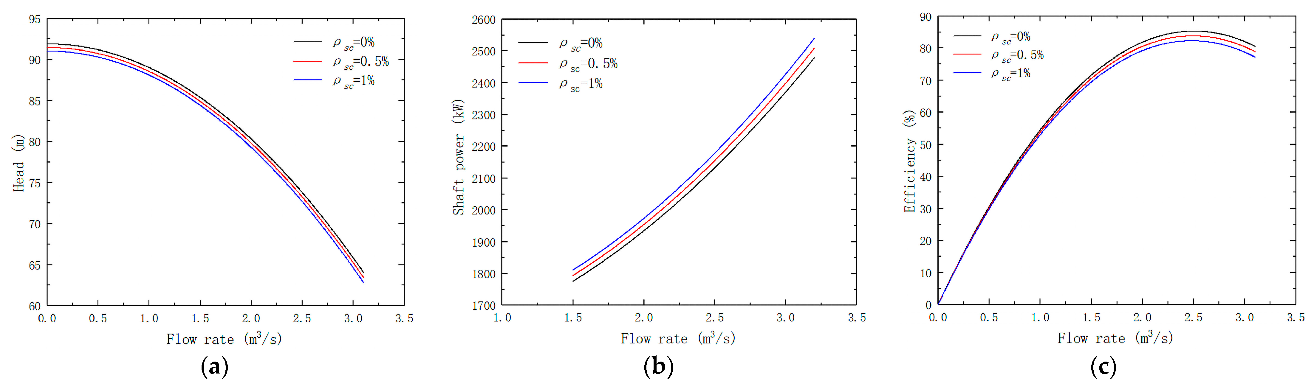
3.4.3. Characteristic Curves of Centrifugal Pump with Different Sediment Concentrations

The working parameters of the centrifugal pump (0.8 Q, Q and 1.2 Q) and sediment concentrations (ρ_sc = 0%, 0.5%, and 1%) are substituted into Equations (22)–(24). The calculation results are shown in

Table 8. Calculation results of fitting equations for sediment concentrations of 0%, 0.5%, and 1%.

ρsc (%)	Head (m)			Flow Rate (m3/s)			Shaft Power (kW)			Efficiency (%)
	0.8 Q	Q	1.2 Q	0.8 Q	Q	1.2 Q	0.8 Q	Q	1.2 Q	0.8 Q	Q	1.2 Q
0	79	75	64	2	2.5	3	1886.82	2160.08	2292.84	82	85	82
0.5	78.61	74.63	63.68	1.99	2.487	2.985	1937.13	2178.01	2377.89	80.55	83.50	80.55
1	78.23	74.26	63.36	1.98	2.474	2.969	1952.60	2195.94	2397.34	79.11	82.00	79.11

.

The curves of flow-head (Q-H), flow-shaft power (Q-N), and flow-efficiency (Q-$\eta$) are obtained under different sediment concentrations by the polynomial least-squares fitting method. The results are shown in Figure 11.

It can be seen from Figure 11 that the curves of flow-head (Q-H) and flow-efficiency (Q-η) of the centrifugal pump show overall decreasing trends with the increase of sediment concentration, while the flow-shaft power (Q-N) curve shows an overall increased trend.

4. Conclusions

In this paper, the performance of the centrifugal pump is simulated under the condition of sediment-laden flow, and then the polynomial least-squares method is used to establish fitting equations between the performance parameters of the centrifugal pump and sediment concentrations. The following conclusions can be drawn:

• The volume fraction of sediment at impeller outlet and volute wall is relatively large under the condition of sediment-laden flow, leading to the wear of blade edge and volute wall being relatively serious. Moreover, the wear of blade edge and volute wall increases with the increase of sediment concentration.
• In the impeller inlet, blade back, impeller outlet, and cochlea tongue of the centrifugal pump, there are high turbulent kinetic energy regions in different degrees under the condition of sediment-laden flow, resulting in loss of pressure and energy in the centrifugal pump. With the increase of sediment concentration, the loss of pressure and energy in the centrifugal pump also increase.
• With the increase of sediment concentration in the centrifugal pump, the head, flow rate, and efficiency of the centrifugal pump all show downward trends, while the shaft power shows a rising trend.
• The fitting equations are established between the performance parameters of the centrifugal pump and sediment concentration by the polynomial least-squares method, which can provide a simple and efficient method for the calculation of performance parameters of the centrifugal pump with different sediment concentrations. However, it can be seen from the error analysis results that, as the service time of the centrifugal pump increases, it is necessary to constantly calibrate fitting equations to ensure its calculation accuracy.

In conclusion, the fitting equations proposed in this study are proved to be applicable in a specific project. The fitted equations can be established for different projects by modifying the coefficients in the fitted function through this research method. Therefore, in order to verify the universal applicability of this method, more engineering examples are required.

References

1. Hu, C.; Zhang, X.; Zhao, Y. Cause Analysis of the Centennial Trend and Recent Fluctuation of the Yellow River Sediment Load. Adv. Water Sci. 2020, 31, 725–733. (In Chinese) [Google Scholar] [CrossRef]
2. Yue, J.; Huang, X.; Xing, X.; Zhao, L.; Kong, Q.; Yang, X.; Zhu, Y.; Zhang, J. Experimental Study on the Improvement of the Particle Gradation of the Yellow River Silt Based on MICP Technology. Adv. Eng. Sci. 2021, 53, 89–98. (In Chinese) [Google Scholar] [CrossRef]
3. Shen, Z.; Chu, W.; Li, X.; Dong, W. Sediment erosion in the impeller of a double-suction centrifugal pump—A case study of the Jingtai Yellow River Irrigation Project, China. Wear 2019, 422–423, 269–279. [Google Scholar] [CrossRef]
4. Zhang, Y.; Li, Y.; Cui, B.; Zhu, Z.; Dou, H. Numerical simulation and analysis of solid-liquid two-phase flow in centrifugal pump. Chin. J. Mech. Eng. 2013, 26, 53–60. [Google Scholar] [CrossRef]
5. Wang, K.; Pan, Y.; Zheng, J.; Li, C.; Kim, K. A Numerical Study of the Impact of Fine Sand-particles on Centrifugal Pump Working Characteristics. Chin. Rural Water Hydropower 2013, 5, 129–132. (In Chinese) [Google Scholar] [CrossRef]
6. Wang, Y.; Li, W.; He, T.; Han, C.; Zhu, Z.; Lin, Z. The effect of solid particle size and concentrations on internal flow and external characteristics of the dense fine particles solid–liquid two-phase centrifugal pump under low flow condition. Aip Adv. 2021, 11, 85309. [Google Scholar] [CrossRef]
7. Lu, J.; Du, G. Study of the Influence of Silt on the Pump Performance. J. Drain. Irrig. Mach. Eng. 2003, 21, 13–16. (In Chinese) [Google Scholar] [CrossRef]
8. Ding, H.; Visser, F.C.; Jiang, Y.; Furmanczyk, M. Demonstration and Validation of a 3D CFD Simulation Tool Predicting Pump Performance and Cavitation for Industrial Applications. J. Fluids Eng. 2011, 133, 11101. [Google Scholar] [CrossRef]
9. Buratto, C.; Pinelli, M.; Spina, P.R.; Vaccari, A.; Verga, C. CFD study on special duty centrifugal pumps operating with viscous and non-Newtonian fluids. In Proceedings of the 11th European Conference on Turbomachinery Fluid Dynamics & Thermodynamics, Madrid, Spain, 23–27 March 2015. [Google Scholar]
10. Steinmann, A.; Wurm, H.; Otto, A. Numerical and experimental investigations of the unsteady cavitating flow in a vortex pump. J. Hydrodyn. Ser. B 2010, 22, 324–329. [Google Scholar] [CrossRef]
11. Zhai, J.; Zhou, H. Model and Simulation on Flow and Pressure Characteristics of Axial Piston Pump for Seawater Desalination. Appl. Mech. Mater. 2012, 157–158, 1549–1552. [Google Scholar] [CrossRef]
12. Thakkar, S.; Vala, H.; Patel, V.K.; Patel, R. Performance improvement of the sanitary centrifugal pump through an integrated approach based on response surface methodology, multi-objective optimization and CFD. J. Braz. Soc. Mech. Sci. Eng. 2021, 43, 24. [Google Scholar] [CrossRef]
13. Wan, D.; Turek, S. An efficient multigrid-FEM method for the simulation of solid–liquid two phase flows. J. Comput. Appl. Math. 2007, 203, 561–580. [Google Scholar] [CrossRef] [Green Version]
14. Pagalthivarthi, K.V.; Visintainer, R.J. Finite Element Prediction of Multi-Size Particulate Flow through Three-Dimensional Channel: Code Validation. J. Comput. Multiphase Flows 2013, 5, 57–72. [Google Scholar] [CrossRef]
15. Kartashev, A.L.; Kartasheva, M.A.; Terekhin, A.A. Mathematical Models of Dynamics Multiphase Flows in Complex Geometric Shape Channels. Procedia Eng. 2017, 206, 121–127. [Google Scholar] [CrossRef]
16. Zhou, W.; Chai, J.; Xu, Z.; Cao, C.; Wu, G.; Yao, X. Numerical Simulation of Solid-Liquid Two-Phase Flow and Wear Prediction of a Hydraulic Turbine High Sediment Content. Exp. Tech. 2022, 1–13. [Google Scholar] [CrossRef]
17. Pathak, M. Computational investigations of solid-liquid particle interaction in a two-phase flow around a ducted obstruction. J. Hydraul. Res. 2011, 49, 96–104. [Google Scholar] [CrossRef]
18. Li, Y.; Zhu, Z.; He, Z.; He, W. Abrasion characteristic analyses of solid-liquid two-phase centrifugal pump. J. Therm. Sci. 2011, 20, 283–287. [Google Scholar] [CrossRef]
19. Huang, S.; Su, X.; Qiu, G. Transient numerical simulation for solid-liquid flow in a centrifugal pump by DEM-CFD coupling. Eng. Appl. Comp. Fluid 2015, 9, 411–418. [Google Scholar] [CrossRef] [Green Version]
20. Song, X.; Qi, D.; Xu, L.; Shen, Y.; Wang, W.; Wang, Z.; Liu, Y. Numerical Simulation Prediction of Erosion Characteristics in a Double-Suction Centrifugal Pump. Processes 2021, 9, 1483. [Google Scholar] [CrossRef]
21. Wang, B.; Zhang, H.; Deng, F.; Wang, C.; Si, Q. Effect of Short Blade Circumferential Position Arrangement on Gas-Liquid Two-Phase Flow Performance of Centrifugal Pump. Processes 2020, 8, 1317. [Google Scholar] [CrossRef]
22. Noon, A.A.; Kim, M. Erosion wear on centrifugal pump casing due to slurry flow. Wear 2016, 364–365, 103–111. [Google Scholar] [CrossRef]
23. Pagalthivarthi, K.V.; Gupta, P.K.; Tyagi, V.; Ravi, M.R. CFD Predictions of Dense Slurry Flow in Centrifugal Pump Casings. Int. J. Mech. Mechatron. Eng. 2011, 5, 538–550. [Google Scholar] [CrossRef]
24. Zhang, Y.; Li, Y.; Zhu, Z.; Cui, B. Computational analysis of centrifugal pump delivering solid-liquid two-phase flow during startup period. Chin. J. Mech. Eng. 2014, 27, 178–185. [Google Scholar] [CrossRef]
25. Fan, Y.; Gao, Z.; Wang, S.; Chen, H.; Liu, J. Evaluation of the Water Allocation and Delivery Performance of Jiamakou Irrigation Scheme, Shanxi, China. Water 2018, 10, 654. [Google Scholar] [CrossRef] [Green Version]
26. Haavisto, S.; Syrjänen, J.; Koponen, A.; Manninen, M. UDV measurements and CFD simulation of two-phase flow in a stirred vessel. Prog. Comput. Fluid Dyn. 2009, 9, 375–382. [Google Scholar] [CrossRef]
27. Pathak, M.; Khan, M.K. Inter-phase slip velocity and turbulence characteristics of micro particles in an obstructed two-phase flow. Environ. Fluid Mech. 2013, 13, 371–388. [Google Scholar] [CrossRef]
28. Zi, D.; Wang, F.; Tao, R.; Hou, Y. Research for impacts of boundary layer grid scale on flow field simulation results in pumping station. J. Hydraul. Eng. 2016, 47, 139–149. (In Chinese) [Google Scholar] [CrossRef]
29. Li, X.; Yuan, S.; Pan, Z.; Li, Y.; Yang, J. Realization and application evaluation of near-wall mesh in centrifugal pumps. Trans. Chin. Soc. Agric. Eng. 2012, 28, 67–72+293. (In Chinese) [Google Scholar] [CrossRef]
30. Kim, S.; Kojima, M. Solving polynomial least squares problems via semidefinite programming relaxations. J. Glob. Optim. 2010, 46, 1. [Google Scholar] [CrossRef] [Green Version]
31. Liang, S.; Doong, D.; Chao, W. Solution of Shallow-Water Equations by a Layer-Integrated Hydrostatic Least-Squares Finite-Element Method. Water 2022, 14, 530. [Google Scholar] [CrossRef]
32. Jiang, H. Investigation on Turbulent Flow Characteristics in a Solid-Liquid Stirred Tank. Master’s Thesis, Beijing University of Chemical Technology, Beijing, China, 2010. [Google Scholar]
33. Liu, Y.; Yang, D.; Gao, J.; Liu, C. Research on Characteristic Parameters of Jiamakou Pump Station under Condition of Sediment Flow. Water Resour. Power 2017, 35, 175–177. (In Chinese) [Google Scholar]
Figure 1. Location of Jiamakou water supply pumping station.
Energies 15 07228 g001
Figure 2. The model of fluid domain and the grid division.
Energies 15 07228 g002
Figure 3. Change curve of the head with grid number.
Energies 15 07228 g003
Figure 4. Physical picture of wear and cloud diagram of volume fraction of sediment particles: (a) physical picture of wear; (b) cloud diagram of volume fraction of sediment particles.
Energies 15 07228 g004
Figure 5. Cloud diagram of the variation of solid particle volume fraction in centrifugal pump with different sediment concentrations: (a) sediment concentration ρsc = 0.1%; (b) sediment concentration ρsc = 1%.
Energies 15 07228 g005
Figure 6. Cross-section ab solid particle volume fraction variation trend diagram: (a) sediment concentration ρsc = 0.1%; (b) sediment concentration ρsc = 1%.
Energies 15 07228 g006
Figure 7. Cloud diagram of the variation of turbulence kinetic energy in centrifugal pump with different sediment concentrations: (a) clear water; (b) sediment concentration ρsc = 0.1%; (c) sediment concentration ρsc = 1%.
Energies 15 07228 g007
Figure 8. Cross-section ab shows the variation trend of turbulence kinetic energy with different sediment concentrations.
Energies 15 07228 g008
Figure 9. The variation trend diagram of performance parameters of centrifugal pump with different sediment concentrations at the design flow rate Q.
Energies 15 07228 g009
Figure 10. Variation trend diagram of performance parameters of centrifugal pump with different sediment concentrations at 0.8 Q and 1.2 Q conditions: (a) 0.8 Q working condition; (b) 1.2 Q working condition.
Energies 15 07228 g010
Figure 11. Characteristic curves of centrifugal pump with sediment concentrations of 0%, 0.5%, and 1%: (a) flow-head (Q-H) curve; (b) flow-shaft power (Q-N) curve; (c) flow-efficiency (Q-η) curve.
Energies 15 07228 g011