Abstract
Accurate and reasonable matching design is a current and difficult point in electric vehicle research. This paper presents a parameter optimization method for the power system of a medium-sized bus based on the combination of the orthogonal test and the secondary development of ADVISOR software. According to vehicle theoretical knowledge and the requirements of the vehicle power performance index, the parameters of the vehicle power system were matched and designed. With the help of the secondary development of MATLAB/Simulink and ADVISOR software, the modeling of the key parts of the vehicle was carried out. Considering the influence of the number of battery packs, motor power model, wheel rolling resistance coefficient, and wind resistance coefficient on the design of the power system, an L9 (34)-type orthogonal table was selected to design the orthogonal test. The dynamic performance and driving range of the whole vehicle were simulated using different design schemes, and the accuracy of the simulation results was verified by comparing and analyzing the simulation images. The results demonstrated that in the environment where the wind resistance coefficient was 0.6 and the wheel rolling resistance coefficient was 0.009, with 240 sets of lithium batteries (battery energy, 264 kW h; battery capacity, 100 Ah) as the power source, the pure electric medium-sized bus equipped with the PM165 permanent magnet motor (rated power, 60 kW; rated torque, 825 N m) could obtain the best power performance and economic performance. The research content of this paper provides a certain reference for the design of shuttle buses for Nantong’s bus system, effectively reduces the testing costs of the vehicle development process, and provides a new idea for the power system design of pure electric buses.
1. Introduction
The development of the traditional automobile industry is currently limited by the shortage of resources [1] and environmental pollution [2]. Under the concept of sustainable development, new-energy vehicles have gradually gained public recognition. New-energy vehicles are mainly divided into three categories, namely, hybrid vehicles, pure electric vehicles, and fuel-cell vehicles [3]. After years of research and development, pure electric buses have taken a dominant position in the field of passenger cars. With the advantages of no pollution, low noise, high energy efficiency, and convenient maintenance, they have been popularized in various cities and have gradually replaced traditional fuel buses. They have achieved great advantages in protecting the environment, improving the country’s energy structure, and reducing urban noise pollution [4].
However, there are still some problems in the development of the power system of the pure electric bus. (1) The selection of the motor [5]: For example, when the traffic is congested, the pure electric vehicle has a smaller loss than the fuel vehicle. However, due to the characteristics of the motor’s low-speed constant torque and high-speed constant power characteristics, when driving at high speed, the electric vehicle’s energy consumption growth is much larger than that of conventional vehicles [6]. (2) The selection of power batteries [7]: The selection of batteries directly affects the cruising range [8] and safety of buses. At present, lithium iron phosphate batteries and ternary batteries occupy the power battery market for pure electric buses. Both have certain problems. The former has good cycle stability but large mass and low energy density. The latter has high energy density but poor safety. It is easy to spontaneously ignite when the temperature is high, and it is difficult to control [9].
Many researchers have studied the power system of pure electric buses. Hu et al. [10] developed the power distribution control strategy of the dual-motor coupling mode considering the dynamic characteristics of the motor by constructing a vehicle model including the motor dynamic control model and simulated it in the MATLAB platform. The results showed that the established dynamic model of the motor was closer to the actual operating conditions. The control strategy effectively reduced the power demand of the electric drive system, reduced the energy consumption of the electric drive system, and extended the vehicle mileage. Vora et al. [11] proposed a novel framework that enables the parametric design optimization of hybrid electric vehicles, taking into account battery degradation and its impact on the vehicle life cycle. The framework captures the impact of battery degradation on fuel consumption and battery replacement by integrating a battery model capable of predicting degradation and performance degradation into drive cycle simulations. Raga et al. [12] analyzed the different factors that affect the optimal design of a power system (including the minimum power provided by the fuel cell, the storage of recovered energy in the regenerative braking stage, the battery technology, and the change in the maximum charging state of the battery) and analyzed how these design factors affect the quality, volume, and cost of the optimal distribution architecture, as well as how to consider these factors in the design. Hoshing et al. [13] compared the life-cycle cost of series and parallel architectures for PHEVs, saving fuel costs and enabling a faster return on investment for transit bus scenarios compared with medium-duty trucks, driving the early viability of transit bus applications. Soltani et al. [14] studied the effectiveness of the hybrid energy storage system in protecting the battery from high power loss during charging and discharging, reducing the negative impact of power peaks related to urban driving cycles, and improving the battery life by 16%. Jin et al. [15] evaluated state-of-the-art methods in Li-ion battery degradation models, including accuracy, computational complexity, and ease-of-control algorithm development. Based on a comparison of simulation results and experimental data, key differences in aging factors captured by each model were summarized. However, there is a problem in these research processes, that is, the fact that they only considered the influence of single factors, such as battery or motor, on the design of the power system, without considering whether the matching of battery, motor, and other components was the best, which may have led to the dynamic performance of the vehicle not being fully reflected. Therefore, the analysis of the selection and matching of different components plays an important role in the design of pure electric buses.
The orthogonal test is another design method to study multiple factors and levels. It selects some representative points from the comprehensive test according to orthogonality. These representative points have the characteristics of “uniform dispersion, neat and comparable”. Orthogonal test design is the main method in fractional factorial design. Xu et al. [16] optimized the spin-forming parameters of bimetallic composite pipes using the finite element method and the experimental method and analyzed the torque and residual contact pressure in the forming process. Through the orthogonal test method to optimize the spinning process parameters of the bimetal composite pipe and through the deep drawing experiment of the composite pipe, the accuracy of the numerical simulation value was verified. Quan et al. [17] used the orthogonal experimental design method combining experiments and numerical calculations to optimize the design structure of a vortex pump impeller. Through an orthogonal experimental design, the design cycle of the vortex pump could be effectively shortened; the design level of the vortex pump could be improved; and a hydraulic model with superior performance could be obtained. Yu et al. [18] studied the effects of load, frequency, duration, and concentration on the friction properties of additives on an SRV reciprocating wear tester using an orthogonal experimental design. This paper was not only aimed at the single factor of battery or motor but also at the multi-factor and multi-level research of different batteries, motors, and other influencing factors. Therefore, the orthogonal test was very consistent with the design of the experimental scheme.
ADVISOR is a series of models, data, and script files in the MATLAB and Simulink software environment. It can quickly analyze the fuel savings, power, and emissions of traditional vehicles, pure electric vehicles, and hybrid electric vehicles using the parameters of various parts of the vehicle under the given road cycle conditions. Sun et al. [19] used ADVISOR and iSIGHT software to jointly optimize the transmission ratio and used ADVISOR simulation software to analyze the savings and power of the optimized transmission ratio. The optimized pure electric passenger vehicle achieved a balance between power and economic performance, thus giving play to its performance advantages. Wang et al. [20] established the energy model of a vehicle system using ADVISOR and MATLAB software. An energy control strategy for the dynamic wireless charging of electric vehicles was designed. The influence of dynamic wireless power transmission on energy storage system loss and electric vehicle range under different operating scenarios and different battery minimum charging states was studied. Sun et al. [21] selected configuration parameters such as vehicle body, battery, tires, and transmission in ADVISOR for simulation and selected vehicle mass, rolling resistance coefficient, and auxiliary power as control variables to conduct a cost–benefit analysis based on the vehicle’s full life-cycle mileage, so as to reduce the short-term profit limit of optimization evaluation, which has practical guiding significance for the formulation of an energy optimization scheme for electric commercial vehicles. The biggest feature of ADVISOR software is that the simulation model and software source code are completely open all over the world and can be downloaded free of charge from the website. On the basis of the original simulation model, researchers can modify or reconstruct some simulation models and adjust or redesign the control strategy as needed to make it closer to the actual situation, and the simulation results are more reasonable. Through the secondary development of the battery model and motor model in ADVISOR, this paper made the simulation process more reasonable and more practical.
This paper combined MATLAB/Simulink and ADVISOR software to analyze and model the whole vehicle, battery, motor, etc., of a medium-sized bus [22]. Around the needs of the actual vehicle model [23], according to the orthogonal test table, multiple groups of combined parameters, such as different numbers of battery packs, motor power models, wheel rolling resistance coefficients, and wind resistance coefficients, were determined. The influence of different combined parameters on the power performance and economic performance of a pure electric medium-sized bus was simulated and analyzed [24]. The optimization scheme of the power system of an electric bus was selected through comparison, and the feasibility of the optimization scheme was verified. It can provide a certain reference for the design of shuttle buses for Nantong’s public transport system and provides a new idea for the design of the power system of a pure electric bus. Figure 1 presents a flow chart showing the structure of this paper.
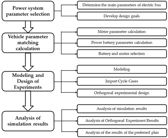
Figure 1.
Structure flow chart.
2. Parameter Selection of Pure Electric Bus Power System
2.1. Selection of Main Parameters and Performance Indicators
The authors’ first work unit has cooperated with Nantong’s public transport company for many years. As early as 2013, we carried out a cooperative research study on the comprehensive operation and management platform of multi-model new-energy vehicles [25] and cooperated in the demonstration, promotion, and application of new-energy vehicles in Nantong. Because many subway lines are about to be opened in Nantong, the bus lines in Nantong also need to be adjusted accordingly, and the length of the bus lines needs to be appropriately shortened. Therefore, it is necessary to design an electric bus power system suitable for short haul. According to the actual needs of Nantong City’s public transportation system and the market positioning of an electric bus, after referring to the design of similar vehicles on the market, we determined the pure electric vehicle power system with an on-board battery pack as the power and a motor as the driving device [26]. The design of the electric bus should meet the relevant requirements of the power performance and driving range of the whole vehicle [27,28]. See Table 1 and Table 2 for vehicle parameters, dynamic performance, and economical parameters.

Table 1.
Vehicle parameters of pure electric vehicle.
Table 2.
Power performance requirements for pure electric vehicles.
2.2. Vehicle Parameter Matching Calculation
2.2.1. Motor Parameter Calculation
- (1)
- Determination of peak power and rated power
The power matching of the motor of a pure electric vehicle directly affects the dynamic performance of the vehicle [29]. Matching reasonable motor power not only can extend the driving distance of the car, but it can also improve energy utilization. In addition, the peak power of the motor must meet the requirements corresponding to the maximum grade and acceleration time.
Under different driving conditions of the vehicle, the vehicle driving power balance equations are represented by Formulas (1)–(3) [30]:
where is the motor power determined according to the maximum vehicle speed; is the motor power determined according to the maximum grade; is the motor power determined according to the acceleration time; and is the mass of the medium-sized passenger car, and its value can be slightly larger due to the calculation error. According to the expected simulation target, we took the vehicle mass as 9000 kg; , the maximum speed, as 70 km/h; , the mechanical efficiency, as 0.9; , the wheel rolling resistance coefficient, as 0.009; , the acceleration of gravity, as 9.8 m/s²; , the wind resistance coefficient, as 0.7; , the windward area, according to the width and height of a medium-sized bus, as 8.55 m²; , the speed at the maximum climbing degree, as 20 km/h; , the maximum angle; , the car rotating-mass conversion factor, as 1.1; , the acceleration time, as 25 s; and , the final speed, as 50 km/h.
The power of the motor must meet the power requirements of the vehicle, that is, the above three formulas must be satisfied at the same time. The rated power was 47.11 kW, as calculated from the maximum vehicle speed. The calculated was 94.16 kW, and was 157.96 kW, as obtained from the acceleration performance requirements. The car lasts for a longer time at top speed. We took the maximum value of the acceleration time and the maximum grade result as the maximum power of the electric vehicle motor.
- (2)
- Determination of peak speed and rated speed
The formulas of rated speed and peak speed of the motor are shown in Equations (4) and (5) [31]:
where is the reduction ratio of the electric vehicle, which can be 3.5~5; is the tire radius (Michelin tires were selected in the used software), and the value was 0.282 m; and is 2~4.
- (3)
- Determination of peak torque and rated torque
The rated power and rated speed of the motor determine the rated torque of the motor [32]; then, the rated torque and maximum torque of the motor are expressed as:
where is the rated torque of the motor, is the rated speed of the motor, is the maximum torque of the motor and is 2–3.
From the calculation results, the motor parameters are shown in Table 3.
Table 3.
Motor parameters.
2.2.2. Calculation of Power Battery Parameters
The rated power required by the motor according to the maximum driving speed of the car can be calculated as shown in formula (9) [33]:
By substituting the data, we obtained = 23.17 kW.
The energy required by the battery based on the range of the car can be determined as:
where is the cruising range (we took 200 km) and is the constant speed (we took 50 km/h).
By substituting the data, we obtained = 92.68 kJ.
where is the actual energy of the battery pack, is the capacity of the battery, is the rated working voltage of the battery pack (the value taken was 240 V) and is the depth of discharge. Since deep discharge causes irreparable damage to the battery, the depth of discharge was selected as 80%. In order to meet the requirements of the car, it is necessary to make the battery pack meet > ; then, > (92.68 × 1000/240/0.8) = 263.3 kWh.
2.2.3. Selection of Battery and Motor
Power battery is an important part of pure electric vehicle power systems [34], among which the lithium iron phosphate battery has become the first choice for passenger cars due to its advantages of high safety, low cost, high energy density, and power density. Most of the electric vehicles on the market, such as Yutong Bus (Zhengzhou, China), Xiamen King-long (Xiamen, China), and Foton AUV (Beijing, China), are equipped with permanent magnet synchronous motors [35]. To sum up, in this design, a lithium iron phosphate battery with a battery density of 210 Wh/kg was selected as the power source of the medium-sized bus. The cell voltage of the battery pack was 11 V; the battery capacity was 100 Ah; and the battery energy density was 210 Wh/kg.
The single mass of 240 groups, 280 groups, and 320 groups of battery packs could be calculated as 5.25 kg (rated voltage × amp-hours/energy density), and the battery power values were: 264 kWh, 308 kWh, and 352 kWh (the number of battery packs × amp-hours × rated voltage). At the same time, permanent magnet synchronous motors PM150, PM165, and PM180 were selected as drive motors to meet their power and economic performance requirements. The above selection of battery and motor parameters lay the foundation for the subsequent orthogonal experiments.
Table 4.
Battery parameters.
Table 5.
Motor parameters.
3. Dynamic System Modeling and Orthogonal Experimental Design
3.1. Vehicle Model
The power system of the electric bus was optimized using simulation platform ADVISOR [36]. In the Simulink environment, through the simulation integrated environment, the vehicle controller model was established, and the simulation was carried out on the ADVISOR platform. The top-level model is shown in Figure 2. First, the speed curve provided by the cycle condition module (drive cycle) is used as the input source; the required driving force is calculated in the vehicle dynamics model; the corresponding torque and speed are requested from the wheel and axle module; and the required driving force is calculated in the vehicle dynamics model. The backward path is gradually transmitted to the final drive, gear box, motor controller, etc.; then, the power is distributed to the battery module (energy storage) through the control strategy module (insight). The battery pack module has to calculate the actual power that can be provided, provide the power source, catch up with the target speed of the working condition, realize the purpose of exerting the maximum power of the car, and calculate the actual speed that the car can achieve; thus, the calculation of the backward path is completed.
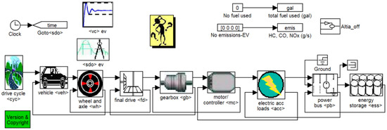
Figure 2.
Top-level module of vehicle model simulation.
3.2. Battery Model
Figure 3 presents the top-level model diagram of the battery module, which mainly included five modules. Module 1 (pack Voc, Rint): The model is an equivalent circuit of an open-circuit voltage (Voc) and an equivalent internal resistance (Rint). When calculating Rint, there are two functions: one is the charge internal resistance function (Rdis), and the other is the discharge internal resistance function (Rchg). Module 2 (compute current): Module 2 uses Voc and Rint of module 1 and the actual power (Pa) of module 4 to solve the current of the battery equivalent circuit. Module 3 (SOC algorithm): This model calculates the power consumption of the battery and the remaining SOC value through the battery current. Module 4 (limit power): This is the limit module of the maximum power that the battery can provide. Module 5 (ess_tmp): The thermal model of the battery is used to monitor the temperature of the battery.
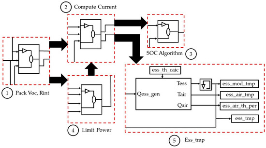
Figure 3.
Top-level model diagram of battery module: (1) pack Voc, Rint, (2) compute current, (3) SOC algorithm, (4) limit power, and (5) ess_tmp.
Because there is no lithium iron phosphate battery model with a battery density of 210 Wh/kg in ADVISOR, this paper conducted the secondary development of the battery model using software and established a new lithium iron sulfate battery model by modifying the M file. Figure 4 presents a graph showing the relationship between the battery SOC and current.
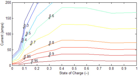
Figure 4.
Battery current diagram.
3.3. Motor Model
Figure 5 presents the top-level model diagram of the motor module. The simulation model of the drive motor mainly included the request input power calculation module, the motor actual output torque and speed calculation module, and the motor temperature calculation module in the lower right corner. The upper part of the power, torque, and speed calculation module is necessary to select the torque and speed to be output according to the working conditions, and the lower part is necessary to assume the torque and speed that should be output. If the requested speed is less than the maximum speed, the actual speed is the requested speed; otherwise, the actual speed is the maximum speed.

Figure 5.
Top-level model diagram of the motor module.
Here, we mainly introduce the model operation process of the first half, as shown in Figure 6. First, according to the working conditions, the torque and speed requested by the wheel (torque and speed req’d at rotor), the requested motor torque (mc_trq_out_r), the speed (mc_spd_out_r), and the perform motor speed estimator and motor limit torque estimation (enforce torque limit), and the results are obtained by looking up the table in the motor/controller input power map (W). The actual output power (req’d motor input power (W)) and the corresponding torque (N-m drive torque per W input) are finally sent to the power battery model and MATLAB workspace through the motor controller logic interface.

Figure 6.
Model flow diagram of the first half.
Because there is no permanent magnet synchronous motor model that meets the design requirements in ADVISOR, this paper conducted the secondary development of the motor model using software and established a new permanent magnet synchronous motor model by modifying the M file. Figure 7 presents a diagram showing the relationship between the motor speed and torque.

Figure 7.
Motor torque diagram.
3.4. Cyclic Conditions
According to “GB/T 18386-2017 Test Method for Electric Vehicle Energy Consumption and Driving Range”, the loop conditions of typical Chinese cities were selected as the conditions for the cycle calculation of operating conditions [37]. Table 6 shows the statistical characteristics of the cycle of public transport (CLTC) data of typical cities in China, and Figure 8 shows the driving condition diagram.
Table 6.
CLTC data in typical Chinese cities.
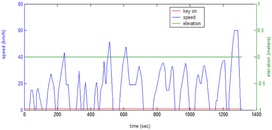
Figure 8.
CLTC-C driving condition diagram.
3.5. Orthogonal Experimental Design
In the experiments, there were four factors to be investigated (number of battery packs, motor power type, wheel rolling resistance coefficient, and wind resistance coefficient), where each factor had three levels, and the L9 (34) orthogonal table was selected [38] to schedule the experiments. The factor levels of the test are shown in the orthogonal parameter table in Table 7, and the table header design and the combination of each factor level are shown in the orthogonal test in Table 8. As can be seen in the table, we only needed to perform nine sets of experiments according to the orthogonal table.
Table 7.
Orthogonal parameter table.
Table 8.
Orthogonal experimental table.
4. Simulation Results and Discussion
4.1. Dynamic Simulation Results
According to the nine schemes obtained from the orthogonal experiments, the number of battery packs, motor power model, wheel rolling resistance coefficient, and wind resistance coefficient were selected in ADVISOR, and the CLTC working condition was selected. According to the calculation results in the second section, the depth of discharge ε_ess was taken as 80%, and the number of cycles of the working condition was selected to make the SOC of the battery ≥ 20%. The speed range was 0~50 km/h, and the climbing speed was set to 12.4 mph (equivalent to 20 km/h). The obtained simulation results are shown in Figure 9, Figure 10, Figure 11, Figure 12, Figure 13, Figure 14, Figure 15, Figure 16 and Figure 17, and the simulation results are sorted and shown in Table 9. The application and detailed discussion of simulation results are reported in the following paragraphs.

Figure 9.
Simulation results of experiment 1.

Figure 10.
Simulation results of experiment 2.
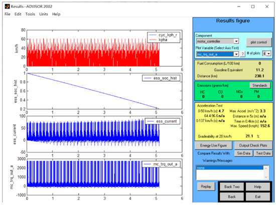
Figure 11.
Simulation results of experiment 3.

Figure 12.
Simulation results of experiment 4.
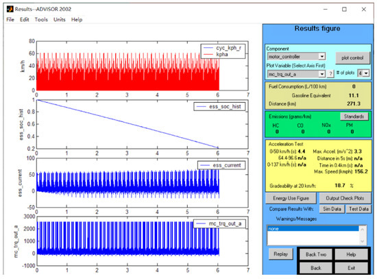
Figure 13.
Simulation results of experiment 5.

Figure 14.
Simulation results of experiment 6.
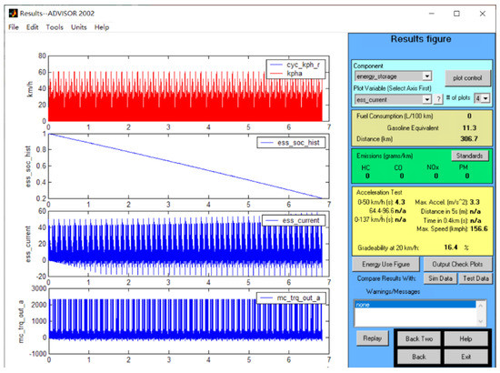
Figure 15.
Simulation results of experiment 7.

Figure 16.
Simulation results of experiment 8.
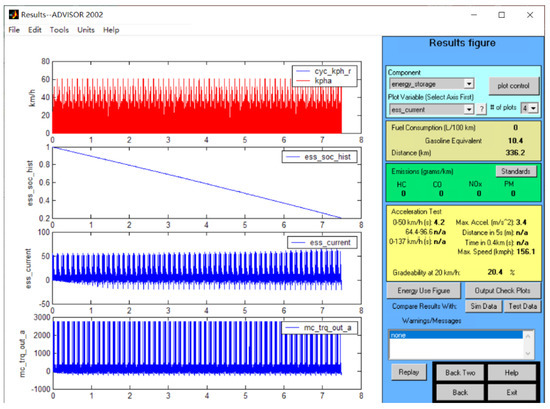
Figure 17.
Simulation results of experiment 9.
Table 9.
Dynamic simulation test results.
4.1.1. Simulation Results Diagram of Experiment 1
The results of Experiment 1 are shown in Figure 9.
4.1.2. Simulation Results Diagram of Experiment 2
The results of Experiment 1 are shown in Figure 10.
4.1.3. Simulation Results Diagram of Experiment 3
The results of Experiment 1 are shown in Figure 11.
4.1.4. Simulation Results Diagram of Experiment 4
The results of Experiment 1 are shown in Figure 12.
4.1.5. Simulation results diagram of experiment 5
The results of Experiment 1 are shown in Figure 13.
4.1.6. Simulation Results Diagram of Experiment 6
The results of Experiment 1 are shown in Figure 14.
4.1.7. Simulation Results Diagram of Experiment 7
The results of Experiment 1 are shown in Figure 15.
4.1.8. Simulation Results Diagram of Experiment 8
The results of Experiment 1 are shown in Figure 16.
4.1.9. Simulation Results Diagram of Experiment 9
The results of Experiment 1 are shown in Figure 17.
4.1.10. Summary of Dynamic Simulation Test Results
The dynamic simulation test results are sorted and shown in Table 9.
4.2. Economic Simulation Results
4.2.1. Battery Parameter Query
In the battery module, we opened (pack Voc, Rint) in the battery module, added the To Workspace module, and changed its name to open_voltage, as shown in Figure 18, that is, the data of the open circuit voltage could be sent to the MATLAB workspace. Then, we loaded the data retained by the simulation, found the variables ess_current and open_voltage, and counted the data in the Excel sheet, as shown in Figure 19 (the figure shows an example of a screenshot of some test parameters).

Figure 18.
Secondary development diagram of battery model.
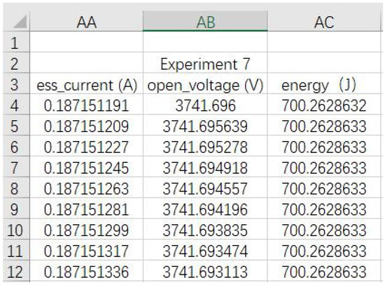
Figure 19.
Partial screenshot of test parameters.
4.2.2. Battery Energy Conversion
The integral operation of the power (P = UI) during the period from the initial time, t0, to the end of the driving time, tm, that is, the instantaneous power per second, was calculated using Excel data processing and summed to obtain the energy consumed by the car; finally, the power consumption of the medium-sized passenger car could be simulated through the calorific value conversion. The formula for calculating the energy consumption of a vehicle is shown in Equation (11):
The statistical results are shown in Table 10 below, where “−” in the table indicates energy loss.
Table 10.
Summary of energy consumption.
4.3. Orthogonal Experimental Results and Analysis
4.3.1. Summary of Experimental Results
First of all, according to the results of the dynamic simulation and economic simulation, the data were summarized to facilitate the selection of the nine schemes. The summary results are shown in Table 11.
Table 11.
Orthogonal experimental results.
4.3.2. Conversion of Membership Degrees
For orthogonal experiments with multiple indicators, the corresponding indicators are usually converted into their membership degrees using the comprehensive scoring method [39]:
where Mi represents the index membership degree, represents the index value, represents the minimum value of the index and represents the maximum value of the index.
We converted the five indicators of the test results into their membership degrees and judged the pros and cons of the indicators according to their subordination. The first four indicators were positively correlated with vehicle performance, while the last indicator was negatively correlated; that is, the greater the indexes of maximum cruising range, acceleration time, grade, and top speed were, the better the vehicle’s dynamic performance was. However, regarding the economic indicator of the pure electric bus, the power consumption per 100 km, the lower the energy consumption was, the higher the saving was. In order to obtain the correct comprehensive evaluation of dynamic performance and economic performance, this paper converted the power consumption per 100 km into the negative index and substituted it into the above formula for calculation. The membership calculation results are shown in Table 12.
Table 12.
Membership degree calculation results.
4.3.3. Comprehensive Scoring Method
A comprehensive scoring method was used to assign a weight to each indicator score. The formula is as follows:
where represents the maximum cruising range, represents the 0~50 km/h acceleration time, represents climbing at 20 km/h, represents the maximum speed and represents the power consumption. The comprehensive scores and the calculation parameter results are shown in Table 13.
Table 13.
Comprehensive scores and calculation parameter results.
4.3.4. Determining Preferred Options
According to the results obtained using the comprehensive scoring method, K1, K2, K3, and range R were calculated, and the primary and secondary relationships of each factor were further determined; finally, the preferred solution was obtained. The results are shown in Table 14.
Table 14.
Analysis table of experimental results.
According to the calculation, the primary and secondary relationships of each factor were C > D > B > A, and the optimal solution, C1D1B2A1, was obtained; that is, the number of battery packs was 240; the motor was PM165; the wind resistance coefficient was 0.6; and the wheel rolling resistance coefficient was 0.009.
4.4. Checking and Analysis of Preferred Schemes
4.4.1. Checking of Preferred Schemes
This scheme did not exist in the orthogonal test and needed to be re-tested. Figure 20 shows the simulation results.
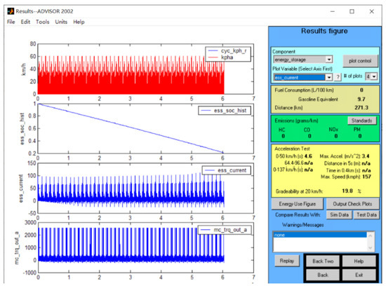
Figure 20.
Multi-condition simulation results.
4.4.2. Analysis of Preferred Schemes
It can be seen from this that the speed of the car changed frequently during driving, including driving states such as idling, starting, accelerating, and braking. During the driving process of the car, when the driving time increased, the state of charge (SOC) of the battery gradually decreased and stabilized with time and finally tended to 0.2, but the curve slightly fluctuated during the change, indicating that energy recovery played a role when the car was braking. The battery stopped discharging; the car reached the maximum cruising range; the discharge was normal, and the discharge depth was 80%. The output torque of the drive motor changed with the driving time of the car. The torque change can be seen from the curve. The positive and negative values of the torque reflect the running state of the motor.
According to the design goals, the maximum driving distance had to be ≥250 km; the 20 km/h grade had to be ≥15%; the acceleration time from 0 to 50 km/h had to be ≤5 s; the maximum speed had to be ≥150 km/h; and the power consumption per 100 km had to be ≤80 kWh/100 km. The optimization results showed that the maximum and minimum cruising distance was 271.3 km > 250 km, which was 8.52% higher than the design target. The acceleration time from 0 to 50 km/h was 4.6 s < 5 s, which was 8% lower than the design target. The gradient was 19.8% > 15%, which was 32% higher than the design target. The maximum speed was 156.4 km/h > 150 km / h, which was 4.67% higher than the design target. The power consumption per kilometer was 76.4 kWh/100 km < 80 kWh/100 km, which was 4.5% lower than the design target. The above indexes met the dynamic performance requirements, and the economic performance was more reasonable. All indicators were ideal, met the expected design requirements, and could meet the use of the model. Therefore, the simulation of a medium-sized bus achieved good results. The comparative analysis of the preferred scheme and design objectives is shown in Table 15.
Table 15.
Comparative analysis of performance and design objectives of optimization scheme.
4.5. Vehicle Driving Conditions under Different SOCs
As shown in Figure 21, under different initial SOCs, the actual AC speed that the vehicle could reach was completely consistent with the cycle speed curve, which indicated that the motor and battery under this scheme could be well compatible, so that the vehicle had good power performance to meet the needs of speed change under working conditions.
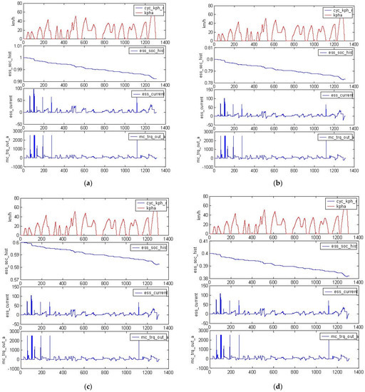
Figure 21.
Simulation results of a single case with different initial SOCs: (a) SOC = 1, (b) SOC = 0.8, (c) SOC = 0.6, and (d) SOC = 0.4.
5. Conclusions
The main purpose of this paper was to reduce the testing costs of the whole shuttle bus development of Nantong’s public transportation system through simulation experiments and to provide new ideas for the power system design of pure electric buses. This paper presents an optimization method for the power system of pure electric buses based on the combination of orthogonal experiments and software secondary development. Based on the modeling of a pure electric bus, the basic parameters of the vehicle were determined; the vehicle power system scheme was simulated and analyzed; and the power system design scheme with the best power performance and economic performance was optimized, which could effectively reduce the testing costs in the process of vehicle development. The main conclusions were as follows:
- (1)
- The main parameters of the bus and the expected performance indicators were determined. According to market research, the parameters of the battery cells and the selection of the motor were determined, and the parameters of 240, 280, and 320 sets of lithium iron phosphate batteries were selected by calculating the battery capacity and motor power, along with the PM150, PM165, and PM180 series permanent magnet synchronous motor parameters;
- (2)
- Based on the secondary development of ADVISOR software, the models of each module of the power system were constructed. Taking China’s typical urban bus cycle (CLTC) as the experimental cycle, different battery pack numbers (a), motor powers (b), wind resistance coefficients (c), and wheel rolling resistance coefficients (d) were selected as the influencing factors in the orthogonal experiments. Each factor was set at three levels to complete the simulation analysis of the power performance and economic performance of the pure electric bus;
- (3)
- According to the orthogonal test and comprehensive scoring method, the design scheme of the pure electric medium-sized bus was optimized to run in the environment of 0.6 (C1) and 0.009 (D1) with 240 groups of lithium batteries (A1) (rated voltage, 220 V; battery capacity, 100 Ah; battery power, 264 kW h; battery mass, 1260 kg) as the power source, equipped with permanent magnet motor PM165 (B2) (rated voltage, 220 V; rated power, 60 kW; rated torque, 825 N m; rated speed, 1450 r/min; motor mass, 162 kg). Its performance indicators were as follows: the maximum cruising range was 271.3 km; the acceleration time from 0 to 50 km/h was 4.6 s; the gradient was 19.8%; and the maximum speed was 156.4 km/h.
The sample size of the experiments in this paper was moderate, and the sample size could continue to be expanded. In addition, there was a lack of appropriate bench experiments to verify the experimental results. According to the research contents and literature references of this paper [40,41], four suggestions are put forward for future work: (1) increase in the number of samples and experiments; (2) appropriate increase in bench experiments; (3) attempts to optimize the simulation results using smart algorithms, such as genetic algorithms; (4) analyses of the costs of vehicle design and vehicle emissions.
Author Contributions
Conceptualization, X.W.; methodology, X.W.; software and validation, P.Y. and Y.Z. (Yujie Zhang); formal analysis, X.W. and P.Y., investigation, P.Y. and S.L.; resources, H.N. and Y.Y.; data curation, P.Y.; writing—original draft preparation, P.Y; writing—review and editing, X.W. and Y.D.; visualization, Y.Z. (Yujie Zhang); supervision, Y.Z. (Yu Zhu); project administration, Y.D. and Y.Y.; funding acquisition, H.N. and Y.Y. All authors have read and agreed to the published version of the manuscript.
Funding
This research study was funded by National Natural Science Foundation of China (grant Nos. 51905361 and 51876133) and Jiangsu Provincial Key Research and Development Program of China (grant No. BE2021065).
Institutional Review Board Statement
Not applicable.
Informed Consent Statement
Not applicable.
Data Availability Statement
Not applicable.
Acknowledgments
This research study was funded by National Natural Science Foundation of China (grant Nos. 51905361 and 51876133) and Jiangsu Provincial Key Research and Development Program of China (grant No. BE2021065) and is a project funded by Priority Academic Program Development of Jiangsu Higher Education Institutions (PAPD). Thanks to Nantong Public Traffic General Company for providing relevant experimental data for this article. The authors would like to thank the anonymous reviewers for their reviews and comments.
Conflicts of Interest
The authors declare no conflict of interest.
Abbreviations
| Parameter | Meaning Represented |
| whole-vehicle quality | |
| rotating-mass conversion factor | |
| wheelbase | |
| air drag coefficient | |
| windward area | |
| rolling resistance coefficient | |
| electric motor power based on top speed | |
| motor power according to maximum grade | |
| motor power according to acceleration time | |
| motor peak speed | |
| motor rated speed | |
| electric vehicle reduction ratio | |
| tire radius | |
| motor rated torque | |
| motor peak torque | |
| maximum speed | |
| mechanical efficiency | |
| gravitational acceleration | |
| speed at maximum grade | |
| maximum angle | |
| acceleration time | |
| final velocity | |
| energy required by battery pack | |
| cruising range | |
| constant driving speed | |
| battery pack actual energy | |
| battery capacity | |
| rated working voltage of battery pack | |
| depth of discharge | |
| index membership degree | |
| index value | |
| maximum value of index | |
| minimum value of index | |
| maximum cruising range | |
| 0~50 km/h acceleration time | |
| climbing at 20 km/h | |
| maximum speed | |
| power consumption |
References
- Krawczyk, P.; Kopczyński, A.; Lasocki, J. Modeling and Simulation of Extended-Range Electric Vehicle with Control Strategy to Assess Fuel Consumption and CO2 Emission for the Expected Driving Range. Energies 2022, 15, 4187. [Google Scholar] [CrossRef]
- Neugebauer, M.; Zebrowski, A.; Esmer, O. Cumulative Emissions of CO2 for Electric and Combustion Cars: A Case Study on Specific Models. Energies 2022, 15, 2703. [Google Scholar] [CrossRef]
- Wang, X.X.; Zhang, Y.J.; Zhu, Y.; Lv, S.S.; Ni, H.J.; Deng, Y.L.; Yuan, Y.N. Effect of Different Hot-Pressing Pressure and Temperature on the Performance of Titanium Mesh-Based MEA for DMFC. Membranes 2022, 12, 431. [Google Scholar] [CrossRef] [PubMed]
- Kernytskyy, I.; Yakovenko, Y.; Horbay, O.; Ryviuk, M.; Humenyuk, R.; Sholudko, Y.; Voichyshyn, Y.; Mazur, Ł.; Osiński, P.; Rusakov, K.; et al. Development of comfort and safety performance of passenger seats in large city buses. Energies 2021, 14, 7471. [Google Scholar] [CrossRef]
- Geng, H.; Zhang, X.; Yan, S.; Zhang, Y.; Wang, L.; Han, Y.; Wang, W. Magnetic Field Analysis of an Inner-Mounted Permanent Magnet Synchronous Motor for New Energy Vehicles. Energies 2022, 15, 4074. [Google Scholar] [CrossRef]
- Dziechciarz, A.; Popp, A.; Marțiș, C.; Sułowicz, M. Analysis of NVH Behavior of Synchronous Reluctance Machine for EV Applications. Energies 2022, 15, 2785. [Google Scholar] [CrossRef]
- Barbieri, M.; Ceraolo, M.; Lutzemberger, G.; Scarpelli, C. An Electro-Thermal Model for LFP Cells: Calibration Procedure and Validation. Energies 2022, 15, 2653. [Google Scholar] [CrossRef]
- Szumska, E.M.; Jurecki, R.S. Parameters influencing on electric vehicle range. Energies 2021, 14, 4821. [Google Scholar] [CrossRef]
- Wang, X.X.; Liu, S.R.; Zhang, Y.J.; Lv, S.S.; Ni, H.J.; Deng, Y.L.; Yuan, Y.N. A Review of the Power Battery Thermal Management System with Different Cooling, Heating and Coupling System. Energies 2022, 15, 1963. [Google Scholar] [CrossRef]
- Hu, J.J.; Jia, M.X.; Xiao, F.; Fu, C.Y.; Zheng, L.L. Motor vector control based on speed-torque-current map. Appl. Sci. 2019, 10, 78. [Google Scholar] [CrossRef]
- Vora, A.; Jin, X.; Hoshing, V.; Guo, X.F.; Shaver, G.; Tyner, W.; Holloway, E.; Varigonda, S.; Kupe, J. Simulation framework for the optimization of hev design parameters: Incorporating battery degradation in a lifecycle economic analysis. IFAC-Pap. 2015, 48, 195–202. [Google Scholar] [CrossRef]
- Raga, C.; Barrado, A.; Lazaro, A.; Martin-Lozano, A.; Quesada Isabel, Z.P. Influence of the main design factors on the optimal fuel cell-based powertrain sizing. Energies 2018, 11, 3060. [Google Scholar] [CrossRef]
- Hoshing, V.; Vora, A.; Saha, T.; Jin, X.; Shaver, G.; Wasynczuk, O.; García, R.E.; Varigonda, S. Comparison of economic viability of series and parallel PHEVs for medium-duty truck and transit bus applications. Proc. Inst. Mech. Eng. Part D J. Automob. Eng. 2020, 234, 2458–2472. [Google Scholar] [CrossRef]
- Soltani, M.; Ronsmans, J.; Kakihara, S.; Jaguemont, J.; Bossche, P.V.D.; Mierlo, J.V.; Omar, N. Hybrid battery/lithium-ion capacitor energy storage system for a pure electric bus for an urban transportation application. Appl. Sci. 2018, 8, 1176. [Google Scholar] [CrossRef]
- Jin, X.; Vora, A.; Hoshing, V.; Saha, T.; Shaver, G.; Wasynczuk, O.; Varigonda, S. Applicability of available Li-ion battery degradation models for system and control algorithm design. Control Eng. Pract. 2018, 71, 1–9. [Google Scholar] [CrossRef]
- Xu, W.B.; Yang, Y.Y.; Dai, C.W.; Xie, J.G. Optimization of spinning parameters of 20/316L bimetal composite tube based on orthogonal test. Sci. Eng. Compos. Mater. 2020, 27, 272–279. [Google Scholar] [CrossRef]
- Quan, H.; Guo, Y.; Li, R.N.; Su, Q.M.; Chai, Y. Optimization design and experimental study of vortex pump based on orthogonal test. Sci. Prog. 2020, 103, 36850419881883. [Google Scholar] [CrossRef]
- Yu, H.L.; Wang, H.M.; Yin, Y.L.; Song, Z.Y.; Zhou, X.Y.; Ji, X.C.; Wei, M.; Shi, P.J.; Bai, M.Z.; Zhang, W. Tribological behaviors of natural attapulgite nanofibers as an additive for mineral oil investigated by orthogonal test method. Tribol. Int. 2021, 153, 106562. [Google Scholar] [CrossRef]
- Sun, G.B.; Chiu, Y.J.; Zuo, W.Y.; Zhou, S.; Gan, J.C.; Li, Y. Transmission ratio optimization of two-speed gearbox in battery electric passenger vehicles. Adv. Mech. Eng. 2021, 13, 16878140211022869. [Google Scholar] [CrossRef]
- Wang, N.; Yang, Q.X.; Zhang, H.J. RETRACTED: Modeling and analysis of dynamic wireless charging for electric vehicles under different working scenarios. Int. J. Electr. Eng. Educ 2020, 0020720920928541. [Google Scholar] [CrossRef]
- Sun, D.J.; Zheng, Y.J.; Duan, R.X. Energy consumption simulation and economic benefit analysis for urban electric commercial-vehicles. Transp. Res. Part D Transp. Environ. 2021, 101, 103083. [Google Scholar] [CrossRef]
- Wang, X.X.; Ni, H.J.; Zhu, Y.; Lv, S.S.; Huang, M.Y.; Zhang, Z. Simulating study on drive system performance for hybrid electric bus based on ADVISOR MATEC. In Proceedings of the Web of Conferences, Seoul, Korea, 22–25 August 2017; EDP Sciences: Seoul, Korea; p. 09003. [Google Scholar]
- Gordić, M.; Stamenković, D.; Popović, V.; Muždeka, S.; Mićović, A. Electric vehicle conversion: Optimisation of parameters in the design process. Teh. Vjesn. 2017, 24, 1213–1219. [Google Scholar]
- Liu, H.; Lei, Y.; Fu, Y.; Li, X. Parameter matching and optimization for power system of range-extended electric vehicle based on requirements. Proc. Inst. Mech. Eng. Part D J. Automob. Eng. 2020, 234, 3316–3328. [Google Scholar] [CrossRef]
- Gao, X.F.; Zong, X.M.; Yuan, Y.N.; Wang, X.X.; Ni, H.J.; Chen, J.P. New Energy Vehicle Integrated Operation Management Platform for Multiple Vehicle. Types. Patent CN201310319390.4, 27 November 2013. [Google Scholar]
- Ershad, N.F.; Mehrjardi, R.T.; Ehsani, M. Electro-mechanical EV powertrain with reduced volt-ampere rating. IEEE Trans. Veh. Technol. 2018, 68, 224–233. [Google Scholar] [CrossRef]
- GB/T 18385-2016; Electric Vehicles Power Performance. Test Method: Beijing, China, 2016.
- GB/T 18386-2017; Electric Vehicles—Energy Consumption and Range. Test Procedures: Beijing; China, 2016.
- de Alcântara, D.B.M.; da Silva, C.T.; Araújo, R.E.; de Castro, R.; Pellini, E.L.; Pinto, C.; Laganá, A.A.M. An Analytic Hierarchy Process for Selecting Battery Equalization Methods. Energies 2022, 15, 2439. [Google Scholar] [CrossRef]
- Huang, D.X.; Zeng, W.J.; Zeng, F.L. Parameter Matching and Simulation Analysis for Electric Vehicle Power System. Mach. Build. Autom. 2018, 47, 130–133. [Google Scholar]
- Palka, R.; Wardach, M. Design and Application of Electrical Machines. Energies 2022, 15, 523. [Google Scholar] [CrossRef]
- Wu, X.G.; Zheng, D.Y.; Wang, T.Z.; Du, J.Y. Torque Optimal Allocation Strategy of All-Wheel Drive Electric Vehicle Based on Difference of Efficiency Characteristics between Axis Motors. Energies 2019, 12, 1122. [Google Scholar] [CrossRef]
- Al-Saadi, M.; Bhattacharyya, S.; Tichelen, P.V.; Mathes, M.; Käsgen, J. Impact on the Power Grid Caused via Ultra-Fast Charging Technologies of the Electric Buses Fleet. Energies 2022, 15, 1424. [Google Scholar] [CrossRef]
- Canals, C.L.; Macarulla, M.; Gómez-Núñez, A. High-Capacity Cells and Batteries for Electric Vehicles. Energies 2021, 14, 7799. [Google Scholar] [CrossRef]
- Ravasio, M.; Incremona, G.P.; Colaneri, P.; Dolcini, A.; Moia, P. Distributed nonlinear AIMD algorithms for electric bus charging plants. Energies 2021, 14, 4389. [Google Scholar] [CrossRef]
- Wahid, M.R.; Budiman, B.A.; Joelianto, E.; Aziz, M. A review on drive train technologies for Passenger Electric Vehicles. Energies 2021, 14, 6742. [Google Scholar] [CrossRef]
- Karki, A.; Phuyal, S.; Tuladhar, D.; Basnet, S.; Shrestha, B.P. Status of pure electric vehicle power train technology and future prospects. Appl. Syst. Innov. 2020, 3, 35. [Google Scholar] [CrossRef]
- Zhang, F.B.; Zhang, J.Q.; Ni, H.J.; Zhu, Y.; Wang, X.X.; Wan, X.F.; Chen, K. Optimization of AlSi10MgMn alloy heat treatment process based on orthogonal test and grey relational analysis. Crystals 2021, 11, 385. [Google Scholar] [CrossRef]
- Li, N.; Liu, Y.S.; Zhang, J.Z.; Liu, C.; Ji, Y.; Liu, W.L. Research on energy consumption evaluation of electric vehicles for thermal comfort. Environ. Sci. Pollut. Res. 2022, 1–13. [Google Scholar] [CrossRef] [PubMed]
- Hoshing, V.; Vora, A.; Saha, T.; Jin, X.; Kurtulus, O.; Vatkar, N.; Shaver, G.; Wasynczuk, O.; García, R.E.; Varigonda, S. Evaluating emissions and sensitivity of economic gains for series plug-in hybrid electric vehicle powertrains for transit bus applications. Proc. Inst. Mech. Eng. Part D J. Automob. Eng. 2020, 234, 3272–3287. [Google Scholar] [CrossRef]
- Vora, A.; Jin, X.; Hoshing, V.; Shaver, G.; Varigonda, S.; Tyner, W.E. Integrating battery degradation in a cost of ownership framework for hybrid electric vehicle design optimization. Proc. Inst. Mech. Eng. Part D J. Automob. Eng. 2019, 233, 1507–1523. [Google Scholar] [CrossRef]


Publisher’s Note: MDPI stays neutral with regard to jurisdictional claims in published maps and institutional affiliations. |
© 2022 by the authors. Licensee MDPI, Basel, Switzerland. This article is an open access article distributed under the terms and conditions of the Creative Commons Attribution (CC BY) license (https://creativecommons.org/licenses/by/4.0/).