Abstract
Micro turbojets are used for propelling radio-controlled aircraft, aerial targets, and personal air vehicles. When compared to full-scale engines, they are characterized by relatively low efficiency and durability. In this context, the degraded performance of gas path components could lead to an unacceptable reduction in the overall engine performance. In this work, a data-driven model based on a conventional artificial neural network (ANN) and an extreme learning machine (ELM) was used for estimating the performance degradation of the micro turbojet. The training datasets containing the performance data of the engine with degraded components were generated using the validated GSP model and the Monte Carlo approach. In particular, compressor and turbine performance degradation were simulated for three different flight regimes. It was confirmed that component degradation had a similar impact in flight than at sea level. Finally, the datasets were used in the training and testing process of the ELM algorithm with four different input vectors. Two vectors had an extensive number of virtual sensors, and the other two were reduced to just fuel flow and exhaust gas temperature. Even with the small number of sensors, the high prediction accuracy of ELM was maintained for takeoff and cruise but was slightly worse for variable flight conditions.
1. Introduction
In operation, engine components face various physical problems, such as blade damage, fouling, erosion, corrosion, excessive tip clearance, combustor damage, worn seals, and many others. The overall loss of engine performance depends on the type and severity of the deterioration and the components that are affected [1,2]. Component degradation means a decrease in its efficiency and flow rate, which leads to an increase in fuel consumption and exhaust gas temperature (EGT). Generally, a deteriorated engine provides less thrust for a certain amount of fuel or needs more fuel to produce the required thrust. For the user, predicting the remaining useful life (RUL) is most important because it makes it possible to plan maintenance and make informed go/no do decisions. The main factors that prevent the continued operation of the engine are the loss of the surge margin of the compressor [3] and the exceeding of the maximum operating temperature of the turbine, i.e., loss of the temperature margin [4].
A reliable model is necessary to simulate engine operation under off-design and degraded conditions and to predict the loss in performance of engine components. Physics-based models are used to effectively control a complex non-linear system, such as a gas turbine, and monitor its performance [5]. There are many model-based or data-driven diagnostic solutions for full-scale engines and power generation systems [6,7,8]. Since wear alters key component parameters, the engine model requires an update or adaptation. Therefore, significant efforts are focused on robust control systems that are resistant to component degradation [9,10,11]. More insight into the wear of compressors and turbines is provided by computational fluid dynamics (CFD) calculations, especially if faults are caused by ingested particles [3,12]. Additionally, Monte Carlo simulations and a zero-dimensional turbofan model are used for modeling the deposition of particles on turbine nozzle guide vanes to predict the wear of high-pressure turbines [13].
Microturbines, small turbojets and turboshafts are manufactured in a wide range of classes [14,15]. They are increasingly used, both in distributed energy systems [16,17] and in unmanned aerial vehicles (UAV) [18,19]. Microturbines are often operated outside regular airports or power stations and are thus prone to ingesting environmental particles. In such conditions, their compressor and turbine may rapidly degrade, so it is essential to monitor and predict performance degradation [20,21]. Insightful performance analyses of clean and degraded microturbines can be found in the literature, both for power generation systems [22,23] and aero-engines [24,25]. For example, it was observed that the performance of variable speed microturbines is more sensitive to component degradation than constant speed ones [26]. Coupling sensor data with model predictions facilitates engine parameters monitoring for fault diagnosis and managing component deterioration [27,28].
The performance parameter (PP) is any operating variable of the engine depending on the physical condition of its components, which affects the engine output (thrust or power) and fuel consumption [29]. Engine parameters under off-design and degraded conditions could be estimated or predicted by machine learning techniques. Among various approaches, artificial neural networks (ANNs) are widely used for diagnostic purposes nowadays due to their ability to recognize the complex relations between different physical parameters with high accuracy. This characteristic is used in engine health monitoring systems (EHM) to predict the values of the non-measurable performance parameters defining the health status of main components or the overall engine. The prediction is based on the values of some other measurable parameters, such as shaft speed, fuel flow, torque, temperature and pressure in various engine stations, acquired by sensors installed throughout the powertrain.
Different types of ANN-based techniques are used for fault detection in aircraft engines [6,30,31]. In our earlier project, an ANN-based tool for the performance analysis and degradation diagnostics of a full-scale turbojet was demonstrated [32,33]. Recently, many efforts were dedicated to the extreme learning machine (ELM) [34,35], which turns out to be more efficient than the classical feed-forward neural network but is still less widespread. Zhao et al. confirmed better performance provided by soft extreme learning machine (SELM) and improved SELM (ISELM) [36]. To improve numerical stability, a regularization term is often used in ELM diagnostic systems [37,38,39]. Liu et al. introduced the optimized ELM based on a restricted Boltzmann machine [40] to predict the EGT trend in an auxiliary power unit (APU) with the improved stability of ELM solutions when some input parameters are correlated. Bai et al. applied a long short-term memory (LSTM) network for fault detection in a three-shaft marine gas turbine [41]. Online sequential extreme learning machines (OS-ELM) are used for data-driven engine modeling [42,43,44]. These studies underlined the suitability of artificial intelligence tools to predict engine performance with high accuracy but still few works deal with the implementation of such models for micro and small gas-turbine engines.
Traditional engine models base on the thermodynamic description of the gas turbine, so they are called white box or physics based. Such a model of a micro turbojet [45] was recently developed and fine tuned in GSP (gas turbine simulation program) [46,47] and validated with experimental flight data. This model was reused here for generating training data for an artificial neural network for a planned engine health management system.
In this work, ELM was used to predict component degradation in a micro turbojet. For this purpose, diverse degradation levels of the compressor and turbine were simulated in GSP using a Monte Carlo approach to cover a wide range of engine operating conditions, on the ground and in flight. These simulations were used as an input of neural networks (ELM and conventional ANN) to predict the degradation level of engine components in three flight regimes. Finally, ELM was tested with a reduced input vector including only the operational parameters that are measured by onboard sensors.
2. Materials and Methods
2.1. Micro Turbojet
The engine studied in this work is JetCat P140 Rxi-B (Table 1), propelling a prototype aerial target. This engine is also used in radio-controlled (RC) models and some personal aircraft vehicles (PAV). It is a micro turbojet, controlled by the electronic control unit (ECU), with a radial compressor, axial turbine, electrical starter and fuel pump [48]. The main shaft is supported on two high-speed ceramic ball bearings, lubricated with a blend of fuel and oil in an open system. They have a short life, so the recommended service interval of the engine is only 25–50 flight hours.

Table 1.
Jetcat P140 Rxi-B engine specifications [48].
The propelled aerial target is used for training air defense. This twin-engine aircraft imitates enemy fighters by offering similar flight parameters, radar cross-section and thermal signature [49]. The drone is a prototype, recently introduced into service, so the number of used engines and the availability of fleet-wise data is limited. This aircraft takes off from a catapult and lands on a parachute, so its engines are less exposed to gas-path contamination than those of RC aircraft, which often operate from unmaintained runways. However, in high maneuver missions, rotor–stator contacts are possible, which can lead to increased tip clearance and reduced efficiency.
The engine model was developed in GSP, which is an object-oriented 0D simulation environment, where the mean flow properties are calculated only at the inlet and the output of the components, while the field inside them is not parsed. GSP deployed and incorporated a set of nonlinear differential equations describing the thermodynamic cycle and rotor dynamics.
The adopted structure of the engine model (Figure 1) follows the standard turbojet template. To precisely model the engine behavior, we set the design parameters of components, such as the maximum speed, pressure ratio, mass flow rate, fuel flow rate, efficiencies, and so forth. The model was used to simulate the design point, steady states at various engine speeds and transient operation, at sea level and in flight conditions [45]. The engine model was validated with data gathered from bench tests and the flight missions of the twin-engine aerial target. Residual errors after GSP model tuning with real flight data were below 3%.
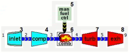
Figure 1.
Turbojet model in GSP. The digits in fine print are engine stations while the larger ones are GSP component numbers.
The degradation was simulated by changing the corresponding health parameters of the components, given by the efficiency and mass flow W of the compressor and the turbine. These parameters were chosen because they are affected by component faults, such as fouling and erosion. The corresponding degradation coefficients and were declared in GSP in percent and served as the map correction factors [47,50], i.e., they were used to calculate the degraded efficiency and mass flow from the reference values of and W, taken from the component maps:
The actual component degradation rate depends on aircraft missions and the environment in which it is operated. In civil aircraft, degradation is kept low (1–3%) to avoid increased fuel consumption, but it can grow to a higher number in the case of volcano ash encounters. In military helicopters operated in a desert environment, increased component degradation as high as 10% and short wing life are common. However, there are no reliable degradation data for micro turbojets. They are known for generally low efficiency and high manufacturing tolerance. In terms of component degradation, they are similar to small helicopter engines. In such high-speed systems, most of the physical faults have a higher impact than in a full-scale turbojet.
The assumed degradation levels of components were defined in the GSP Monte Carlo input controller. GSP implements a random generator with inverse normal distribution to calculate the input parameters for the simulation based on the given mean value and standard deviation [47]. Their values were selected to cover the possible variation of efficiency and flow. With the mean value equal and the standard deviation of 2%, the generated points well covered the three-sigma range, from to 0%. A multi-component degradation was simulated here because four degradation factors (two for the compressor and two for the turbine) were randomized at the same time. For these input data, GSP produced engine model outputs for defined degradation levels, appropriate for training neural networks. The expected variability of the chosen performance parameters needed a huge amount of simulated data to completely cover this multidimensional space by the AI regression model. It was practically impossible to obtain similar datasets from real flights.
2.2. Prediction of Component Degradation
In this study, component deterioration is considered for the single-stage radial compressor and axial turbine. Their deterioration is quantified by the difference between the actual component condition parameters and their baseline. From a thermodynamic perspective, the condition of gas path components is described by isentropic efficiency and mass flow W. Even if the degradation of the microturbine causes significant variation in component flow and efficiency, these parameters cannot be directly measured and so used to identify the engine health condition. However, some parameters measured by the sensors installed in the engine, such as temperature, pressure, rotational speed, etc., will be affected by component degradation and can be used for predicting the engine health status. Thus, these engine operating parameters are processed by ML models to solve the inverse problem of calculating the efficiency and mass flow of degraded components.
Figure 2 describes the methodology adopted in this work. The degradation prediction procedure includes the following steps:

Figure 2.
Methodology for component degradation prediction.
- The rig and flight data acquired from a real micro turbojet were used to validate the GSP model [45]. The validated model was subsequently used to simulate selected operating conditions to obtain the values of the virtual engine sensors, necessary to train and test the predictive techniques. The simulated parameters are listed in Table 2.
Table 2. Virtual sensors: simulated engine parameters.
- Three simulated flight regimes, (1) takeoff, (2) cruise and (3) air mission, were defined by different Mach (M) and altitude () values (Table 3). Additionally, M and were randomly distributed in flight regime 3. For each operating regime, the data generated by GSP embrace 500 operating points: 400 for training, and 100 for testing. Training and testing data were randomly selected from the same dataset.
Table 3. Ambient conditions and non-degraded component performance in simulated flight regimes.
- Both clean and degraded conditions of the compressor and the turbine were simulated. Two degraded performance parameters, i.e., efficiency and mass flow, were altered for two components: the compressor and turbine. Each of the four performance parameters was assigned random values to simulate the different levels of degradation severity using the GSP Monte Carlo input controller by selecting the mean value () and standard deviation (2%). In further analysis, the absolute values of efficiency and corrected flow were used instead of degradation factors in percent to avoid ambiguity.
- From the virtual sensors, four input vectors for training AI models were selected, as reported in Table 4. Input vector 1 consists of nine virtual sensors used for flight regimes 1 and 2, excluding speed and ambient conditions, which are constant. Input vector 2, used for flight regime 3, has a complete set of 12 parameters. Input vector 3, used for flight regimes 1 and 2, has only two parameters that correspond to the real sensors installed on the microturbine: and EGT. Input vector 4 used for flight regime 3 includes M, TT, PT, and EGT.
Table 4. Input vectors for ML models.
- The datasets generated by the GSP were used for training and testing ANN and ELM models to validate their accuracy in predicting the efficiency and mass flow W of both components. There were thus four outputs in each network, and the prediction models were able to find which component is degraded and to what extent. On this basis, the operator can classify engine health to a certain damage class.
- The comparison between ANN and ELM was performed on the same datasets, with input vectors 1 and 2. After that, the reduced input vectors 3 and 4 were used to verify the ELM prediction accuracy for all the degraded flight regimes.
2.3. Machine Learning Techniques
Due to their performance and versatility, machine learning methods are more and more widespread, for different purposes. In our earlier project, nonlinear autoregressive with exogenous inputs (NARX) neural networks (adequate for time-series data) were used to predict the exhaust gas temperature (EGT) with a one-step-ahead approach [51]. Results show a percentage error which almost always remains below 10% in absolute value. The EGT values were obtained by adopting another artificial intelligence technique, i.e., multigene genetic programming. NARX was also used to estimate specific fuel consumption during transient regimes [52]. More in detail, the developed system was composed of two different ANNs, the first one used to predict some engine parameters based on flight data and the second to predict the specific fuel consumption based on the parameters predicted from the first ANN and flight data. Results show good performance both in healthy and degraded conditions.
We also applied separately ANN and support vector (SVM)-based tools to the case of a single-spool turbojet for analyzing compressor and turbine degradation [32]. The results show very good performance, in particular, ANN gives better results in performance prediction, while SVM leads in engine health status prediction. Recently, we applied feed-forward neural networks (FFNNs) and kernel principal component analysis (KPCA) to estimate the degraded performance of the PW200 turboshaft [53].
Here, we focus on modeling JetCat turbojet performance and predicting its component degradation with AI-based regression algorithms, such as ANN and ELM. Unlike some other methods, only the current level of degradation is predicted, without taking into account past or future trends. This approach is well suited for micro turbojets, which have a short wing life and thus produce too little data to analyze their wear in a wider time perspective.
2.3.1. ANN-Based Regression
ANNs are machine learning-based tools that implement a virtual version of the human nervous system and its capacity to learn from experience. A typical ANN is formed by neurons, arranged in layers. Information fed in an ANN passes through the input layer, one or more hidden layers, to the output layer. Each neuron in a layer has its weight and is linked with the neurons of the adjacent layers. Input, hidden and output layers are formed by the input, hidden and output neurons, respectively. The number of input and output nodes is equal to the number of features given in input and to the number of variables to be predicted, respectively. The number of hidden layers and neurons is chosen arbitrarily, and it directly affects the ANN performance. Figure 3 reports a typical architecture of an ANN type used in this work.
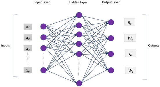
Figure 3.
Structure of ANN with one hidden layer.
Each neuron located in the hidden and output layers works by performing a weighted sum of the information received from the previous neurons and adding a bias. This process is described by the following equation:
where z represents the calculation result, is the weight of the link between the neuron in question and the i-th neuron from which it receives information, is the information received by the i-th neuron, n is the number of previous neurons that send information to the neuron in question, and b is the bias. The neuron output is finally subject to an activation function to normalize it. Weights and biases are computed in the training phase. During the training process, the ANN is informed with a series of example cases, including both the input features and the corresponding variables to be predicted. This serves to lead the ANN to calculate the proper weights and biases to obtain a small error between predictions and target values.
2.3.2. ELM-Based Regression
Extreme learning machine (ELM), introduced by Huang [34], is one of the most modern AI-based machine learning approaches. It has the single-layer feed-ahead neural network (SLFN) architecture in which the weights of hidden layers are randomly set, while the output ones are analytically determined via linear algebra operations. ELM was firstly implemented for the single hidden layer feed-forward neural networks and later extended to the generalized SLFNs, wherein the hidden layer no longer has to be neuron-like.
Unlike the traditional FFNN models, the hidden layer does not need to be tuned in ELM. The output characteristic of ELM for generalized SLFNs (for one output node case as an example) is
where x is the input vector, is the vector of the output weights in the hidden layer of L nodes, and is the hidden layer output mapping. virtually maps the records from the d-dimensional center area to the L-dimensional hidden-layer characteristic area , and thus, is certainly a characteristic mapping.
According to Bartlett’s theory, the smaller the norms of weights are, the higher generalization performance feedforward neural networks tend to have. We assume that this could be true for the generalized SLFNs in which the hidden layer is not neuron-like. Unlike conventional learning algorithms, ELM tends to attain not only the smallest training error, but also the smallest norm of output weights. We minimize and , where is the target output and is the hidden-layer output matrix:
The minimum norm least-square technique, as opposed to the traditional iterative optimization, is used in the implementation of ELM. The output weights can be obtained by the following formula:
in which is the Moore–Penrose generalized inverse of a matrix . Various techniques may be used to calculate the Moore–Penrose generalized inverse of a matrix, such as orthogonal projection, orthogonalization, iterative approach, or singular value decomposition (SVD). The orthogonal projection may be utilized if is nonsingular and , or is nonsingular and .
In this work, the implemented ELM model consists of three layers: the input layer (input vector 1/2/3), the hidden layers (neurons) and the output layer ( and , or and , Figure 4).

Figure 4.
Structure of the ELM network.
The ELM network was implemented in three steps:
- Randomly initialize the weights and thresholds of the ELM network and set the activation function.
- Calculate the hidden layer output matrix and its generalized inverse .
- Calculate the output vector.
3. Results
3.1. Engine Performance Simulations
The engine performance under different degradation conditions was simulated in GSP. Figure 5 shows the impact of compressor or turbine efficiency on the thrust (F) and the thrust specific fuel consumption (TSFC) both at sea level (flight regime 1) and cruise (flight regime 2) for different degradation levels. For only this figure, separate datasets for each component with the same distribution were generated to analyze the impact of single-component efficiency. In Figure 5a,c,e, compressor is degraded while the turbine is clean and vice versa in Figure 5b,d,e. The performance trend is the same for both components. An increase in efficiency leads to a rise in F and a decrease in TSFC. The variation of the microturbine performance due to the degradation of the components is similar at and sea level. The turbine efficiency has a slightly higher impact on TSFC than compressor efficiency.
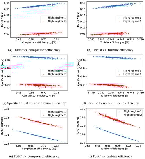
Figure 5.
Thrust and TSFC vs. compressor or turbine efficiency at sea level (flight regime 1) and cruise conditions (flight regime 2) for different degradation levels.
Figure 6 shows the distribution of altitude operating conditions, Mach number and component degradation factors in flight regime 3, generated by the GSP Monte Carlo component for training neural networks. The operating points are independent and stored in a random order, so they do not form a trend or time series. Figure 7 illustrates engine performance calculated by GSP for these random points. The values are scattered due to component degradation and variable flight conditions in flight regime 3.

Figure 6.
Flight regime 3: histograms of ambient temperature and pressure, airspeed and degradation factors, generated by the Monte Carlo method.

Figure 7.
Specific thrust vs. fuel flow for three flight regimes and varying degradation in both components.
3.2. ANN and ELM Predictions with Input Vectors 1 and 2
In this section, the predicted performance parameters of the two components is compared with the target virtual sensors data. The relative error is shown to evaluate the prediction accuracy.
Firstly, the condition at sea level was investigated for both compressor and turbine degradation (Flight regime 1). Figure 8 and Figure 9 show the results of ANN and ELM predictions for test data in the case of compressor and turbine degradation respectively. The target and predicted results are compared in subplots a and c, while the percentage prediction errors are presented in b and d. The curves for the target and predicted data overlay almost exactly. The error is very low (below 0.1%), so the target, which is plotted first, is usually covered completely by ELM and ANN data series.

Figure 8.
Compressor degradation in Flight regime 1 with Input vector 1: comparison between the target and prediction of the component performance parameters.

Figure 9.
Turbine degradation in flight regime 1 with input vector 1: comparison between the target and prediction of the component performance parameters.
Figure 10 and Figure 11 show the results of ANN and ELM predictions in flight regime 2 (, m), which is the cruise operating condition for the compressor and the turbine. Good prediction performance is still evident because both ANN and ELM show low percentage errors.

Figure 10.
Compressor degradation in flight regime 2 with input vector 1: comparison between the target and prediction of the component performance parameters.

Figure 11.
Turbine degradation in flight regime 2 with input vector 1: comparison between the target and prediction of the component performance parameters.
Finally, the last scenario analyzed with an extensive input vector (input vector 2) was the dataset with various Mach and altitude (flight regime 3). Figure 12 and Figure 13 show the results of ANN and ELM predictions. They are still remarkable, despite variable flight conditions.

Figure 12.
Compressor degradation in flight regime 3 with input vector 2: comparison between the target and prediction of the component performance parameters.

Figure 13.
Turbine degradation in flight regime 3 with input vector 2: comparison between the target and prediction of the component performance parameters.
3.3. ELM Prediction with a Reduced Number of Virtual Sensors (Input Vectors 3 and 4)
It is well known that feature selection, i.e., choosing input parameters, has a significant impact on the prediction accuracy of neural networks [53,54]. In this section, the prediction results obtained by ELM with a reduced dataset are reported. The chosen input variables correspond to the sensors that are installed on the real micro turbojet, i.e., exhaust gas temperature (EGT) and fuel flow rate. Fortunately, the performance deterioration of the aircraft engine mainly affects these two parameters, so they are strongly related to the efficiencies and flow capacities of the compressor and turbine.
Figure 14 and Figure 15 show the error in the prediction of the components’ performances under different flight regimes. Reducing the number of input variables decreases the accuracy of ELM in the case of many sensors. The error in the prediction of the mass flow for fixed Mach number (flight regimes 1 and 2) is negligible. The prediction is slightly worse for flight regime 3 with some peaks of error around 6% in the case of mass flow. These peaks are due to the unbalanced distribution of samples in the training set, given by the Monte Carlo, which can hinder the performance of ELM severely.

Figure 14.
ELM error of compressor degradation prediction with input vector 3 or 4.

Figure 15.
ELM error of turbine degradation prediction with input vector 3 or 4.
In ideal training sets, samples of different ranges of the target generally obey uniform distribution, but in Monte Carlo as well as in real flight data, the number of samples of some classes of target parameters may be several times higher than that of other classes. Consequently, ELM cannot effectively learn from minority classes and the trained network often predicts majority class samples more accurately than minorities. This is more critical than reducing the number of input variables.
The health of components can be classified by comparing the values of their performance parameters in healthy and degraded conditions. In our earlier publications [32,53], we introduced a component degradation class, ranging from 1 to 7, which combines reduced efficiency and mass flow in a single number. In this way, the prediction results will be used to classify component health and to make informed go/no-go decisions.
3.4. Overall Accuracy Metrics
The goodness of fit was evaluated in several ways to compare the results obtained from the sensitivity analysis and as a measure of the network’s prediction quality. In particular, the following metrics were used:
- Normalized root mean squared error (NRMSE);
- Coefficient of determination (CoD);
- Maximum relative absolute error (MaxRAE).
The NMSE is used to measure the average squared difference between the estimated values and the actual:
where
where represents the prediction of a parameter, is its actual value, s is the number of observations and std(y) is the standard deviation of the actual values. Normalizing the mean squared error facilitates the comparison between datasets or models with different scales. Normalization was done by the variance of .
Coefficient of determination (CoD) is a measure of the goodness of fit of a model and can reach one for the perfect fit:
Relative absolute error (RAE) can range from zero to one. The maximum RAE should be close to zero for a good model:
Table 5 shows that the implemented prediction methods give good results in all of the degradation scenarios, as confirmed by high CoD values. At each set of conditions, the prediction of the degradation level in the compressor and turbine has similar accuracy.
Table 5.
Metrics for input vectors 1 and 2 ELM and ANN.
Table 5 confirms that the use of extensive input variables leads to high prediction accuracy with slightly worse performance in the case of off-design conditions (flight regime 3). However, the use of few sensors in this flight regime reduces prediction performance significantly, with MaxRAE reaching 0.089 for turbine efficiency (Table 6).
Table 6.
ELM—metrics for reduced input vectors 3 and 4.
Finally, Table 7 reports the comparison of the training time for ANN and ELM for the three flight regimes and input Vectors 1 and 2, which is remarkably lower for ELM.
Table 7.
Mean training time (in arbitrary CPU units).
4. Discussion
The degradation of compressors and turbines is an inevitable process, so it is expected that this tool will help control the margin of acceptable degradation and plan appropriate maintenance actions. In previous generation diagnostic systems, engine operation was interrupted when arbitrary thresholds such as the EGT margin were exceeded by engine state variables. Currently, it is possible to predict non-measurable performance parameters of compressors and turbines, which enables deeper problem analysis and informed decision-making.
Many publications are limited to modeling only compressor degradation or predicting the overall performance of the engine without considering which component and to what extent has degraded. In our approach, both main components are worn to different levels and the same predictor can determine and distinguish their condition. Thanks to the proposed method, it is possible to determine which component has been degraded and to what extent. In this way, the method is ready for the various faults and wear scenarios that occur in the service. Often, from changes in efficiency and flow rate, it is possible to identify the mechanism or type of damage, e.g., erosion is accompanied by a reduction in efficiency and an increase in flow rate [7]. We have not prepared relevant data to demonstrate this but examples of damage classification can be found in other papers [55]. However, the randomization of parameters in line with the normal distribution allows the expected range of component parameter deviation to be evenly covered and thus the mapping of various degradation mechanisms observed in large and diverse populations of engines. This is another example of the successful application of the Monte Carlo method, commonly used in engine performance analysis [13,56].
In general, the degradation effects for large and small engines are similar, but microturbines have their unique features because some phenomena do not scale. In addition, the maps and degradation processes of radial compressors [57,58] differ from the axial ones that dominate in large engines. Most research on the degradation of microturbines is focused on power generation systems [59,60,61], such as Capstone C30, which have an operating time much longer than micro turbojets used in light aircraft and models. Although the engine layout is similar for air and ground systems, their designs differ significantly, e.g., with the type of bearings, the outlet nozzle, and lack of recuperation and generator. Moreover, the micro turbojets are devoid of any intake protection systems and so are more susceptible to damage from foreign objects than power-generation microturbines.
For the data generated for three flight regimes, we presented some major relationships between engine parameters and checked the impact of component efficiency changes on performance. It was a validation of the simulation rather than an attempt to analyze the degradation mechanisms of microturbines in depth. GSP and other tools offer ample opportunities to study the effects of efficiency and flow rate reduction on engine performance at various operating points, flight conditions, and mission profiles. This feature can help in solving operational problems or optimizing the mission of an aging engine fleet.
From the ML perspective, engine diagnostics can use classification or regression, which differ in details, e.g., the type of metrics used. In our prediction system, regression is performed, while most ELM applications in engines involve classification, so it is difficult to compare their results directly. Often, however, both approaches ultimately come down to classification, i.e., the decision to continue or suspend engine operations. It is similar in this case, where regression results are then used to assign the component to the proper health class.
Our observations are in line with other publications, e.g., Xu et. al showed that their ELM-based model had lower mean absolute error (MAE) and root-mean-square error (RMSE) and a shorter training time than other models based on other ANNs, i.e., BPNN, Elman, and LSTM [62]. In particular, their hybrid method based on ELM had RMSE equal to 0.32%, using the input vector with nine variables, while our ELM model has a maximum RMSE equal to 0.23% for the same vector length.
Our analysis dealt with simulated data, so under- or overfitting related to noise was not the case here. With the real data, to avoid these problems, preprocessing the data and implementing a more advanced version of ELM with regularization may be necessary. ELM is potentially more prone to overfitting but we obtained very similar errors in cross-validation when we used different sections of the dataset for training and testing. Additionally, our experiment with the complete and reduced input vector was designed to check if ELM has enough data to learn component degradation to avoid underfitting.
There are some limitations of ELM, which are directly related to the intrinsic features of the method. In some cases, using random weights can lead to an ill-conditioned matrix [63]. This was not observed here, but there are several new ELM variants without this drawback that achieve higher numerical stability and prediction accuracy than classical ELM. The choice of a specific ELM implementation depends on the application and the characteristics of the input data and typically requires testing. This work was limited to the classic ELM, as it worked stably and gave satisfactory accuracy. With this demonstration, one can judge what can be achieved with the basic ELM variant and whether to use this method instead of a traditional ANN, which is still a first-choice tool.
5. Conclusions
In this paper, ANN and ELM methods were applied to predict the efficiency and mass flow of the compressor and turbine, which are the main components of a micro turbojet. A digital twin of the real engine, already validated with experimental data from a test bench and real flights, gathered in the absence of degradation, was used. The validated model was subsequently extended to predict degraded engine performance. It was used to generate a dataset containing engine operating parameters for different degradation severity conditions with the Monte Carlo technique. A significant rise in the TSFC was observed when the component efficiency decreased. It was also found that component degradation in the micro turbojet had a similar impact in a high-altitude flight and at sea level.
The generated dataset was used to train the developed neural network with the ELM approach. Different lengths of the input vector were analyzed: an extensive one with a dozen of sensors and a reduced one with input variables corresponding to the real sensors installed on the engine. Furthermore, three different flight regimes were tested.
The use of ELM to estimate component degradation is an original contribution of this work. The analysis underlined that in the presence of many input variables, ELM has excellent prediction accuracy, comparable with ANN, but with a shorter CPU time. The reduced number of sensors gives remarkable predictions for mass flow but with slightly less accuracy (CoD about 80%) for component efficiency. Mean errors are generally acceptable but they reached 6% in some conditions in the case of off-design flight conditions, with variable Mach and altitude.
This study contributes to optimizing engine maintenance and ensuring necessary component performance, essential to completing the flight mission. Clearly, more research can be conducted in this area. Future work will base on the real flight data collected from several operated engines. Besides formal arrangements, this may require preprocessing the data and implementing a more advanced version of ELM with regularization. Undoubtedly, demonstrating an effective method for the in-service prediction of component degradation would expand the professional applications of micro turbojets.
Author Contributions
Conceptualization, M.G.D.G. and N.M.; methodology, N.M., M.G.D.G., A.M. and R.P.; software, N.M. and A.M.; validation, N.M., R.P. and M.G.D.G.; investigation, N.M., M.G.D.G., R.P. and A.M.; data curation, N.M.; writing—original draft preparation, N.M., M.G.D.G., A.M. and R.P.; writing—review and editing, R.P. and M.G.D.G.; visualization, N.M., A.M., R.P. and M.G.D.G.; supervision, M.G.D.G., A.F. and R.P.; project administration, A.F. All authors have read and agreed to the published version of the manuscript.
Funding
This research was funded by the Italian Ministry of University and Research, project PON “SMEA”, code PON03PE_00067_5.
Institutional Review Board Statement
Not applicable.
Informed Consent Statement
Not applicable.
Data Availability Statement
Data presented in this study are available on request from The University of Salento.
Conflicts of Interest
The authors declare no conflict of interest.
References
- Alozie, O.; Li, Y.G.; Diakostefanis, M.; Wu, X.; Shong, X.; Ren, W. Assessment of degradation equivalent operating time for aircraft gas turbine engines. Aeronaut. J. 2020, 124, 549–580. [Google Scholar] [CrossRef]
- Cruz-Manzo, S.; Panov, V.; Zhang, Y. Gas path fault and degradation modelling in twin-shaft gas turbines. Machines 2018, 6, 43. [Google Scholar] [CrossRef]
- Dvirnyk, Y.; Pavlenko, D.; Przysowa, R. Determination of Serviceability Limits of a Turboshaft Engine by the Criterion of Blade Natural Frequency and Stall Margin. Aerospace 2019, 6, 132. [Google Scholar] [CrossRef]
- Przybyła, B.S.; Przysowa, R.; Zapałowicz, Z. Implementation of a new inlet protection system into HEMS fleet. Aircr. Eng. Aerosp. Technol. 2020, 92, 67–79. [Google Scholar] [CrossRef]
- Walsh, P.P.; Fletcher, P. Gas Turbine Performance, 2nd ed.; Blackwell Science Ltd.: Oxford, UK, 2004. [Google Scholar]
- Fentaye, A.D.; Baheta, A.T.; Gilani, S.I.; Kyprianidis, K.G. A Review on Gas Turbine Gas-Path Diagnostics: State-of-the-art Methods, Challenges and Opportunities. Aerospace 2019, 6, 83. [Google Scholar] [CrossRef]
- Tahan, M.; Tsoutsanis, E.; Muhammad, M.; Abdul Karim, Z.A. Performance-based health monitoring, diagnostics and prognostics for condition-based maintenance of gas turbines: A review. Appl. Energy 2017, 198, 122–144. [Google Scholar] [CrossRef]
- Igie, U.; Diez-Gonzalez, P.; Giraud, A.; Minervino, O. Evaluating Gas Turbine Performance Using Machine-Generated Data: Quantifying Degradation and Impacts of Compressor Washing. J. Eng. Gas Turbines Power 2016, 138, 122601. [Google Scholar] [CrossRef]
- Sun, X.; Jafari, S.; Miran Fashandi, S.A.; Nikolaidis, T. Compressor Degradation Management Strategies for Gas Turbine Aero-Engine Controller Design. Energies 2021, 14, 5711. [Google Scholar] [CrossRef]
- Gou, L.; Liu, Z.; Fan, D.; Zheng, H. Aeroengine Robust Gain-Scheduling Control Based on Performance Degradation. IEEE Access 2020, 8, 104857–104869. [Google Scholar] [CrossRef]
- Zaccaria, V.; Ferrari, M.L.; Kyprianidis, K. Adaptive Control of Micro Gas Turbine for Engine Degradation Compensation. In Proceedings of the ASME Turbo Expo 2019: Turbomachinery Technical Conference and Exposition, Phoenix, AZ, USA, 17–21 June 2019. [Google Scholar] [CrossRef]
- De Giorgi, M.G.; Campilongo, S.; Ficarella, A. Predictions of operational degradation of the fan stage of an aircraft engine due to particulate ingestion. J. Eng. Gas Turbines Power 2015, 137, 052603. [Google Scholar] [CrossRef]
- Ellis, M.; Bojdo, N.; Filippone, A.; Clarkson, R. Monte carlo predictions of aero-engine performance degradation due to particle ingestion. Aerospace 2021, 8, 146. [Google Scholar] [CrossRef]
- Minijets. The Website for Fans of Light Jet Aircraft. Available online: https://minijets.org (accessed on 22 July 2022).
- Pavlenko, D.; Dvirnyk, Y.; Przysowa, R. Advanced Materials and Technologies for Compressor Blades of Small Turbofan Engines. Aerospace 2021, 8, 1. [Google Scholar] [CrossRef]
- Gaonkar, D.N.; Patel, R.N. Modeling and Simulation of Microturbine Based Distributed Generation System. In Proceedings of the 2006 IEEE Power India Conference, New Delhi, India, 10–12 April 2005; pp. 256–260. [Google Scholar]
- Badami, M.; Giovanni Ferrero, M.; Portoraro, A. Dynamic Parsimonious Model and Experimental Validation of a Gas Microturbine at Part-Load Conditions. Appl. Therm. Eng. 2015, 75, 14–23. [Google Scholar] [CrossRef]
- Alulema, V.; Valencia, E.; Cando, E.; Hidalgo, V.; Rodriguez, D. Propulsion Sizing Correlations for Electrical and Fuel Powered Unmanned Aerial Vehicles. Aerospace 2021, 8, 171. [Google Scholar] [CrossRef]
- Adamski, M. Analysis of Propulsion Systems of Unmanned Aerial Vehicles. J. Mar. Eng. Technol. 2018, 16, 291–297. [Google Scholar] [CrossRef]
- Oppong, F.; Spuy, S.J.V.D.; Diaby, A.L. An Overview on the Performance Investigation and Improvement of Micro Gas Turbine Engine. R&D J. S. Afr. Inst. Mech. Eng. 2015, 31, 35–41. [Google Scholar] [CrossRef]
- Capata, R.; Saracchini, M. Experimental Campaign Tests on Ultra Micro Gas Turbines, Fuel Supply Comparison and Optimization. Energies 2018, 11, 799. [Google Scholar] [CrossRef]
- Kim, M.J.; Kim, J.H.; Kim, T.S. The effects of internal leakage on the performance of a micro gas turbine. Appl. Energy 2018, 212, 175–184. [Google Scholar] [CrossRef]
- Talebi, S.; Tousi, A.; Madadi, A.; Kiaee, M. A methodology for identifying the most suitable measurements for engine level and component level gas path diagnostics of a micro gas turbine. Proc. Inst. Mech. Eng. Part C J. Mech. Eng. Sci. 2022, 236, 2646–2661. [Google Scholar] [CrossRef]
- Grannan, N.D.; Hoke, J.; McClearn, M.J.; Litke, P.; Schauer, F. Trends in jetCAT Microturbojet-Compressor Efficiency. In Proceedings of the AIAA SciTech Forum—55th AIAA Aerospace Sciences Meeting, Grapevine, TX, USA, 9–13 January 2017. [Google Scholar] [CrossRef]
- Thomas Jayachandran, A.V.; Omar, H.; Tkachenko, A.; Krishnakumar, A. Machine learning predictor for micro gas turbine performance evaluation. Aeronaut. Aerosp. Open Access J. 2020, 4, 172–180. [Google Scholar] [CrossRef]
- Gomes, E.E.B.; McCaffrey, D.; Garces, M.J.M.; Polizakis, A.L.; Pilidis, P. Comparative Analysis of Microturbines Performance Deterioration and Diagnostics. In Proceedings of the ASME Turbo Expo 2006: Power for Land, Sea, and Air, Barcelona, Spain, 8–11 May 2006; pp. 269–276. [Google Scholar] [CrossRef]
- Rahman, M.; Zaccaria, V.; Zhao, X.; Kyprianidis, K. Diagnostics-Oriented Modelling of Micro Gas Turbines for Fleet Monitoring and Maintenance Optimization. Processes 2018, 6, 216. [Google Scholar] [CrossRef]
- Khustochka, O.; Chernysh, S.; Yepifanov, S.; Ugryumov, M.; Przysowa, R. Estimation of Performance Parameters of Turbine Engine Components Using Experimental Data in Parametric Uncertainty Conditions. Aerospace 2020, 7, 6. [Google Scholar] [CrossRef]
- Hanachi, H.; Mechefske, C.; Liu, J.; Banerjee, A.; Chen, Y. Performance-based gas turbine health monitoring, diagnostics, and prognostics: A survey. IEEE Trans. Reliab. 2018, 67, 1340–1363. [Google Scholar] [CrossRef]
- de Castro-Cros, M.; Velasco, M.; Angulo, C. Machine-Learning-Based Condition Assessment of Gas Turbines—A Review. Energies 2021, 14, 8468. [Google Scholar] [CrossRef]
- Akpudo, U.E.; Hur, J.W. Investigating the Efficiencies of Fusion Algorithms for Accurate Equipment Monitoring and Prognostics. Energies 2022, 15, 2204. [Google Scholar] [CrossRef]
- De Giorgi, M.G.; Campilongo, S.; Ficarella, A. A Diagnostics Tool for Aero-Engines Health Monitoring Using Machine Learning Technique. Energy Procedia 2018, 148, 860–867. [Google Scholar] [CrossRef]
- De Giorgi, M.G.; Campilongo, S.; Ficarella, A. Development of a Real Time Intelligent Health Monitoring Platform for Aero-Engine. MATEC Web Conf. 2018, 233, 00007. [Google Scholar] [CrossRef]
- Huang, G.B.; Zhu, Q.Y.; Siew, C.K. Extreme learning machine: Theory and applications. Neurocomputing 2006, 70, 489–501. [Google Scholar] [CrossRef]
- Albadr, M.A.A.; Tiun, S. Extreme Learning Machine: A Review. Int. J. Appl. Eng. Res. 2017, 12, 4610–4623. [Google Scholar]
- Zhao, Y.P.; Huang, G.; Hu, Q.K.; Tan, J.F.; Wang, J.J.; Yang, Z. Soft Extreme Learning Machine for Fault Detection of Aircraft Engine. Aerosp. Sci. Technol. 2019, 91, 70–81. [Google Scholar] [CrossRef]
- Lu, F.; Jiang, C.; Huang, J.; Wang, Y.; You, C. A Novel Data Hierarchical Fusion Method for Gas Turbine Engine Performance Fault Diagnosis. Energies 2016, 9, 828. [Google Scholar] [CrossRef]
- Jiang, W.; Xu, Y.; Shan, Y.; Liu, H. Degradation Tendency Measurement of Aircraft Engines Based on FEEMD Permutation Entropy and Regularized Extreme Learning Machine Using Multi-Sensor Data. Energies 2018, 11, 3301. [Google Scholar] [CrossRef]
- Pérez-Ruiz, J.L.; Tang, Y.; Loboda, I. Aircraft Engine Gas-Path Monitoring and Diagnostics Framework Based on a Hybrid Fault Recognition Approach. Aerospace 2021, 8, 232. [Google Scholar] [CrossRef]
- Liu, X.; Liu, L.; Wang, L.; Guo, Q.; Peng, X. Performance Sensing Data Prediction for an Aircraft Auxiliary Power Unit Using the Optimized Extreme Learning Machine. Sensors 2019, 19, 3935. [Google Scholar] [CrossRef]
- Bai, M.; Liu, J.; Ma, Y.; Zhao, X.; Long, Z.; Yu, D. Long Short-Term Memory Network-Based Normal Pattern Group for Fault Detection of Three-Shaft Marine Gas Turbine. Energies 2020, 14, 13. [Google Scholar] [CrossRef]
- Berghout, T.; Mouss, L.H.; Kadri, O.; Saïdi, L.; Benbouzid, M. Aircraft Engines Remaining Useful Life Prediction with an Improved Online Sequential Extreme Learning Machine. Appl. Sci. 2020, 10, 1062. [Google Scholar] [CrossRef]
- Chen, H.; Li, Q.; Pang, S.; Zhou, W. A State Space Modeling Method for Aero-Engine Based on AFOS-ELM. Energies 2022, 15, 3903. [Google Scholar] [CrossRef]
- Gu, Z.; Pang, S.; Zhou, W.; Li, Y.; Li, Q. An Online Data-Driven LPV Modeling Method for Turbo-Shaft Engines. Energies 2022, 15, 1255. [Google Scholar] [CrossRef]
- Erario, M.L.; De Giorgi, M.G.; Przysowa, R. Model-Based Dynamic Performance Simulation of a Microturbine Using Flight Test Data. Aerospace 2022, 9, 60. [Google Scholar] [CrossRef]
- Visser, W.P.J.; Broomhead, M.J. GSP, a Generic Object-Oriented Gas Turbine Simulation Environment. In Proceedings of the ASME Turbo Expo 2000: Power for Land, Sea, and Air, Munich, Germany, 8–11 May 2000. [Google Scholar] [CrossRef]
- GSP Development Team GSP 11 User Manual; NLR—Royal Netherlands Aerospace Centre: Amsterdam, The Netherlands, 2021.
- JetCatRX Turbines with V10 ECU; Ingenieur-Büro CAT, M. Zipperer GmbH: Staufen, Germany, 2010; pp. 1–54.
- Hajduk, J.; Rykaczewski, D. Possibilities of Developing Aerial Target System JET-2 (Możliwości Rozwoju Zestawu Odrzutowych Celów Powietrznych Zocp-Jet2). In Mechanika w Lotnictwie ML-XVIII Tom 2 (Mechanics in Aviation ML-XVIII Volume 2); Sibilski, K., Ed.; PTMTS: Warszawa, Poland, 2018; pp. 139–154. [Google Scholar]
- Visser, W.P.J.; Broomhead, M.J.; Kogenhop, O.; Rademaker, E.R. Technical Manual of Gas Turbine Simulation Program; Technical Report NLR-TR-2010-343-Issue-2; National Aerospace Laboratory NLR: Amsterdam, The Nederlands, 2010. [Google Scholar]
- De Giorgi, M.G.; Quarta, M. Hybrid MultiGene Genetic Programming—Artificial Neural Networks Approach for Dynamic Performance Prediction of an Aeroengine. Aerosp. Sci. Technol. 2020, 103, 105902. [Google Scholar] [CrossRef]
- De Giorgi, M.G.; Strafella, L.; Ficarella, A. Neural nonlinear autoregressive model with exogenous input (Narx) for turboshaft aeroengine fuel control unit model. Aerospace 2021, 8, 206. [Google Scholar] [CrossRef]
- De Giorgi, M.G.; Strafella, L.; Menga, N.; Ficarella, A. Intelligent Combined Neural Network and Kernel Principal Component Analysis Tool for Engine Health Monitoring Purposes. Aerospace 2022, 9, 118. [Google Scholar] [CrossRef]
- Khumprom, P.; Grewell, D.; Yodo, N. Deep Neural Network Feature Selection Approaches for Data-Driven Prognostic Model of Aircraft Engines. Aerospace 2020, 7, 132. [Google Scholar] [CrossRef]
- Yoon, J.E.; Lee, J.J.; Kim, T.S.; Sohn, J.L. Analysis of performance deterioration of a micro gas turbine and the use of neural network for predicting deteriorated component characteristics. J. Mech. Sci. Technol. 2008, 22, 2516–2525. [Google Scholar] [CrossRef]
- Kurzke, J.; Halliwell, I. Monte Carlo Simulations. In Propulsion and Power: An Exploration of Gas Turbine Performance Modeling; Springer International Publishing: Cham, Switzerland, 2018; pp. 439–575. [Google Scholar] [CrossRef]
- Son, S.; Cho, S.K.; Lee, J.I. Experimental investigation on performance degradation of a supercritical CO2 radial compressor by foreign object damage. Appl. Therm. Eng. 2021, 183, 116229. [Google Scholar] [CrossRef]
- Safiyullah, F.; Sulaiman, S.; Naz, M.; Jasmani, M.; Ghazali, S. Prediction on performance degradation and maintenance of centrifugal gas compressors using genetic programming. Energy 2018, 158, 485–494. [Google Scholar] [CrossRef]
- Davison, C.R.; Birk, A.M. Automated Fault Diagnosis of a Micro Turbine With Comparison to a Neural Network Technique. In Proceedings of the ASME Turbo Expo 2006: Power for Land, Sea, and Air, Barcelona, Spain, 8–11 May 2006; pp. 795–804. [Google Scholar] [CrossRef]
- Liu, Y.; Banerjee, A.; Ravichandran, T.; Kumar, A.; Heppler, G. Data analytics for performance monitoring of gas turbine engine. In Proceedings of the Annual Conference of the Prognostics and Health Management Society, Philadelphia, PA, USA, 24–27 September 2018; pp. 201–203. [Google Scholar] [CrossRef]
- Olsson, T.; Ramentol, E.; Rahman, M.; Oostveen, M.; Kyprianidis, K. A data-driven approach for predicting long-term degradation of a fleet of micro gas turbines. Energy AI 2021, 4, 100064. [Google Scholar] [CrossRef]
- Xu, M.; Wang, J.; Liu, J.; Li, M.; Geng, J.; Wu, Y.; Song, Z. An Improved Hybrid Modeling Method Based on Extreme Learning Machine for Gas Turbine Engine. Aerosp. Sci. Technol. 2020, 107, 106333. [Google Scholar] [CrossRef]
- Yang, X.; Pang, S.; Shen, W.; Lin, X.; Jiang, K.; Wang, Y. Aero Engine Fault Diagnosis Using an Optimized Extreme Learning Machine. Int. J. Aerosp. Eng. 2016, 2016, 7892875. [Google Scholar] [CrossRef]


Publisher’s Note: MDPI stays neutral with regard to jurisdictional claims in published maps and institutional affiliations. |
© 2022 by the authors. Licensee MDPI, Basel, Switzerland. This article is an open access article distributed under the terms and conditions of the Creative Commons Attribution (CC BY) license (https://creativecommons.org/licenses/by/4.0/).