Continuous Adjoint Topology Optimization of Duct Flow Configurations with Explicit Volume Constraint for Design Variable Update

Abstract

The adjoint method is a very promising gradient-based optimisation framework for computational fluid dynamics (CFD), because of its independence of the computation cost from the number of design variables. With the aim of improving the robustness of the continuous adjoint topology optimization, this paper presents a direct method for the design variable update. Based on the intrinsic feature of the topology optimization, this straightforward update method explicitly controls the design variable target volume, precluding any case-dependent parameters. The details of its implementation are discussed with regard to an existing open-source continuous adjoint topology optimization solver. The performance of this alternative method is tested on complex 3D engineering problems with duct configuration, and no impact on the computational demands or numerical stability has been observed in the simulations.

1. Introduction

The numerical optimization methods for computational fluid dynamics (CFD) find their use in various branches of engineering, because they can contribute to the improvement of a fluid flow system performance through relatively easy design interventions. With the focus on the numerical stability of the optimization simulations, the present work is restricted to the gradient-based topology optimization for steady-state isothermal incompressible flows of a Newtonian fluid. The case under consideration is an example of a constrained optimization problem, in which the constraints are given by a set of partial differential equations that govern the fluid flow (e.g., the velocity and pressure equations in the case of a laminar flow). Unlike in the classical gradient-based optimization approaches, in which the computational cost scales linearly with the number of design variables, the adjoint optimization method has highly desirable feature that its computational cost does not depend directly on the size of the design variable space [1]. For the continuous adjoint optimization framework, the set of adjoint equations is derived from their primal counterparts, with the aim of providing the objective function sensitivity independent of the derivatives of the flow variables w.r.t. the design variable. With this obtained sensitivity, the design variable is updated toward the minimization of the specified objective function. Hence, the optimization computation cost is related to the effort of solving the augmented set of equations, and not directly dependent on the design variable space size [2]. The price to be paid for this beneficial method property is the increased model complexity, which is then mirrored in the numerical stability.

The advantages of the adjoint-based optimisation in the computational engineering have long been recognised (most notably in structural mechanics), with the majority of the early work performed focusing on the needs of the aeronautical industry [3]. The uptake of the CFD adjoint optimization came with the improvements in the numerical modelling, when the adjoint optimization method was extended to capture more complex physical phenomena, ranging from the turbulence modelling [4] to the conjugate heat transfer [5]. As a part of these developments, the complexity of the method was tackled through a careful implementation of the grid sensitivity [6], turbulence modeling near-wall treatment [7], or fluid–solid interface [8], just to name a few aspects. At present, the adjoint method is successfully used for the shape optimization, in which the surface sensitivities are used to calculate the modification of the boundaries of the investigated body. This is shown, among other areas, in the aerodynamic applications [9], and in particular for the car aerodynamics [10]. Another way to make use of the adjoint method is the topology optimization, in which the volume sensitivities are used to distinguish between the important and counterproductive areas within the numerical domain, whereas boundaries of the investigated body remain unchanged. This approach is presented, e.g., for the intake port optimization [11], or the exhaust system case [12].

In CFD topology optimization, the design variable is the penalty function, for which all cells within the domain are examined individually; if a cell does not contribute to the minimization of the specified objective function, it is penalized by introducing the Darcy porosity (hence, the flow is blocked in that cell), and the procedure of the design variable update continues until the optimization criterion is met [13]. A very simple update approach, yet very illustrative of the gradient-based optimization is the steepest gradient descent. In this approach, the design variable is updated by a portion of the calculated sensitivity, iterating through a number of updated steps [14]. The problem arises with defining the step size, because the sensitivity can take arbitrary values (depending on the flow characteristics, it can vary by several orders of magnitude). If the selected gradient descent step size is either too small or too big, the optimization process can be prohibitively long or fail in the objective function minimisation. Available in the literature are better-designed and more advanced update methods that do not suffer from these problems, such as the quasi-Newton method or method of moving asymptotes [15], but they all follow the same basic idea (thus inheriting related problems) which is that a suitable value of the design variable is sought. Instead, the explicit scheme for the design variable update proposed here makes use of the basic idea in the topology optimization that the counterproductive cells within the domain are either to be blocked or left free (based on the calculated sensitivity); hence, the design variable value is adjusted between zero and unity. The aim is in this way to derive the scheme which will ensure numerically robust optimization simulations, while satisfying directly the volume constraint without additional computational overload.

As the developments presented in this paper are making use of the work already to be found in the literature, Section 2 summarises the theoretical background in a condensed manner. The novel aspect in this paper is to present the explicit updating idea and its implementation, and this is given in Section 3. Finally, the performance of this novel method is shown in Section 4 for a complex engineering fluid flow problem with duct configuration, and the concluding remarks are given in Section 5.

2. Theoretical Background

The topology optimization for a fluid flow problem can be formulated as the minimization of the selected objective function J, subject to the fluid flow constraints. For the steady-state case of incompressible isothermal turbulent flow of Newtonian fluid, these constraints represent the governing equations, Navier–Stokes (with Darcy term) and continuity, written in the residual form

$$\begin{array}{c}\hfill R^{\mathbf{v}}=(\mathbf{v}·\nabla )\mathbf{v}+\nabla p-\nabla ·\left(2{\nu }_{eff}D\left(\mathbf{v}\right)\right)+\alpha d_{\alpha }\mathbf{v}=0,\\ \hfill R^p=-\nabla ·\mathbf{v}=0,\end{array}$$

(1)

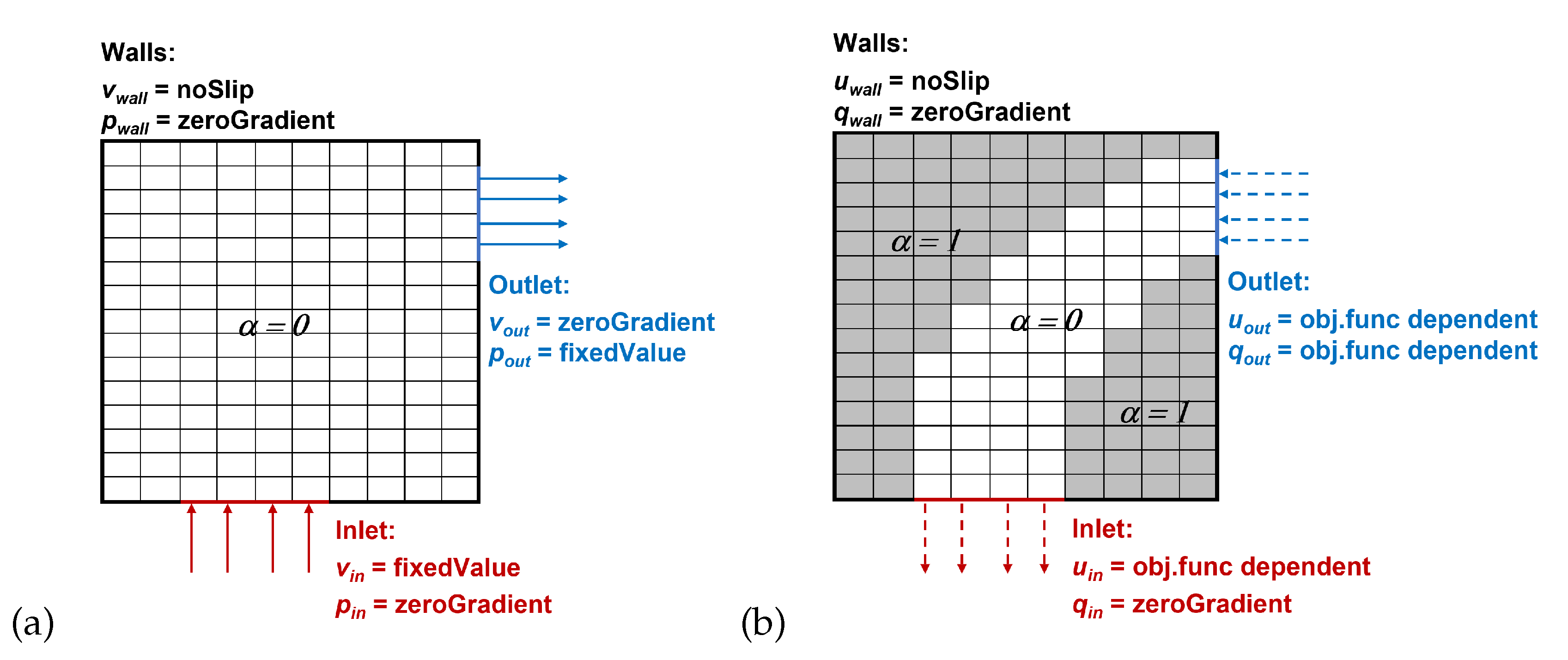
where $\mathbf{v}$ and p are the primal velocity vector and primal kinematic pressure, respectively, ${\nu }_{eff}=\nu +{\nu }_t$ is the effective kinematic viscosity comprising the laminar and turbulent part (obtained from the appropriate turbulence model, which is additionally to be solved), and $D\left(\mathbf{v}\right)=\frac{1}{2}(\nabla \mathbf{v}+{(\nabla \mathbf{v})}^T)$ is the primal rate of strain tensor. The above set of equations is complemented by the corresponding boundary conditions—at the inlet Dirichlet for velocity and Neumann for pressure, at the outlet Dirichlet for pressure (typically zero) and Neumann for velocity, and no slip at wall surfaces (Figure 1a).

The central element of topology optimization is the Darcy porosity term in the momentum equation, through which the design variable $\alpha$ is introduced and scaled with the Darcy porosity coefficient $d_{\alpha }$. The role of $\alpha$ is to mark those cells that need to be penalized (indicated with shadow in Figure 1b), based on whether or not an individual cell contributes to minimizing the objective function. The value for the porosity coefficient can be calculated from the Darcy number estimation [16]

$$\begin{array}{c}\hfill Da=\frac{\nu }{d_{\alpha }{\ell }^2}={10}^{-5},\end{array}$$

(2)

where $Da$ quantifies the ratio between the viscous and porous forces, $\nu$ is the kinematic viscosity, and ℓ is the characteristic length (e.g., the inlet hydraulic diameter).

The work presented in this paper has been performed using adjointShapeOptimizationFoam, the continuous adjoint topology optimization solver (despite what the name suggests) provided in the open-source CFD suite OpenFOAM^® version 1906 [17,18]. Acknowledging its limitations and restrictions, this solver has been selected for its accessible structure which allows for a transparent implementation of the presented method. The solver is developed from the simpleFoam (standard steady-state solver for incompressible isothermal turbulent flow of Newtonian fluids) by deploying the frozen turbulence assumption in the adjoint equations, adopting the duct flow configuration (the boundaries comprising the inlet, outlet, and wall surfaces $\mathsf{\Gamma }={\mathsf{\Gamma }}_{inlet}\cup {\mathsf{\Gamma }}_{outlet}\cup {\mathsf{\Gamma }}_{walls}$, according to the sketch in Figure 1a), and taking the total pressure loss between the inlet and outlet as the objective function to be minimized:

$$\begin{array}{c}\hfill J=J_{\mathsf{\Omega }}+J_{\mathsf{\Gamma }}=-{\int }_{{\mathsf{\Gamma }}_{inlet}+{\mathsf{\Gamma }}_{outlet}}d\mathsf{\Gamma }(p+v^2/2)\mathbf{v}·\mathbf{n},\end{array}$$

(3)

where v is the velocity magnitude (at inlet and outlet, respectively), and it is assumed that no contribution to the objective function from the domain interior $\mathsf{\Omega }$ is present ($J_{\mathsf{\Omega }}=0$).

This constraint flow optimization problem can be solved by looking at the augmented objective function $L=J+{\int }_{\mathsf{\Omega }}{R}^{x_i}{y}_{i}d\mathsf{\Omega }$, in which the Lagrange multipliers $y_i$ are introduced adjoint to their respective primal flow governing equations $R^{x_i}$. The aim is to construct these adjoints such that the objective function gradient dependency on the derivatives of the flow variables w.r.t. the design variables is canceled. After an extensive mathematical manipulation, the final set of adjoint equations is obtained as

$$\begin{array}{c}\hfill R^{\mathbf{u}}=-(\mathbf{v}·\nabla )\mathbf{u}-\nabla \mathbf{u}·\mathbf{v}+\nabla q-\nabla ·\left(2{\nu }_{eff}D\left(\mathbf{u}\right)\right)+\alpha d_{\alpha }\mathbf{u}=0,\\ \hfill R^q=\nabla ·\mathbf{u}=0,\end{array}$$

(4)

where $\mathbf{u}$ is the adjoint velocity vector, q is the adjoint pressure, and $D\left(\mathbf{u}\right)$ is the adjoint rate of strain tensor. Taking the total pressure loss as the objective function to be minimized for the duct flow configuration, as defined by Equation (3), the adjoint boundary conditions are defined for different boundary sections

$$\begin{array}{ccc}\hfill \mathrm{inlet}\mathrm{and}\mathrm{walls}:& \hfill & \hfill \mathrm{outlet}:\\ \hfill u_t=0,& \hfill & \hfill q=\mathbf{u}·\mathbf{v}+u_n{v}_n+{\nu }_{eff}(\mathbf{n}·\nabla )u_n-(p+v^2/2)-v_n^2,\\ \hfill u_n=\left\{\begin{array}{cc}0\hfill & \mathrm{wall},\hfill \\ -v_n\hfill & \mathrm{inlet},\hfill \end{array}\right.& \hfill & \hfill 0=v_n(u_t-v_t)+{\nu }_{eff}(\mathbf{n}·\nabla )u_t,\end{array}$$

(5)

where the vectors are decomposed into their normal and tangential components (with respect to the boundary surface normal unit vector $\mathbf{n}$ and its perpendicular tangential unit vector $\mathbf{t}\perp \mathbf{n}$), the primal velocity $\mathbf{v}=v_t\mathbf{t}+v_n\mathbf{n}$ and the adjoint velocity $\mathbf{u}=u_t\mathbf{t}+u_n\mathbf{n}$, the zero-gradient boundary condition is imposed for the adjoint pressure at the inlet and walls (analogous to its primal counterpart), and the normal component of the adjoint velocity at the outlet is obtained from the continuity requirement (Figure 1b).

Although the form of the adjoint equations corresponds to that of the primal equations (including the Darcy term in the adjoint velocity equation, which accommodates the design variable), one needs to note two main differences between the equation sets (1) and (4): in the adjoint velocity equation the convection term has a negative sign (therefore, in Figure 1 the vectors for (a) and (b) have opposite signs), and there is an additional transpose convection term which is not conservative and thus can cause numerical problems.

A more elaborate explanation of the continuous adjoint topology optimization method, as well as the full derivation of the adjoint equations and related boundary conditions can be found elsewhere [19,20]. In the present section, however, the complete set of equations is given just to describe the optimization workflow. Namely, in order to minimize the objective function, Equation (3), one needs to solve the equation sets (1) and (4), complemented by appropriate boundary conditions (standard set for the primal equations, and the equation set (5) for the adjoint equations). Having solved the presented set of equations, the topology sensitivity is obtained from the calculated primal and adjoint fields:

$$\begin{array}{c}\hfill \frac{\partial L}{\partial \alpha }=sens=\mathbf{u}·\mathbf{v},\end{array}$$

(6)

and the design variable $\alpha$ is updated by using the calculated sensitivity, e.g., through the steepest descent method:

$$\begin{array}{c}\hfill {\alpha }^{new}={\alpha }^{old}(1-\gamma )+\left[min(max({\alpha }^{old}-\lambda sens,0),1)\right]\gamma ,\end{array}$$

(7)

where $\lambda$ is the gradient descent step, incorporating the porosity coefficient from Equation (2). To improve the stability of the design variable update, the under-relaxation factor $\gamma$ can be applied, and the bounding within the physical limits needs to be imposed.

An exemplary idea behind the gradient-based optimisation is illustrated in Figure 2, where the gradient of the objective function from Equation (6) drives the update of the design variable from the initial value ${\alpha }_0$ to the optimal one ${\alpha }_1$. This process goes through a number of steps with size $\lambda$, and if $\lambda$ is too big, the update can jump to the opposite branch of the design variable curve (in Figure 2 indicated with gray dotted curves).

3. Explicit Volume Constraint Update

The centrepiece of the continuous adjoint optimization is to advance the design variables update based on the calculated sensitivity. It is very often required in the topology optimization that the percentage of the computational domain occupied by $\alpha$ be limited (e.g., due to the geometrical limitations, structural requirements, or economical considerations). This volume constraint can be implemented into the design variable update through the method of moving asymptotes [21].

In the alternative approach, however, one starts from the intrinsic feature of the topology optimization that $\alpha$ takes the value of unity if the calculated sensitivity indicates that the cell is counterproductive for minimising the selected objective function. Under this condition, the considered cell is to be blocked (the porosity is introduced); otherwise, the cell is left free ($\alpha$ takes the zero value). Mathematically, this behavior can be described with the sigmoid function, which changes from 0 to 1 as the independent variable x switches sides of appropriately selected limiting value $x_L$: $\alpha =1-1/[exp(C_1(x-x_L)+C_2)+1]$. Here, the coefficient $C_1$ defines the slope and $C_2$ positions the inflection point of the sigmoid function around the limiting value $x_L$. In the present case, the independent variable represents the sensitivity, which can take any value depending on the flow conditions, Equation (6). One can introduce the coefficient modification $C_2=C_1(x_L-C_0)$, and through a conveniently selected $C_0$ value, position the sigmoid function around the desired value for any $x_L$:

$$\begin{array}{c}\hfill \alpha =1-\frac{1}{e^{C_1(x-C_0)}+1},\end{array}$$

(8)

where the graphical representation in Figure 3 illustrates how the slope and inflection point are guided with $C_1$ and $C_0$, respectively.

With the notion that the coefficient selection can control the mapping between the calculated sensitivity and the design variable distribution, it is left to define the framework for calculating the needed coefficients. As $C_1$ is increased, the range of x for which the resulting $\alpha$ will be between 0 and 1 gets smaller. This grey zone is unwanted in the topology optimization, because the cell is either to be blocked or left free. By letting $C_1$ grow suitably high, Equation (8) tends towards the step function (as indicated in Figure 3 with the color sequence red–green–blue–black), which eliminates the grey zone. On the other hand, taking the high $C_1$ limit into the introduced coefficient modification yields $C_0$ to tend toward $x_L$. Within OpenFOAM^® the step function is available as $pos\left(s\right)$, which evaluates to 1 if the scalar expression s yields a non-negative value, or 0 otherwise [17]. Finally, by suitably selecting the coefficients of the sigmoid function, it can be turned into the step function $pos\left(s\right)=pos(x-x_L)$ to mark for blocking the part of the domain where the calculated sensitivity is greater than the limiting sensitivity value.

It is drawn in Figure 4 how the limiting sensitivity value can be sought, such that the volume constraint (i.e., the blocking cells’ volume does not exceed the pre-defined target value) is satisfied explicitly. Given that the calculated sensitivities can span several orders of magnitude, the procedure consists of $n_{loops}$ steps through the logarithmic scale. It starts by setting the sensitivity threshold at the highest obtained sensitivity value $sen{s}_{max}$ (in order to start with the smallest portion of the domain marked for blocking), subsequently reducing it toward the lowest sensitivity value $sen{s}_{min}$ (at which the entire domain with positive sensitivity is marked for blocking). This threshold reduction is performed with the step size that covers equally all range decades, and at every step the obtained blocking volume is recalculated in order to stop the process when the target volume is reached:

$$\begin{array}{c}\hfill x_L=\mathrm{range}\left[log\left(sen{s}_{max}\right),log\left(sen{s}_{min}\right),n_{loops}\right],\\ \hfill sen{s}_L={10}^{x_L},\\ \hfill \alpha =pos(sens-sen{s}_L),\\ \hfill vol={\int }_{\mathsf{\Omega }}\alpha dV\le vo{t}_T,\end{array}$$

(9)

where $sen{s}_L$ is the limiting sensitivity, as calculated with $n_{loops}$ steps, for which the target volume of the blocking cells $vo{l}_T$ is reached.

The implementation of the explicit design variable update into an existing continuous adjoint optimization solver boils down to introducing the procedure summarized in Equation (9) instead of the existing design variable update (e.g., Equation (7) for the steepest gradient descent expression). In further work, the step function $pos\left(s\right)$ replaced the continuous distribution defined by Equation (8). The search for $sen{s}_L$ is further simplified if the calculated sensitivity field is normalised with the maximum obtained value $sen{s}_{max}$, so that the loop is performed over the decades (${10}^0,{10}^{-1},{10}^{-2},\cdots ,{10}^{-m}$ in Figure 4). Empirically, one can set the maximum number of search decades m (estimating that the blocking cells are found within m orders of magnitude of $sen{s}_{max}$) and select the number of divisions per decade p (assuming that each decade is split in p-th), to estimate the number of search steps $n_{loops}=mp$. To complete the flowchart of the continuous adjoint topology optimisation with the design variable update fulfilling explicitly the volume constraint, it is indicated in Figure 5 that with the design variable update completed, the design cycles can be repeated for $n_{cycles}$ times, in order to adjust to the latest distribution of $\alpha$.

4. Topology Optimization Results

The presented topology optimization framework is applied to a 3D flow distribution duct (Figure 6), in which the air flow is entering below through a central pipe (inlet diameter $d_{in}$ = 4 cm) and needs to be brought above on two sides to leave through the slits (opening thickness $t_{out}$ = 5 mm) incurring the lowest possible total pressure loss (Equation (3)). The related geometry, with the overall dimensions $20\times 20\times$ 20 cm, is shown in Figure 6a. Colored in green is the inlet with $v_{in}$ = 8 m/s fixed inlet velocity. The outlet is colored violet, and the walls are cyan. From the steady-state solution of non-optimized case, shown in Figure 6b, the characteristic flow pattern can be inquired (from the streamlines and velocity vectors and contourplots). The jet flow is entering from the pipe and hitting the opposite wall of the housing; subsequently, it splits and bends in the horizontal plane, creating an adjacent recirculation zone. Further downstream, it bends in the vertical plane and leaves through the upper slits.

In these simulations, the effects of turbulence were modelled by using the $k-\epsilon$ model [22]. The porosity coefficient in this case was defined by using Equation (2), and the number of search loops in Equation (9) was set to $n_{loops}=12$. In order to scrutinize the optimization requirement to limit the volume occupied by the cells marked for blocking, the simulations with varying $vo{l}_T$ were performed. Starting with $vo{l}_T=10\%$ as the expected relative target volume, the regions that contribute the most to the minimization of the total pressure loss are marked for blocking (Figure 7a) immediately after the pipe enters the duct, as well as the the corners between the horizontal and vertical duct section. When this parameter is increased to $vo{l}_T=20\%$, these dead regions are highlighted more (Figure 7b), and extended to the recirculation zone in the horizontal duct section. Increasing this parameter even further $vo{l}_T=30\%$, the blocking region forges ahead into the vertical duct section (Figure 7c). The solution obtained as the topology optimization outcome can be understood as the channeling of the jet flow coming from the inlet pipe, bending it sideways at the back wall of the duct, and finally after bending upward, streamlining the expansion of the flow from the back wall toward the outlet slits.

Looking at the variation of the objective function (relative to the initial objective function value, calculated from the converged solution of non-optimized case) throughout the design cycles $n_{cycles}$, Figure 8 shows that most of the objective function reduction is reached within the first three design cycles, and after the fourth cycle, further reduction becomes negligible. On the other hand, by increasing the limit for the allowed occupied volume (relative to the total volume of the domain), better streamlining of the flow can be achieved, which is reflected in stronger reduction of the objective function (in Figure 8 the values from the last design cycle). With $vo{t}_T=10\%$ (Figure 7a), the flow is penalized mostly in the duct corners, which brings $3.5\%$ reduction of J. For $vo{t}_T=20\%$ (Figure 7b), the jet flow is also channeled through the central duct section, and J is reduced by $5.5\%$. A smooth transition further into the vertical duct section is featured with $vo{t}_T=30\%$ (Figure 7c), which yields $6\%$ improvement of J. It needs to be noted, however, that the rate at which the objective function is reduced becomes lower as $vo{t}_T$ moves to higher values, which is a clear indication that $vo{t}_T$ is not to be arbitrarily varied.

For comparison of the performance, the same topology optimization was repeated by using the steepest gradient descent method (Equation (7)), and the distribution of $\alpha$ obtained with a different gradient descent step after a fixed number of simulation steps is summarized in Figure 9. The design variable update will progress slowly if $\lambda$ is too low (Figure 9a), which is seen by a large portion of the design variable taking intermediate values (green). The method can become unstable if the gradient descent step is too high (Figure 9c), which is reflected in a wrinkled $\alpha$ distribution. The foretaste of this extreme behaviour can be recovered from Figure 2: the walk toward the optimal $\alpha$ value either takes too many steps, or it jumps from one side of the curve to the opposite side. Therefore, the goal is to appropriately select $\lambda$ in order to obtain plausible results (Figure 9b), but it is difficult to estimate in advance the appropriate value of the gradient descent step, because it depends on the flow conditions (case-dependence).

The flexibility of the proposed explicit design variable update illustrates the example of the topology optimization of 3D fluid flow connector (in Figure 10 enclosed in white rectangle) which makes part of a pin-plate cooler. The coolant is delivered to the cooler body through the circular pipe (green in Figure 10a) and rectangular inclined passage in the cooler housing (grey in Figure 10a), comprising the inlet connector. Flowing through the pin-plate channels (red in Figure 10b), the coolant escapes at the opposite end of the cooler body through the similar construction of the rectangular passage and circular pipe (blue in Figure 10a), comprising the outlet connector.

In this complex geometry case, the fluid flow features several flow effects: streamline curvature, impingement, and flow separation (Figure 10b). Assuming that the same objective function was considered in this case as in the previous one (the minimization of the total pressure loss), the distribution of the blocking cells will follow the same principle as observed there (Figure 7). This is revealed in Figure 10d, where the flow is penalized around the stagnation point at the bottom of the pipe section (the region of increased pressure) and in the lower corners of the passage (separation due to the inclined incoming flow stream), as well as around the pins within the cooler body (flow detachment and wake behind the pins).

However, what Figure 10c demonstrates is that the design variable update is restricted only to the zones that are specifically selected—the flow connectors. Namely, in this flow case one can identify three domain segments, according to their function: inlet and outlet connectors (white encircled in Figure 10) and the pin-plate cooler body (dominated by the pin-plate). By virtue of the fluid flow-governing equations, these segments influence each other; therefore, analyzing them independently would not be fully correct in the physical sense. Carrying out the optimization throughout the entire domain, however, might not be fully justified from the engineering point of view; one would probably want to perform the shape optimization of the pin geometry (e.g., considering them as the bundle of tubes), while the inlet and outlet connectors are good candidates for the topology optimization. Formulating the design variable update as an explicit manipulation of the calculated sensitivity field, enables the optimization to be performed where it is needed, while keeping in consideration the totality of the flow.

5. Conclusions and Discussion

Following the aim of this paper, the presented technique for updating the design variable in the topology optimization based on the continuous adjoint method offers a robust and simple control over the update process. It originates from the intrinsic feature of the topology optimization: to block only those cells within the available design space whose sensitivity indicates that they do not contribute to the minimization of the objective function. When compared to the traditional approaches, deploying this scheme obviates the need for the case-specific parameters, the numerical instabilities are suppressed, and the explicit control of the target volume of the blocking cells is ensured.

Another positive aspect is that the implementation of the presented design variable updating technique is straightforward and easy. Starting from the existing continuous adjoint optimization solver, adjointShapeOptimizationFoam, only a few lines of code are needed to replace the default update method with the procedure summarized in the equation set (9), which defines the limiting sensitivity that will satisfy the target volume condition for the blocking cells. As no separate calculations are needed or new variables stored, no additional overload on the computational resources are inflicted.

The parameter in this method that controls the volume constraint (target volume of the cells to be blocked through the explicit design variable update) has a clear physical representation, and its value can be suitably selected based on engineering considerations ($vo{l}_T$ between 0 and 1, expressed relative to the total volume of the domain). Furthermore, the target volume search is implemented through the logarithmic scale, which enables an efficient sweep through all decades of the sensitivity range. As a rule of thumb, it can be estimated that the search for $sen{s}_L$ spans over 3–4 decades, typically sufficing 2–3 divisions per decade, to arrive at $n_{loops}\approx 10$ as a reasonable first guess for the number of search loops. The related numerical effort can be compared to that of the step-wise update of the design variable by using steepest gradient descent, and therefore the incurring computational times of both methods are comparable.

To test the performance of the presented design variable update technique, the topology optimization simulations have been performed on complex duct flow cases featuring different flow phenomena. All simulations started from the developed solution of non-optimizing case, and the stability and robustness of the optimization runs were the same as those for the underlying non-optimizing solver. The flexibility of the proposed method allowed for the optimization setup to be adapted to specific flow requirements. In all cases, the optimized solution was reached with the volume constrained fulfilled. With a suitable selection of the target volume, one could gain a deeper insight into distinct optimization properties.