Abstract
The steam generator (SG) is a critical component of the steam supply system in the nuclear power plant (NPP). Hence, it is necessary to control the SG level well to ensure the stable operation of the NPPs. However, its dynamic level response process has significant nonlinearity (such as the ‘swell and shrinks’ effect) and time-varying properties. As most of the SG level control systems (SGLCS) are constructed based on the Proportional-Integral-Derivative (PID) controllers with fixed parameters, the controller parameters should be optimized to improve the performance of the SGLCS. However, traditional parameters tuning methods are generally experience-based, cumbersome, and time-consuming, and it is difficult to obtain the optimal parameters. To address the challenge, this study adopts a knowledge-informed simultaneous perturbation stochastic approximation (IK-SPSA) based on adjacent iteration points information to improve the performance of the SGLCS. Rather than the traditional controller parameter tuning method, the IK-SPSA method optimizes the control system directly by using measurements of control performance. The method’s efficiency lies in the following aspects. Firstly, with the help of historical information during the optimization process, the IK-SPSA can dynamically sense the current status of the optimization process. Secondly, it can accomplish the iteration step size tuning adaptively according to the optimization process’s current status, reducing the optimization cost. Thirdly, it has the stochastic characteristic of simultaneous perturbation, which gives it high optimization efficiency to optimize high dimensional controller parameters. Fourthly, it incorporates an intelligent termination control mechanism to accomplish optimization progress control. This mechanism could terminate the optimization process intelligently through historical iterative process information, avoiding unnecessary iterations. The optimization method can improve the stability, safety, and economy of SGLCS. The simulation results demonstrated the effectiveness and efficiency of the method.
1. Introduction
The 26th Conference of the Parties (COP 26) to the United Nations Framework Convention on Climate Change (UNFCCC) set the goal of ensuring a net-zero global goal of zero carbon emissions and carbon neutrality by the mid-21st century as one of the four main objectives of the negotiations [1]. With the background of achieving “carbon peaking” and “carbon neutrality”, the safety, efficiency, and cleanness of nuclear energy make it an important vehicle for ensuring power supply, realizing the double carbon commitment, clean and low carbon development, and building a new development pattern of dual “circulation” [2,3].
To ensure the safe and economical operation of nuclear power plants (NPPs), it is necessary to strictly control the level of steam generators (SG) in NPPs. An SG is a critical component of an NPP’s steam supply system, transferring heat from the primary loop to the second loop to generate steam. The SG level needs to remain around the programmed setpoint during the NPP operation. Poor level control performance may jeopardize the plant availability in making the electricity and supplying the heat for industrial applications. The level control performance may be affected by the transients, such as load change, steam flow change, feed water flow change, average coolant temperature change, and feed water temperature change. At the same time, the pressure and water temperature in the SG also change with various factors, resulting in the temporary swell and shrink’s effect of the water level, which also has a certain impact on the level control. Too high an SG level will reduce the dryness of steam at its outlet. This will aggravate the erosion of steam turbine blades, and even cause blade damage in severe cases. It also increases the condensate water, which can cause excessive cooling of the reactor core. When the top of the inverted U-shaped heat transfer tube is exposed due to the low SG level, it results in the decrease of heat transfer efficiency and heat transfer power, which makes the reactor temperature rise and threatens the safety of the reactor [4]. Improper steam generator level control system (SGLCS) is responsible for over 70% of losing level control accidents in NPPs. As a result, the performance of SGLCS is critical for stability, safety, and economy of SGLCS.
The following vital factors significantly impact the performance of SG in level control in NPPs: process characteristics, control system structure, and controller parameters. However, because of the safety requirements of nuclear power plants, the control system structure of SGLCS will not be changed easily. Therefore, to improve the control performance of SGLCS, the appropriate controller parameters must be selected [5].
The most common methods for determining the optimal controller parameters of a control system can be divided into three categories:
(1) Primitive model-free methods
These methods include trial and error, the design of experiments, and the expert system-based control, etc. [6,7]. It is based on engineers’ experience or numerous batches of tests to obtain better controller parameters. This kind of method has the advantage of easy implementation. However, their disadvantages are apparent. They rely heavily on the experience of operators or experts, and they are usually cumbersome and time-consuming. Moreover, it is challenging to obtain the optimal natural settings, and only suboptimal settings can be achieved.
(2) Model-based optimization methods
These methods include neural network, support vector machine, PLS (partial least squares), Z-N (Ziegler–Nichol) tuning method, etc. [8,9,10,11]. Engineers need to obtain a sufficiently accurate model that expresses the relationship between controller parameters and control performance. Then, they select parameters based on this model. However, this method is prone to causing the following outstanding problems: firstly, the obtained controller parameters depart from the actual optimal values due to faulty models; secondly, the method’s effective efficiency and economy are low due to the high modeling cost.
(3) Model-free intelligent optimization methods
These methods include particle swarm optimization, genetic algorithm, fish swarm, etc. [12,13]. This method can achieve automatic and intelligent control parameter tuning without relying on staff experience. However, due to the characteristics of the global optimization algorithm, it has a high experimental cost and low project feasibility.
In view of the defects of the above optimization methods, it is vital to provide better ways to improve the optimization performance of SGLCS in NPPs. Kong et al. [14,15] put forward a systematic and efficient model-free optimization (MFO) method based on improved SPSA for injection molding quality control. Compared with primitive model-free methods, the SPSA does not rely on the experience of operators or experts and can obtain the optimal settings efficiently. Considering that the SPSA has data-driven optimization characteristics, it only needs to use the measured value of the process quality instead of relying on historical process information [16,17,18,19], avoiding the model mismatch problem of model-based optimization methods. Meanwhile, SPSA has a high optimization efficiency due to its simultaneous perturbation characteristics, allowing it to overcome the drawbacks of model-free intelligent optimization methods [20,21]. Moreover, the knowledge-informed simultaneous perturbation stochastic approximation (IK-SPSA) proposed by Kong et al. further improves the optimization efficiency by using historical iterative process information. Compared with the SPSA, the IK-SPSA can dynamically sense the current status of the optimization process and accomplish the iteration step size tuning adaptively according to the optimization process’s current status, reducing the optimization cost. Therefore, the IK-SPSA method can effectively increase the efficiency of parameter tuning and control system optimization.
Considering the similarity between the parameter tuning of the control system and the batch process optimization, the IK-SPSA method, as a data-driven method, may be utilized to promote the efficiency for the parameter tuning of the SGLCS. Thus, in this paper, the IK-SPSA method was revised according to the specific scenario of the SGLCS performance optimization. Meanwhile, an iteration termination control strategy was incorporated with the revised IK-SPSA method to avoid unnecessary costs. The background, the detailed methodology, and the verification of the IK-SPSA-based strategy are illustrated in the following sections.
2. Performance Optimization of SGLCS
2.1. SG Mechanism
An SG comprises a downcomer, tube bundle, riser, steam-water separator, dryer, etc. The structural diagram of a typical SG is shown in Figure 1. The secondary loop’s feedwater is combined with the water separated by the steam-water separator before flowing upward along the outside of the inverted U-shaped tube bundle through the downcomer. The rising water absorbs the heat generated by the reactor in the primary loop tube bundle and converts it into a steam-water mixture. The steam-water mixture enters the steam-water separator and dryer. After the steam-water separation, the stream flows from the top outlet of the SG to the steam turbine for rotating the generator. The separated water is mixed with feedwater for recycling [6].
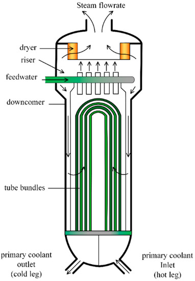
Figure 1.
Structure of the U-type SG.
SG is a highly complex, nonlinear, and time-varying inverse dynamic system. Swell and shrink are one of an SG’s dynamic characteristics. The level of SG is influenced by many factors, of which the most important are the rate of the feedwater flow and the steam flow. However, at the same time, it is also affected by the feedwater temperature, the pressure in the SG, the number of bubbles, and other factors, and the level characteristics under different powers are also quite different.
2.2. SGLCS
To keep the level of SG within a specific safe range during the operation of the nuclear power unit, the level control of SG needs to complete two main tasks. The first task is to overcome the influence of the shrink and swell effect caused by steam flow disturbance during the operation of the SG. According to the error of stream flow and water supply, the SG level can reach the setpoint in the shortest time, and the SGLCS has better dynamic characteristics. The second is to make the SG keep the relative balance between feedwater flow and steam flow and the basic constant level during stable operation, making the control system have good static characteristics [17]. To achieve the tasks, the control diagram of the SGLCS should be designed as shown in Figure 2; and the current SGLCSs generally adopts the three-impulse cascade proportional-integral-derivative (PID) control structure, which is shown in Figure 3.
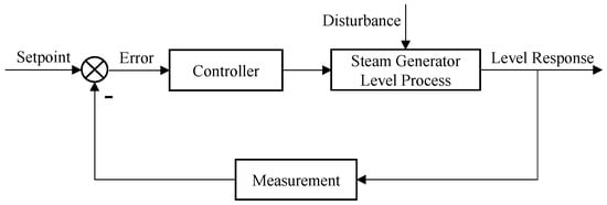
Figure 2.
Diagram of the SGLCS.
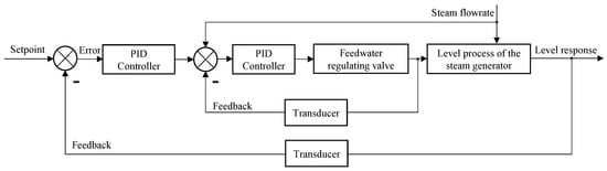
Figure 3.
Three-impulse cascade PID control structure of the SGLCS.
2.3. Performance Optimization of SGLCS
Once the SGLCS determines the control system structure, its control performance is determined mainly by the control system’s controller parameters. To optimize control performance, the relevant controller parameters of each controller need to be adjusted. The control system’s parameter optimization structure is shown in Figure 4. The choice of different parameter combinations will impact the performance of the SGLCS. A set of parameter combination solutions that can optimize the control performance of the related control system is defined as the optimal parameter combination solution. The optimization problem can be expressed as follows by converting the performance optimization described above into a mathematical statement:
where Perf represents the performance index of the control system, x represents the selected control parameter set and represents the selected range of the control parameter set, and f(x) represents the relationship between controller parameters and its corresponding control system performance index.
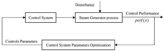
Figure 4.
Structure of control system parameter optimization.
3. Data-Driven Overall Strategy for Performance Optimization of SGLCS
According to batch characteristics of SGLCS performance optimization, a data-driven strategy framework for SG level control performance optimization is proposed, as shown in Figure 5.
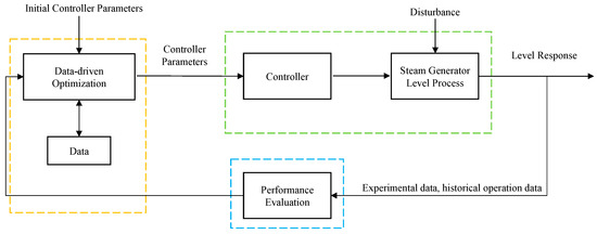
Figure 5.
Structure of data-driven performance optimization strategy for the SGLCS.
The optimization framework consists of three parts. Among them, the SG object and the control system of the NPP constitute a generalized process object; the data-driven optimization strategy consists of two parts: the performance evaluation and the data-driven optimization algorithm.
The brief introduction of each part is as follows:
(1) Generalized process object
In the actual industrial process, the generalized process object is the actual SG level process and its distributed control system (DCS). The data-driven optimization algorithm will transfer the iterative controller parameters to the DCS, modify the relevant controller parameters, and put them into the controller system. Then, the operation data are collected by DCS and transferred to the performance evaluation system. In order not to lose generality in the research process, the classical SG level model and its control model are used to substitute the actual process.
(2) Performance evaluation
The performance evaluation system receives the water level response data from the process object and stores these data. According to the characteristics of the system, the calculated value of the performance evaluation can be used to evaluate the performance of the control system corresponding to the selected control parameters. In this paper, the control system performance evaluation index uses the integral of time multiplied by the absolute error index (ITAE) to evaluate the characteristics of the step response transient curve [22], and it can be expressed as below:
In consideration of the ITAE value changing too much compared with the parameters change scale, which could make the optimization process oscillate too violently, the performance evaluation index ITAE(lg) in this paper is defined as shown in the following formula:
(3) Data-driven optimization
The data-driven optimization system receives the process data from the performance evaluation system. Historical data information generated in the optimization process is stored in order and used to guide the optimization process, improve the optimization efficiency, and reduce the optimization cost as much as possible. This paper focuses on introducing a new type of SPSA method. The improved SPSA optimization is based on the traditional SPSA optimization method and combined with the water level control characteristics of the SG to realize the adaptive adjustment of optimization step size and intelligent termination of the optimization iteration process.
4. IK-SPSA-Based Optimization Method
4.1. IK-SPSA
SPSA algorithm is a MFO methodology suitable for multi-dimensional and noisy environments [19,20]. The flowchart of the SPSA algorithm is shown in Figure 6.
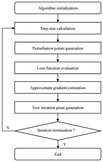
Figure 6.
Flowchart of SPSA.
Step 1: Initialization.
Determine the parameters to be optimized and their feasible areas, and select the starting point through experience or according to specific rules. Set appropriate optimization method coefficients and iteration termination conditions.
Step 2: Step size calculation.
Update step size at the current iteration batch, and the iteration step size can be calculated as below:
where k is the current iteration number. indicates the iteration step length of SPSA at the kth iteration. The perturbation step size could be calculated as follows:
where c and are coefficients of SPSA, represents the perturbation steps the size of SPSA in the kth iteration, and it will decrease with the progress of the iterative optimization process.
Step 3: Perturbation points generation.
Generate an n-dimensional perturbation vector by the Monte Carlo method, each element of which is randomly generated by Bernoulli distribution.
Assuming that the current iteration point is , then the positive perturbation point is , and the negative perturbation point is .
Step 4: Loss function evaluation.
In the kth iteration, evaluate the loss functions of iteration points , positive perturbation points, and negative perturbation points .
Step 5: Gradient approximation calculation.
Gradient approximation can be calculated according to positive and negative perturbation points and their corresponding loss function values. The approximate formula of the gradient is as below:
Step 6: New iteration point generation.
The new iteration point is generated by and according to the following formula:
The traditional SPSA algorithm has high efficiency. However, because of its fixed step size mechanism, the related parameters of step sizes cannot be adjusted adaptively. If the step size is too small, the optimization process will be slowed down, and when the step size is too large, it will cross the optimal solution and cause oscillation in the optimization process.
To solve the above problems and make the SPSA algorithm more efficient and accurate, the following effective improvement schemes are put forward by using the data-driven idea combined with the adjacent iteration points in historical information:
Firstly, the current optimization process status is evaluated based on data-driven historical information. Hence, the SPSA could adjust its iteration step size according to the status evaluation. Thus, it obtains an adaptive ability in the optimization process.
Secondly, integrated adaptive compensation factors in SPSA will adaptively adjust the next iteration step size according to the current optimization process status. Hence, an improved algorithm (knowledge-informed simultaneous perturbation stochastic approximation, IK-SPSA) is formed, combining the above two ideas and the regular pattern of historical information. It can adaptively adjust the step size according to the current optimization process status and effectively improve the optimization efficiency of SPSA.
The flowchart of the IK-SPSA algorithm is shown in Figure 7, and the specific implementation steps are as follows:
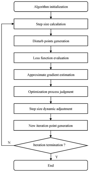
Figure 7.
Flowchart of the IK-SPSA.
Steps 1–5 are the same as the steps of SPSA.
Step 6: Optimization process judgment.
To identify the status of the optimization process, a large number of historical iterative optimization process data are compared with typical optimization process trajectories.
According to the analysis, it is concluded that five kinds of local optimization process status are: rapid local descent, local deceleration descent, local uniform descent, local concave oscillation, and local convex oscillation, as shown in Figure 8.
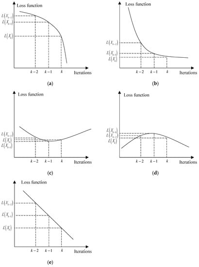
Figure 8.
Diagram of typical local optimization scenes: (a) Local rapid descent scenario; (b) local slow descent scenario; (c) local concave oscillation scenario; (d) local convex oscillation scenario; (e) local uniform descent scenario.
To identify the process status in the optimization process, the adjacent historical iteration information is used to obtain the judgment factor. It is used to judge the current optimization process status. The judgment factor can be denoted as:
where represents information set of point loss function of successive three iterations; is weighting factor; is judgment factor of current optimization status. The relationship between that judgment factor and the status of the optimization process is as follows:
(1) If the optimization process is currently in a rapid decline stage, then the judgment factor is . It shows that the current optimization increment is large, and the optimization process can be accelerated, and the appropriate step size can be increased by the compensation factor to accelerate the optimization process;
(2) If the optimization process is in the slow descending stage at this time, then the judgment factor is indicating that the optimization increment is small and close to the local optimum, and the optimization process can be slowed down by reducing the appropriate step size through the compensation factors;
(3) When the optimization process is in a critical status, that is, the constant-speed descending stage, . Keep the current step size without adjustment.
(4) If the optimization process is in a status of local oscillation at present, the optimization process is close to the local optimum at this time, to make the optimization process converge. The compensation factor reduces the size of the appropriate step size to slow down the optimization process to ensure its convergence.
Step 7: Dynamic adjustment of step size.
Adjust the current step size according to the judgment factor as follows:
The sign of is obtained from the following formula by the loss function value of adjacent historical iteration points:
where is a symbolic function. is obtained from the parameter set of adjacent iteration points of the optimization process, as shown in the following formula:
Step 8: New iteration point generation.
4.2. Iteration Termination Control
MFO based on data-driven not only needs the rationality of iterative step optimization but also needs a reasonable mechanism to realize the timely termination of the iterative optimization process [15]. In the process of optimization, convergence is its important characteristic and evaluation index. The traditional SPSA realizes iteration termination according to the fixed maximum number of iterations. To improve the optimization efficiency and avoid exchanging multiple iteration costs for smaller optimization results, it is necessary to analyze the historical iteration information to realize the timely termination of the iteration process. Figure 9 is the control flowchart of iteration termination.
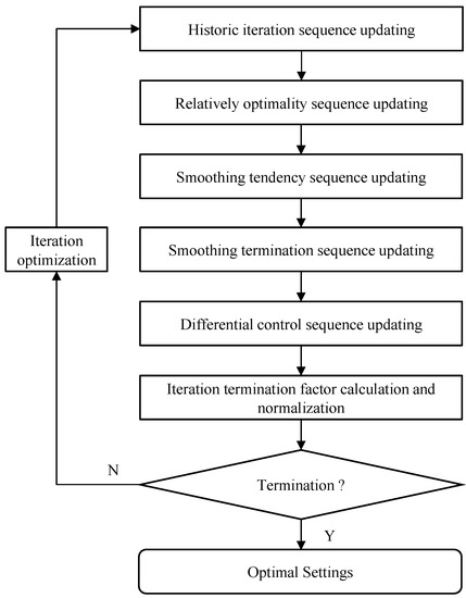
Figure 9.
Flowchart of iteration termination control.
The implementation can be divided into the following five steps:
Step 1: Historical iteration sequence updating.
The historical iteration function sequence is a self-increasing sequence that stores the function values of all historical iteration points. When a new iteration point is generated, the iteration point function value is updated to the sequence.
Step 2: Relative optimality sequence updating.
The historical iteration sequence will be sorted according to the control performance of alliteration points. A relatively optimal iteration sequence, is iteratively formulated based on the best point at each iteration.
Step 3: Smoothing tendency sequence updating.
To obtain the iterative process trend, the relatively optimal sequence is smoothed by the moving average method to obtain the smoothed trend sequence , as shown in Equation (13).
where n is the dimension of the parameter and is the smoothing coefficient.
Step 4: Smoothing termination sequence updating.
Further, smooth the smoothed trend sequence to obtain termination sequence for termination control. is a monotone decreasing sequence based on the trend sequence , as in Equation (14).
Step 5: Differential control sequence updating.
Differential control sequence, , is formulated as below:
Step 6: Iteration termination factor calculation and normalization.
To evaluate the relative progress of optimization, the termination factor is defined as shown in the following formula:
where indicates the ratio of control performance improvement to current point performance. Considering the consistency of the termination factor, it is necessary to normalize the termination factor to obtain a general factor independent of the problem. The normalization is shown as in Equation (17).
Step 7: Iteration termination.
When is small enough, that is , ( is the allowable error), and to avoid premature termination of iteration due to accidental factors in the iteration process, it is further verified, so the iteration termination rule is defined as:
is the repetition coefficient that can be set by the engineer, indicates a counter representing the number of iterations that satisfies the former tolerance. When the termination condition is met, the optimization process will be terminated and the optimal solution will be obtained.
5. Results and Discussions
5.1. Simulation Experiment Platform
The SG level change process is time-varying, highly complex, and has an obvious swell and shrink phenomenon. Considering the particularity of nuclear power operation safety, it is difficult to carry out online experiments on actual nuclear power units. In this paper, the piecewise linear mathematical model of SG level proposed by E. Irving is used as the simulation experiment platform [23].
E. Irving’s SG level model is widely adopted in the research of SG level control, and its transfer function is as follows:
where Y is the level of the SG; is the feedwater flow and is the steam flow; is a constant coefficient; is the delay time; T is the oscillation period, and the unit is s; s is Laplace transform operator.
E. Irving’s model is a piecewise linear model, and the parameters change in different power segments. The state-space expression of the SG level model is shown in the following:
where is the feedwater flow; is the steam flow; and is the water level.
The feedwater flows step response and steam flow step response of the simulated E. Irving’s model under different powers are shown in Figure 10 and Figure 11, respectively. It can be seen from Figure 10 and Figure 11 that with the increase of power, the swell and shrink effects weaken, which is consistent with the actual SG level response phenomenon. Moreover, when the power reaches 30%, the step response curve of feedwater flow has apparent oscillation, which shows that E. Irving’s model can better reflect the actual SG’s false level and mechanical oscillation. Furthermore, at the same power, the level value of the SG finally decreased due to the increase of steam flow rate is equal to the level value of the SG finally increased due to the increase of feedwater flow rate. The actual SG can keep the level unchanged when the feedwater flow rate and steam flow rate are equal.
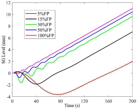
Figure 10.
Curve of level response for step flowrate in feedwater at different powers.
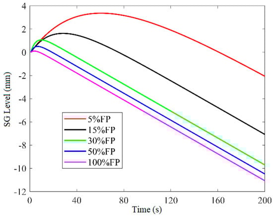
Figure 11.
Curve of level response for step flowrate in steam at different powers.
5.2. Experimental Setup
The SG level model adopts the piecewise linear mathematical model of the SG level proposed by E. Irving as the simulation experiment platform. As shown in Figure 3, the SG level control system adopts the three-impulse cascade PID control scheme in 5% full power (FP), 30% FP, 50% FP, and 100% FP. The control system includes six controller parameters: the primary PID and the auxiliary PID. In this paper, these six controller parameters are selected as optimization variables, and these six controller parameters are set as , the maximum number of iterations is 40. As NPPs have special requirements for safety, the constraint range of control parameters should be within the stable range of control system. In reality, the constraint range can be selected through the experience of engineers. Detailed description and constraints of optimized variables are shown in Table 1, and system parameters are shown in Table 2.

Table 1.
Controller parameters settings of the cascade PID control system.
Table 2.
Parameters settings of cascade PID control system.
5.3. Effectiveness Test
IK-SPSA does not change the basic framework of the SPSA method, so its convergence is consistent with the SPSA method. As a stochastic search algorithm, its effectiveness can be demonstrated by its principal design and numerical statistical test. This method has been widely used and recognized by academy and industry [19,20,21]. Without losing generality, the Monte Carlo method is used to randomly select the initial points of different powers. Adjust the control system parameters to the above control parameters. The IK-SPSA optimization strategy is implemented in the experiment. The optimization process and results are recorded as shown in Figure 12, Figure 13, Figure 14 and Figure 15 below.
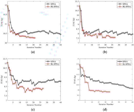
Figure 12.
Trajectories of iteration: (a) 5% FP; (b) 30% FP; (c) 50% FP; (d) 100% FP.
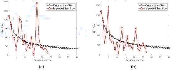
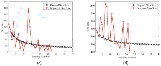
Figure 13.
Trajectories of step size change: (a) 5% FP; (b) 30% FP; (c) 50% FP; (d) 100% FP.
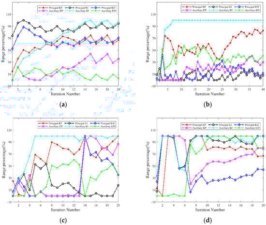
Figure 14.
Trajectories of optimizing parameters change: (a) 5% FP; (b) 30% FP; (c) 50% FP; (d) 100% FP.
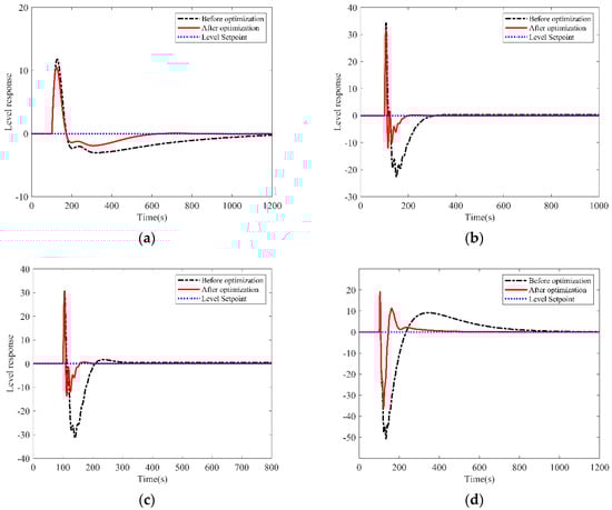
Figure 15.
Curve of water level change before and after optimization: (a) 5% FP; (b) 30% FP; (c) 50% FP; (d) 100% FP.
(1) Trajectories of iteration
From Figure 12, with the advancement of the optimization process, the ITAE index continues to drop significantly, which also means that the control system’s performance has been significantly improved. Moreover, the whole optimization process only needs more than 20 times iterations, which means that IK-SPSA can achieve the optimization goal in a limited number of times and IK-SPSA can realize intelligent iteration termination, avoiding unnecessary iteration cost waste. Figure 12 shows that IK-SPSA has certain advantages over SPSA. IK-SPSA can find the optimal value faster, which verifies the effectiveness of the improved mechanism to a certain extent.
(2) Trajectories of step size change
It can be seen from Figure 13 that the overall trend of the improved step size of IK-SPSA is consistent with the continuous decrease with the increase of iteration times, thus avoiding the oscillation near the optimal value. In addition, there will be some fluctuations in the step size, indicating that IK-SPSA can judge the current optimization process status and adjust the step size accordingly according to the current optimization process status. IK-SPSA can adaptively adjust the step size to find the optimal value.
(3) The changing track of algorithm optimization parameters
According to the characteristics of the IK-SPSA optimization strategy, the control system parameters will be improved in parallel with the progress of iterative optimization. The change of these key controller parameters is accompanied by the continuous improvement of control system performance. The trajectories of the controller parameters can be observed in Figure 14. It can be found that with the advancement of the optimization process, the six key controller parameters will undergo random parallel perturbation and continuous dynamic change.
(4) Comparison of the level of SGLCS before and after optimization
When the iteration termination control conditions are met, the optimization method terminates in time and finds an optimal control parameter point. To show the change in the control system performance before and after the optimization process and to prove the effectiveness of the optimization method, Figure 15 draws the transient response curves of the control system water level at the initial point and the optimal working parameter point during the optimization process. The dotted line is the water level target setting value. The solid line curve is the water level curve before optimization. The dotted line is the water level curve after optimization. Compared with the control system before optimization, the maximum deviation of the optimized control system under different power is reduced by 2%, 3.2%, 2.1%, and 27%, respectively. The peak time is reduced by 4.7%, 10%, 9.8%, and 34%, respectively; The transient time is reduced by 50%, 60%, 75%, and 71%, respectively. The response performance of the optimized control system is greatly improved, which also reflects the effectiveness of the IK-SPSA method.
(5) IK-SPSA iterative Trajectories at different initial points
To verify the effectiveness of the IK-SPSA method from different initial points, three different initial points were selected as initial values in the experiment. Under these three different initial points, the optimized trajectories based on IK-SPSA are shown in Figure 16 below. All three optimization experiments show similar performance, which can be completed under a few iterative experiments, which also proves the effectiveness of the optimization method for performance at different initial points.
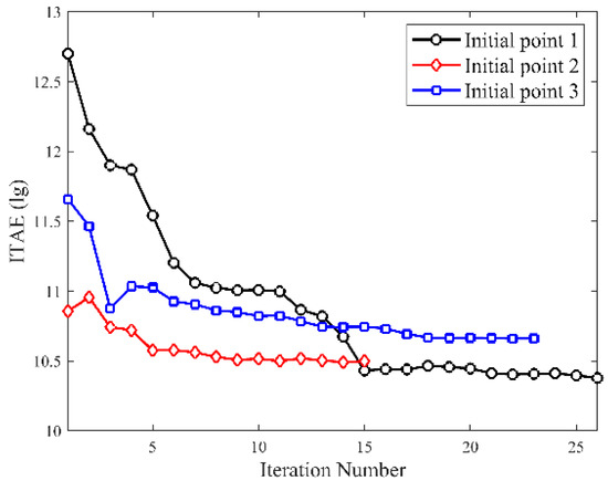
Figure 16.
Trajectories of iterative at different initial points.
5.4. Efficiency Test
The above tests show that both the traditional SPSA strategy and the improved IK-SPSA strategy are effective in optimizing the SG level control performance. To further test the performance difference between SPSA and improved IK-SPSA, the iterative termination mechanism was introduced for both algorithms, and batch experiments with the same initial point and different initial points were carried out under the same other working conditions.
5.4.1. Experimental Design
One thousand groups of experimental tests were conducted with the same control parameters as the initial point in 100%FP.
The sequential Latin square sampling method was used to design experiments at different initial points. Each parameter was divided into ten levels according to its value interval. Ten independent sampling points were randomly generated by the Monte Carlo method for a single Latin square sampling. In this test, the batch number of sequential Latin squares was set to 100. That is, 100 times of Latin square sampling were repeated during the experiment, and ten random samples were taken for each Latin square sampling, resulting in a total of 1000 sample points. Under the initial values of these sample points, the performance indexes of the optimization methods were counted to evaluate the performance of the two methods.
5.4.2. Efficiency Analysis
Figure 17 and Figure 18 show the distribution of the average number of iterations under the Latin square sampling experiment of each batch.
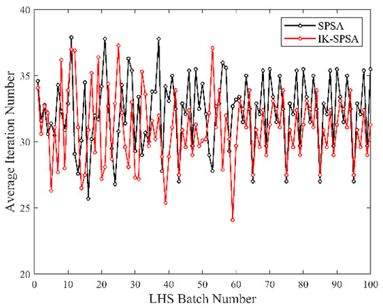
Figure 17.
Average iteration number distribution at the same initial point.
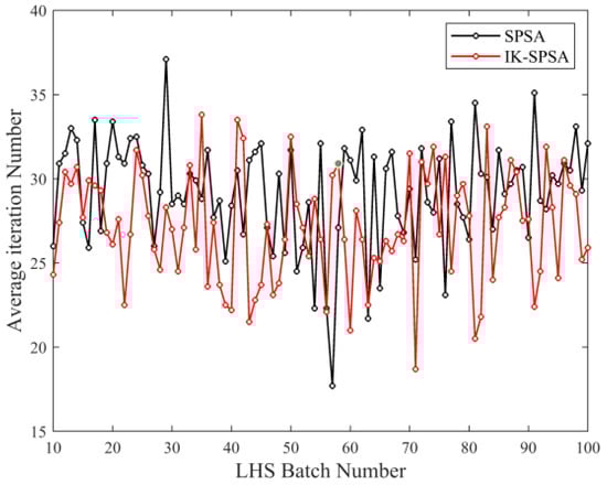
Figure 18.
Average iteration number distribution at different initial points.
Experimental results show that IK-SPSA and SPSA have strong adaptive termination control ability because of the addition of the iterative termination control mechanism, and the number of iterations presents a dynamic distribution. The IK-SPSA optimization process can be terminated with fewer iterations, and the optimization iteration cost is reduced compared with the traditional SPSA strategy.
Figure 19 and Figure 20 show the average iteration final value distribution under each batch’s Latin square sampling experiment.
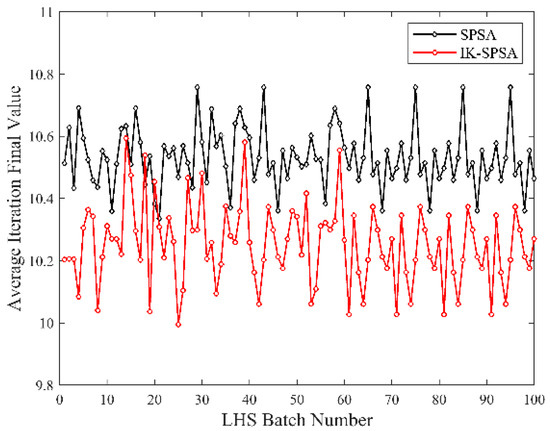
Figure 19.
Average iteration final value distribution at the same initial point.
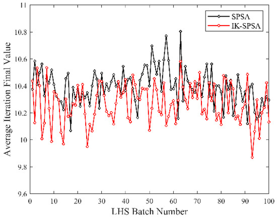
Figure 20.
Average iteration final value distribution at different initial points.
The experimental results show that due to the random perturbation characteristics of the SPSA algorithm, the iterative final value presents a dynamic distribution. Overall, the IK-SPSA optimization process can get a lower iteration final value, and the optimization performance is improved compared with the traditional SPSA strategy.
Sequential Latin square experimental design can provide trend trajectories analysis perspective to optimize the dynamic change of performance. Figure 21 and Figure 22 show the dynamic change track of the accumulated average iteration times of IK-SPSA. With the advance of sequential Latin square batches, in the initial status, the average iteration times may deviate significantly from the statistical values because the number of experimental samples is insufficient. With the proceeding of Latin hypercube sampling (LHS) batches, the number of samples covered increases gradually. Correspondingly, the cumulative performance indices converged to a stable value gradually. The average performance in the feasible region could exhibit convergence characteristics under the cumulative effect, and the variability in the performance of the methods is thus eliminated. This could reveal the relative performance between the two methods. Through 1000 groups of experiments, under the same initial point and different initial points, the average iteration times of IK-SPSA are 31 and 27, respectively, and the average iteration times of SPSA are 32.2 and 29, respectively. Compared with the typical SPSA method, the iteration times of IK-SPSA strategy are reduced by 3.7% and 6.9%, respectively. When compared to the typical SPSA approach, the iteration times of the IK-SPSA strategy are shorter.
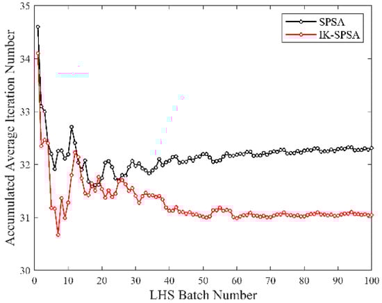
Figure 21.
Accumulated average iteration number distribution at the same initial point.
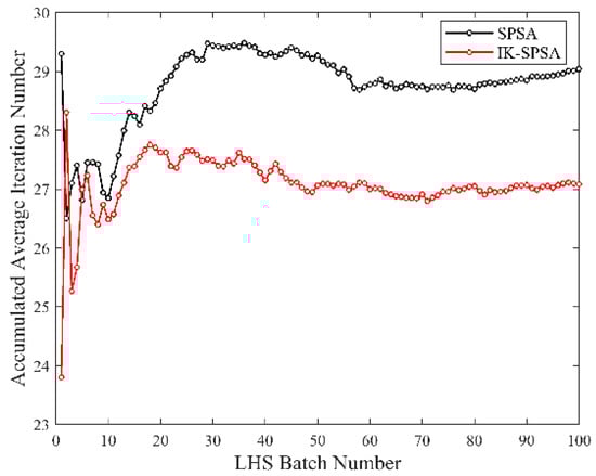
Figure 22.
Accumulated average iteration number distribution at different initial points.
The dynamic change track of the accumulated average iteration final value of IK-SPSA is shown in Figure 23 and Figure 24. Through 1000 groups of experiments, under the same initial point and different initial points, the average iterative final values of IK-SPSA are 10.25 and 10.26, and the average iterative final values of SPSA are 10.52 and 10.39, respectively. Compared with the typical SPSA method, the iterative final value of IK-SPSA strategy is reduced by 2.6% and 1.3%, respectively. It can be seen that the method based on IK-SPSA is superior to the traditional SPSA method and can obtain better control parameters.

Figure 23.
Accumulated average iteration final value distribution at same initial point.
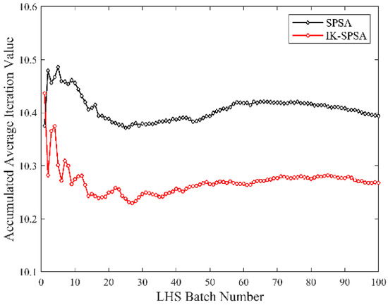
Figure 24.
Accumulated average iteration final value distribution at different initial points.
6. Conclusions
A revised simultaneous perturbation stochastic approximation (SPSA), IK-SPSA, was proposed in this study to optimize the SGLCS controller parameters via only direct control system performance measurements. The historical information generated during the optimization process was utilized to enhance the optimization efficiency. Hence, two critical mechanisms were constructed to form this novel data-driven optimization strategy. The real time step size tuning mechanism could sense the current optimization status and thus adaptively tune the next iteration step size. The termination control mechanism could evaluate the progress of the optimization from a holistic perspective and thus could terminate the optimization intelligently to avoid unnecessary iteration costs. Moreover, the IK-SPSA strategy was adjusted adaptively according to the characteristics of the performance optimization of the SGLCS. This strategy was verified on a typical SGLCS simulation platform. A series of systemic experiments were designed and conducted. The effectiveness and the efficiency of the IK-SPSA were both tested. The experimental results indicated that the IK-SPSA-based performance optimization strategy for the SGLCS was effective and the efficiency was better relative to the traditional methods and can improve the stability, safety, and economy of SGLCS. Although the knowledge-informed MFO method uses the historical data of online iteration to improve the optimization efficiency, prior historical data is not considered. Next, we will further consider prior historical data to improve the optimization efficiency of the knowledge-informed MFO method.
Author Contributions
Conceptualization, P.G., X.K., C.S., H.L. and J.L.; data curation, P.G. and X.K.; formal analysis, X.K.; funding acquisition, X.K., C.S., H.L. and J.L.; investigation, X.K. and C.S.; methodology, X.K. and C.S.; project administration, X.K., C.S., H.L. and J.L.; resources, X.K., C.S. and H.L.; software, P.G. and X.K.; supervision, X.K., C.S. and H.L.; validation, P.G. and X.K.; visualization, P.G. and X.K.; writing—original draft, P.G. and X.K.; writing—review and editing, X.K., P.G., C.S. and H.L. All authors have read and agreed to the published version of the manuscript.
Funding
This research was funded by the program of the State Key Laboratory of Nuclear Power Safety Monitoring Technology and Equipment of China (K-A2020.412), and the Natural Science Foundation of Fujian Province, grant numbers 2021J011205, 2020J01284 and 2018J01564.
Institutional Review Board Statement
Not applicable.
Informed Consent Statement
Not applicable.
Data Availability Statement
Not applicable.
Conflicts of Interest
The authors declare no conflict of interest.
Abbreviations
| DCS | distributed control system |
| FP | full power |
| IK-SPSA | knowledge-informed simultaneous perturbation stochastic approximation |
| ITAE | integral of time multiply by absolute error |
| LHS | Latin hypercube sampling |
| MFO | model-free optimization |
| NPP | nuclear power plant |
| PID | proportional-integral-derivative |
| SG | steam generator |
| SPSA | simultaneous perturbation stochastic approximation |
| SGLCS | steam generator level control system |
References
- Javadi, M.A.; Abhari, M.K.; Ghasemiasl, R.; Ghomashi, H. Energy, exergy and exergy-economic analysis of a new multigeneration system based on double-flash geothermal power plant and solar power tower. Sustain. Energy Technol. Assess. 2021, 47, 1–25. [Google Scholar] [CrossRef]
- Javadi, M.A.; Khalaji, M.; Ghasemiasl, R. Exergoeconomic and environmental analysis of a combined power and water desalination plant with parabolic solar collector. Desalination Water Treat. 2020, 193, 212–223. [Google Scholar] [CrossRef]
- Zhang, M.; Zhang, Z. Necessity and Feasibility Study of Nuclear Power Development under COP 26 Carbon Reduction Goal. Nucl. Saf. 2022, 21, 26–31. [Google Scholar]
- Ansarifar, G.R.; Talebi, H.A.; Davilu, H. Adaptive estimator-based dynamic sliding mode control for the water level of nuclear steam generators. Prog. Nucl. Energy 2012, 56, 61–70. [Google Scholar] [CrossRef]
- Rahimi-Adli, K.; Leo, E.; Beisheim, B.; Engell, S. Optimisation of the Operation of an Industrial Power Plant under Steam Demand Uncertainty. Energies 2021, 14, 7213. [Google Scholar] [CrossRef]
- Xu, Y.; Chen, J.; Yu, H.; Wang, Z. Research on Feedforward Compensation for Steam Generator Level Control System Manual/Automatic Switch. Hedongli Gongcheng/Nucl. Power Eng. 2021, 42, 140–144. [Google Scholar]
- Ma, S. Trip analysis and online diagnosis regulation for loosing water level control of the PWR steam generator. Nucl. Sci. Eng. 2009, 29, 328–332. [Google Scholar]
- Salehi, A.; Safarzadeh, O.; Kazemi, M.H. Fractional order PID control of steam generator water level for nuclear steam supply systems. Nucl. Eng. Des. 2019, 342, 45–59. [Google Scholar] [CrossRef]
- Zhang, D.; Cai, W.; Xie, C.; Liu, P.; Liu, C. Research on Automatic Optimization Software for PID Parameters of Nuclear Power Digital Control System. Nucl. Sci. Eng. 2020, 41, 77–81. [Google Scholar]
- Zeng, D.; Zheng, Y.; Luo, W.; Hu, Y.; Cui, Q.; Li, Q.; Peng, C. Research on Improved Auto-Tuning of a PID Controller Based on Phase Angle Margin. Energies 2019, 12, 1704. [Google Scholar] [CrossRef]
- Goran, K.S.; Zeljko, M.D. Water Level Control in the Thermal Power Plant Steam Separator Based on New PID Tuning Method for Integrating Processes. Energies 2022, 15, 6310. [Google Scholar] [CrossRef]
- Wu, S.; Wang, P.; Wan, J.; Wei, X.; Zhao, F. Parameter Optimization for AP1000 Steam Generator Feedwater Control System Using Particle Swarm Optimization Algorithm. In Proceedings of the 24th International Conference on Nuclear Engineering, Charlotte, NC, USA, 26–30 June 2016; p. V001T04A006. [Google Scholar]
- Puchta, E.; Bassetto, P.; Biuk, L.; Filho, M.I.; Converti, A.; Kaster, M.; Siqueira, H. Swarm-Inspired Algorithms to Optimize a Nonlinear Gaussian Adaptive PID Controller. Energies 2021, 14, 3385. [Google Scholar] [CrossRef]
- Kong, X.; Zheng, D. A Knowledge-Informed Simplex Search Method Based on Historical Quasi-Gradient Estimations and Its Application on Quality Control of Medium Voltage Insulators. Processes 2021, 9, 770. [Google Scholar] [CrossRef]
- Kong, X.; Guo, J.; Zheng, D.; Yang, J.; Zhang, J.; Fu, W. An improved-SPSA quality control method for medium voltage insulator SPSA. Gao Xiao Hua Xue Gong Cheng Xue Bao/J. Chem. Eng. Chin. Univ. 2020, 34, 1500–1510. [Google Scholar]
- Kong, X.; Xu, W.; Ma, Z. A novel method for controllers parameters optimization of steam generator level control. In Proceedings of the 21st International Conference on Nuclear Engineering, Chengdu, China, 29 July–2 August 2013. [Google Scholar]
- Kong, X.Z.J.; Xiao, Y.; Qian, L.; Su, L.; Chen, B.; Xu, M. Performance optimization for steam generator level control based on a revised simultaneous perturbation stochastic approximation algorithm. In Proceedings of the 2018 3rd International Conference on Intelligent Green Building and Smart Grid (IGBSG), Yi-Lan, Taiwan, 22–25 April 2018; pp. 1–4. [Google Scholar]
- Geng, P.; Shi, C.; Kong, X.; Liu, H.; Liu, J.; Jiang, S. SPSA-based Performance Optimization Method for Steam Generator MPC Level Control System. Hedongli Gongcheng/Nucl. Power Eng. 2022; 1–8, in press. Available online: http://kns.cnki.net/kcms/detail/51.1158.TL.20220906.0909.002.html (accessed on 10 July 2022).
- Radac, M.B.; Precup, R.E.; Petriu, E.M.; Preitl, S. Application of IFT and SPSA to servo system control. IEEE Trans. Neural Netw. 2011, 22, 2363–2375. [Google Scholar] [CrossRef] [PubMed]
- Spall, J.C. Introduction to Stochastic Search and Optimization. Estimation, Simulation, and Control. IEEE Trans. Neural Netw. 2007, 18, 964–965. [Google Scholar]
- Xun, Z.; Spall, J.C. A modified second-order SPSA optimization algorithm for finite samples. Int. J. Adapt. Control. Signal Process. 2002, 16, 397–409. [Google Scholar]
- Kong, X.; Shi, C.; Liu, H.; Geng, P.; Liu, J.; Fan, Y. Performance Optimization of a Steam Generator Level Control System via a Revised Simplex Search-Based Data-Driven Optimization Methodology. Processes 2022, 10, 264. [Google Scholar] [CrossRef]
- Irving, E.; Miossec, C.; Tassart, J. Towards efficient full automatic operation of the PWR steam generator with water level adaptive control. In Boiler Dynamics and Control in Nuclear Power Stations 2; Bournemouth; Thomas Telford Publishing: London, UK, 1980; pp. 309–329. [Google Scholar]


Publisher’s Note: MDPI stays neutral with regard to jurisdictional claims in published maps and institutional affiliations. |
© 2022 by the authors. Licensee MDPI, Basel, Switzerland. This article is an open access article distributed under the terms and conditions of the Creative Commons Attribution (CC BY) license (https://creativecommons.org/licenses/by/4.0/).