
Performance Comparison of Control Strategies for Plant-Wide Produced Water Treatment


Abstract
:1. Introduction
- The performance of the hydrocyclone is dependent on and its variations, which is determined from the control of the separator tank;
- Aggressive control will propagate disturbances to , which affects the performance of the hydrocyclone;
- As is strongly related to , the actions of the controller commonly cause the controller to saturate ;
- It is proven that and is proportional. However, there exists operational conditions where and separation performance is uncorrelated.
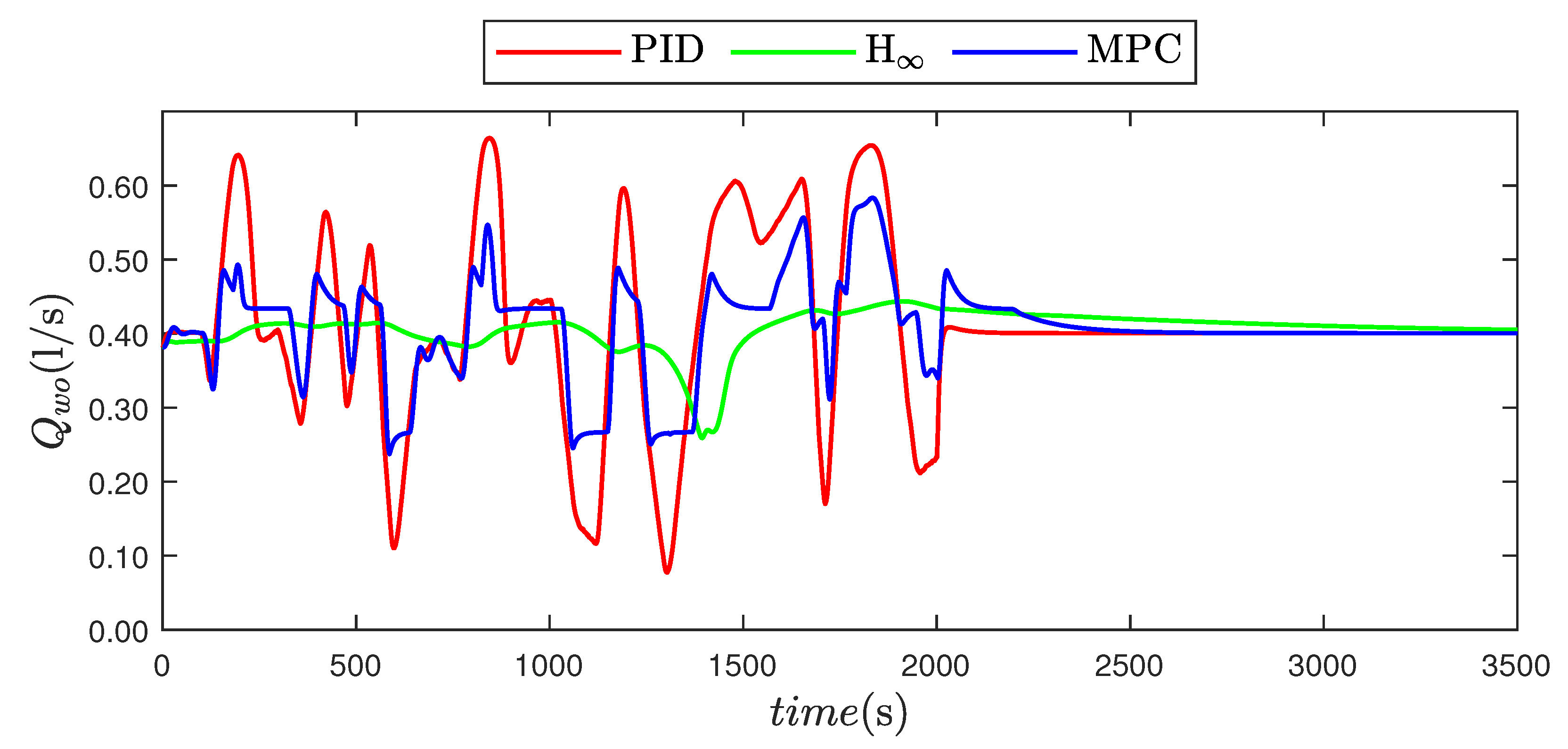
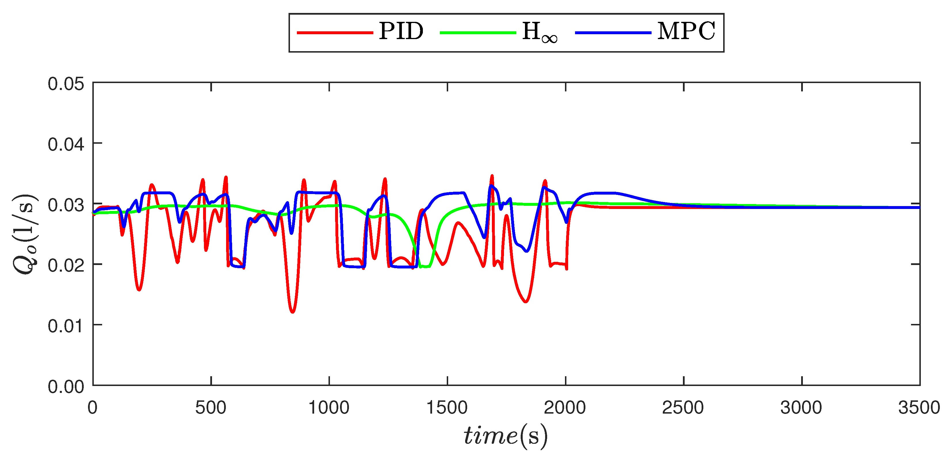
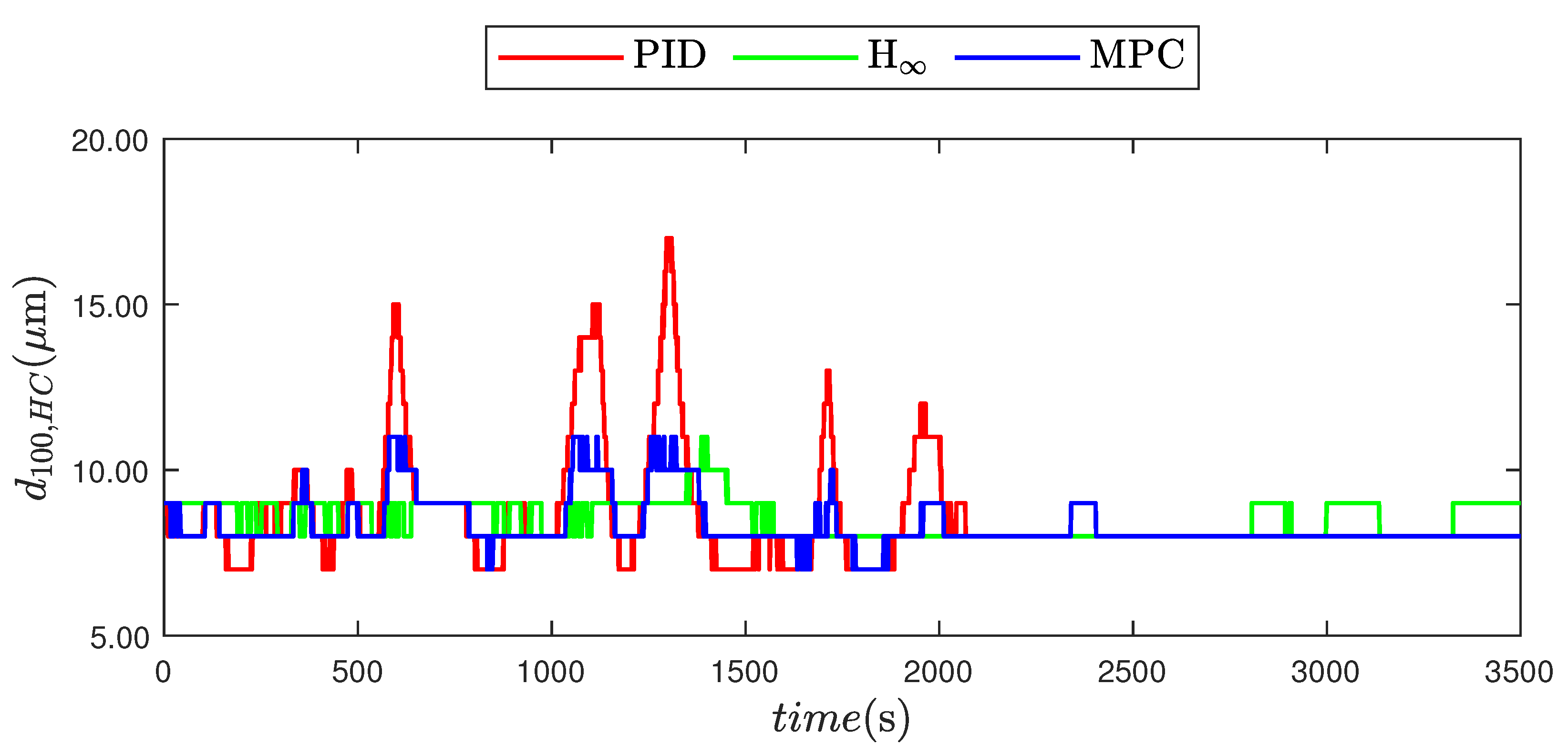
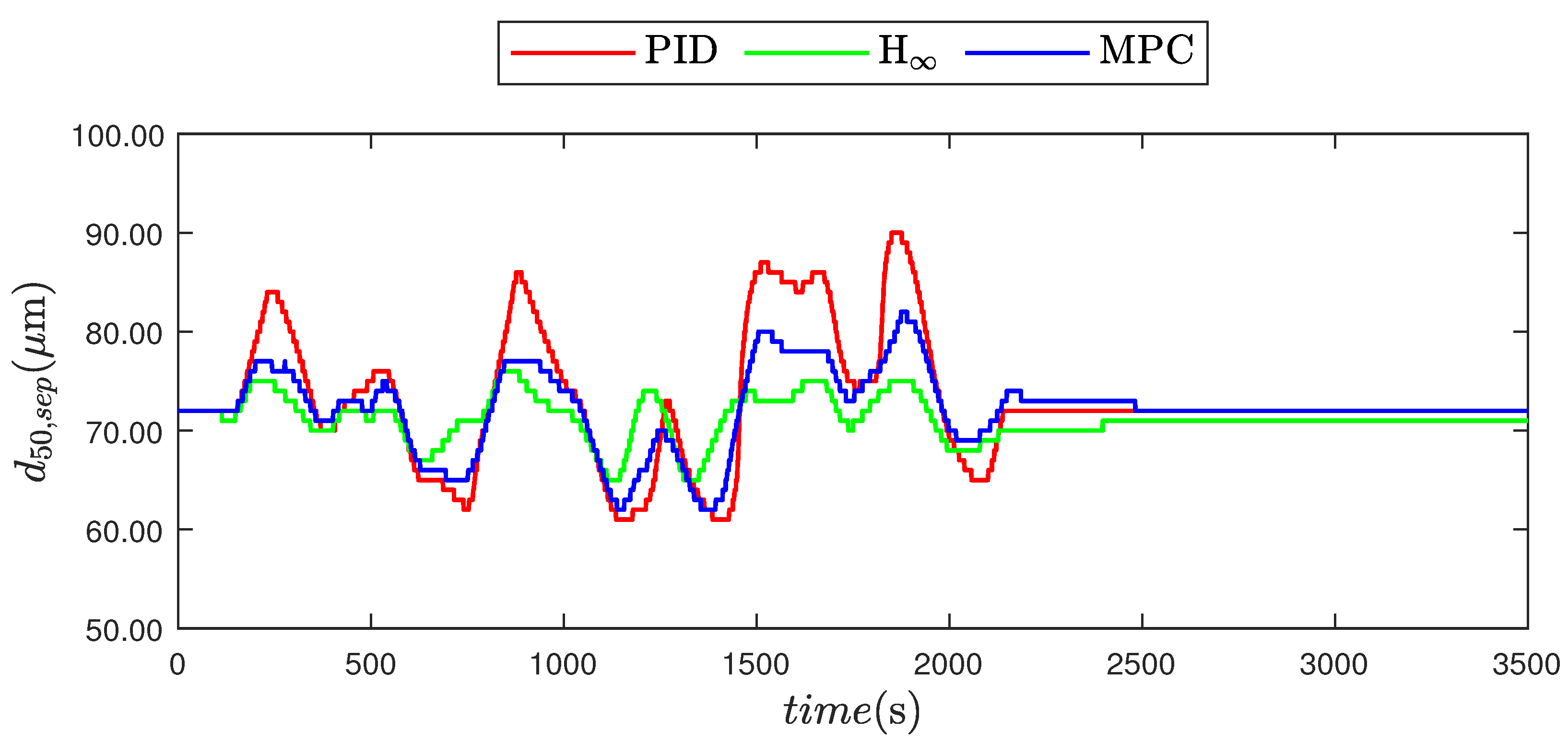
- The PID solution will propagate inflow fluctuations to the hydrocyclone and have the worst deoiling performance.
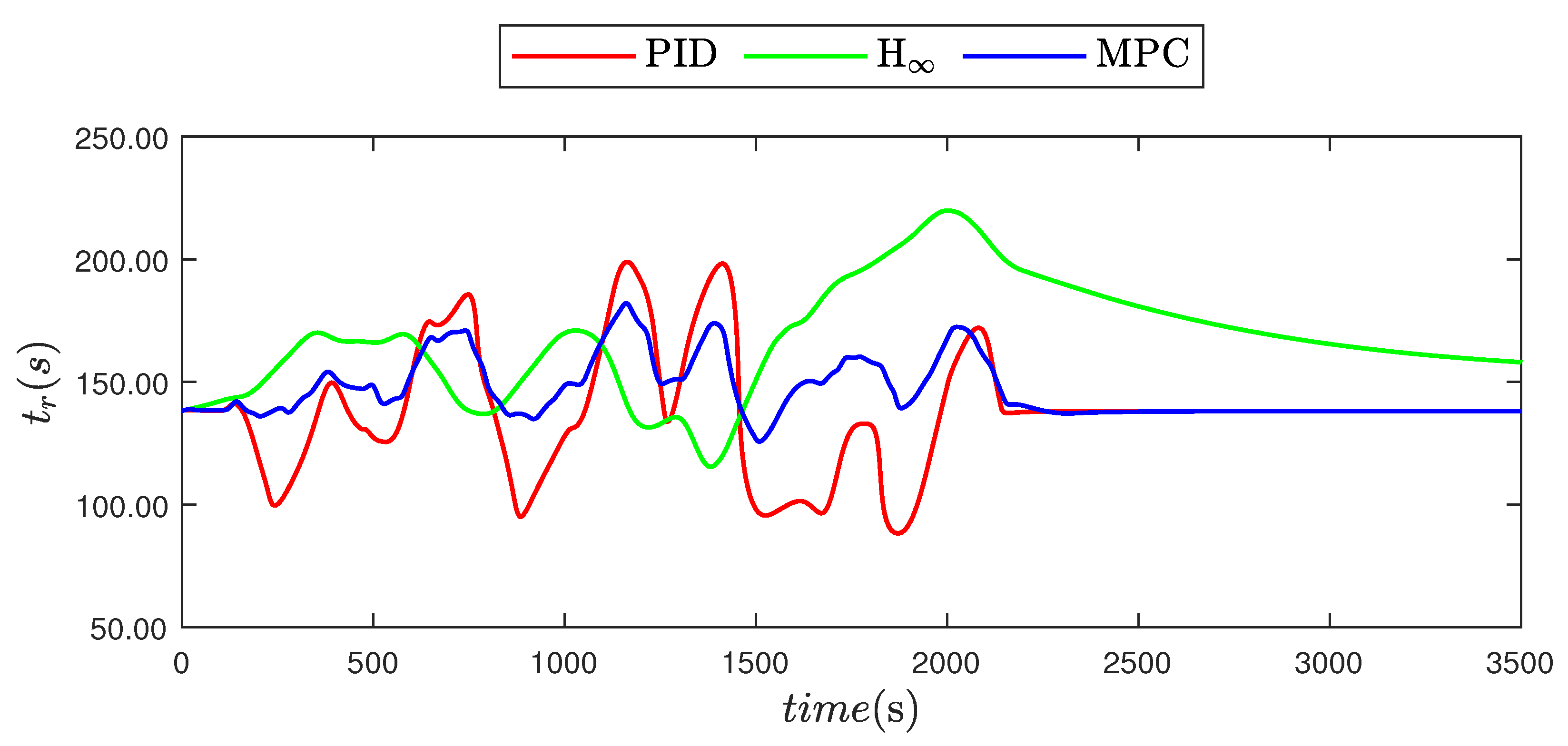
- The and MPC solutions will buffer the inflow fluctuations in the separator and have higher deoiling performance than the PID solution.
- The and MPC solutions will only differ when the constraints of the MPC solution are active, at which point it is unknown which solution will have the higher deoiling performance.
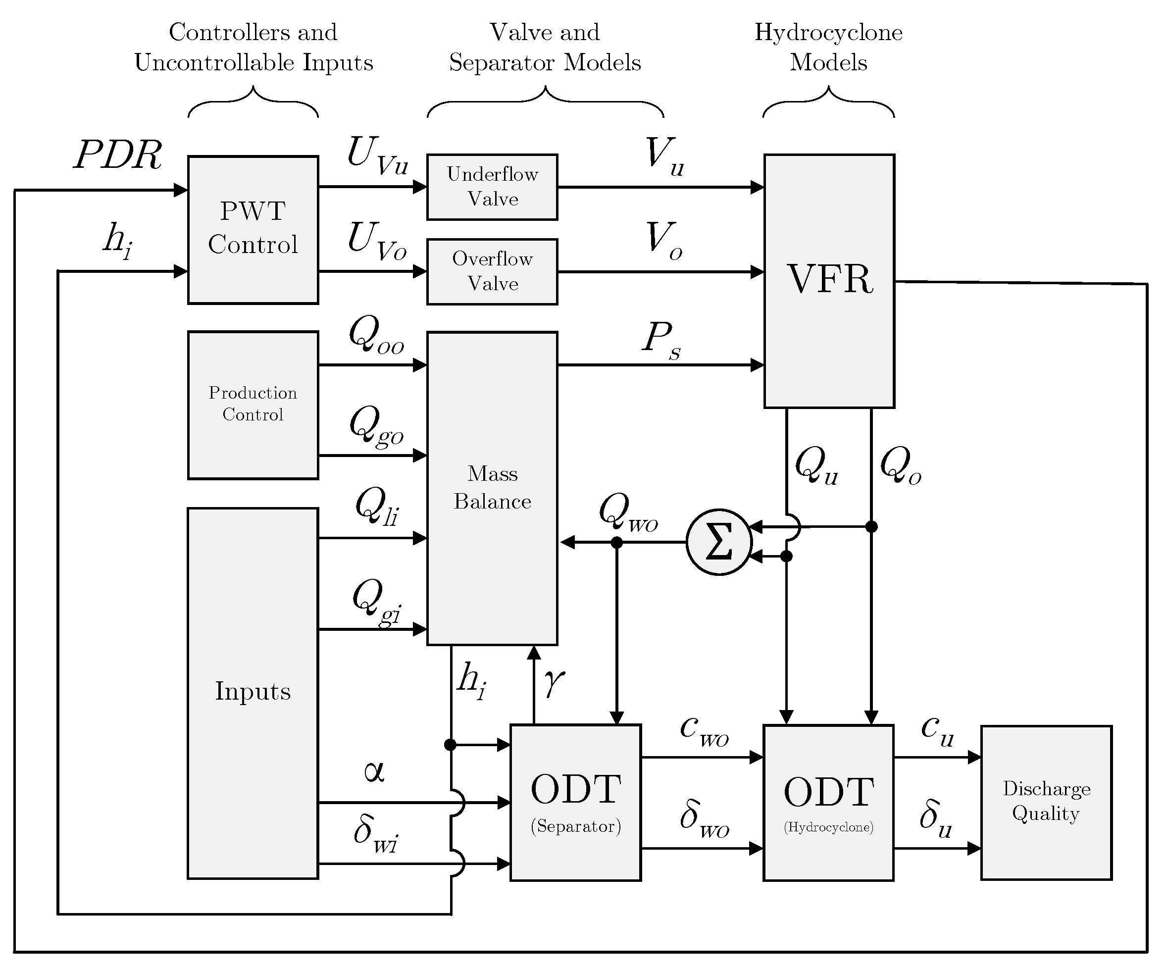
2. Methods
2.1. Grey-Box Modeling
2.1.1. Separator Tank
- Superficial velocity of water through the separator’s water phase is now calculated from the water outlet flow rate. This change reduces the reliance on arbitrary parameters as described in Equation (8).
- The residence time is now calculated for each sample by summing the horizontal distance traveled for each sample going backwards in time starting from the water outlet ending at the input flow region. The residence time is then the total number of samples required to travel that distance multiplied by the sample time. This change more accurately estimates the residence time as described in Equations (9) and (10).
- Initial WiO and OiW ratios, and , are now parameters instead of inputs, as both are assumed constant to simplify the simulation model.
- Initial WiO ratio parameter is set to 0, and there is no longer a need for a water droplet distribution. This work does not concern water in the oil phase and is therefore excluded in the simulation model.
Mass Balance
Oil Droplet Trajectory
2.1.2. Hydrocyclone
Virtual Flow Resistance
Oil Droplet Trajectory
2.2. Control Candidates
2.2.1. PID Control
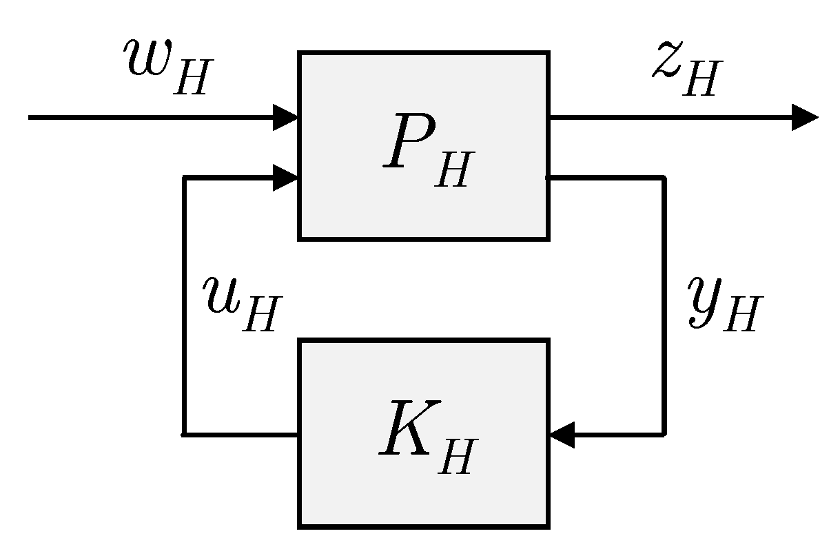
2.2.2. Control
2.2.3. MPC
- Input disturbance model updated to the transfer function: .
- Measurement noise model for has been updated to an assumed standard deviation of 0.51.
- Measurement noise model for has been updated to an assumed standard deviation of 59.1.
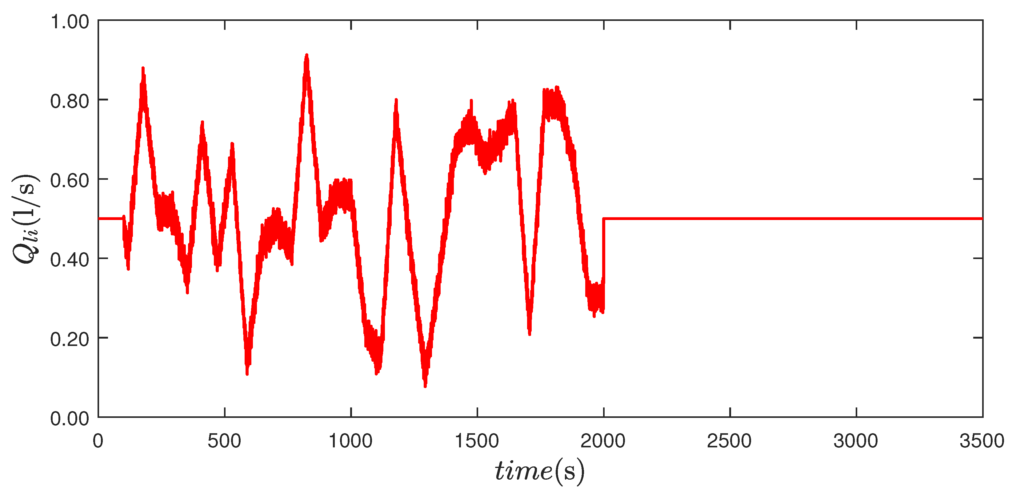
2.3. Simulation Scenario
- The set-point for the separator gas pressure is 7 bar, as this was the operation condition during system identification of the linear model used for the design of both the and MPC solutions.
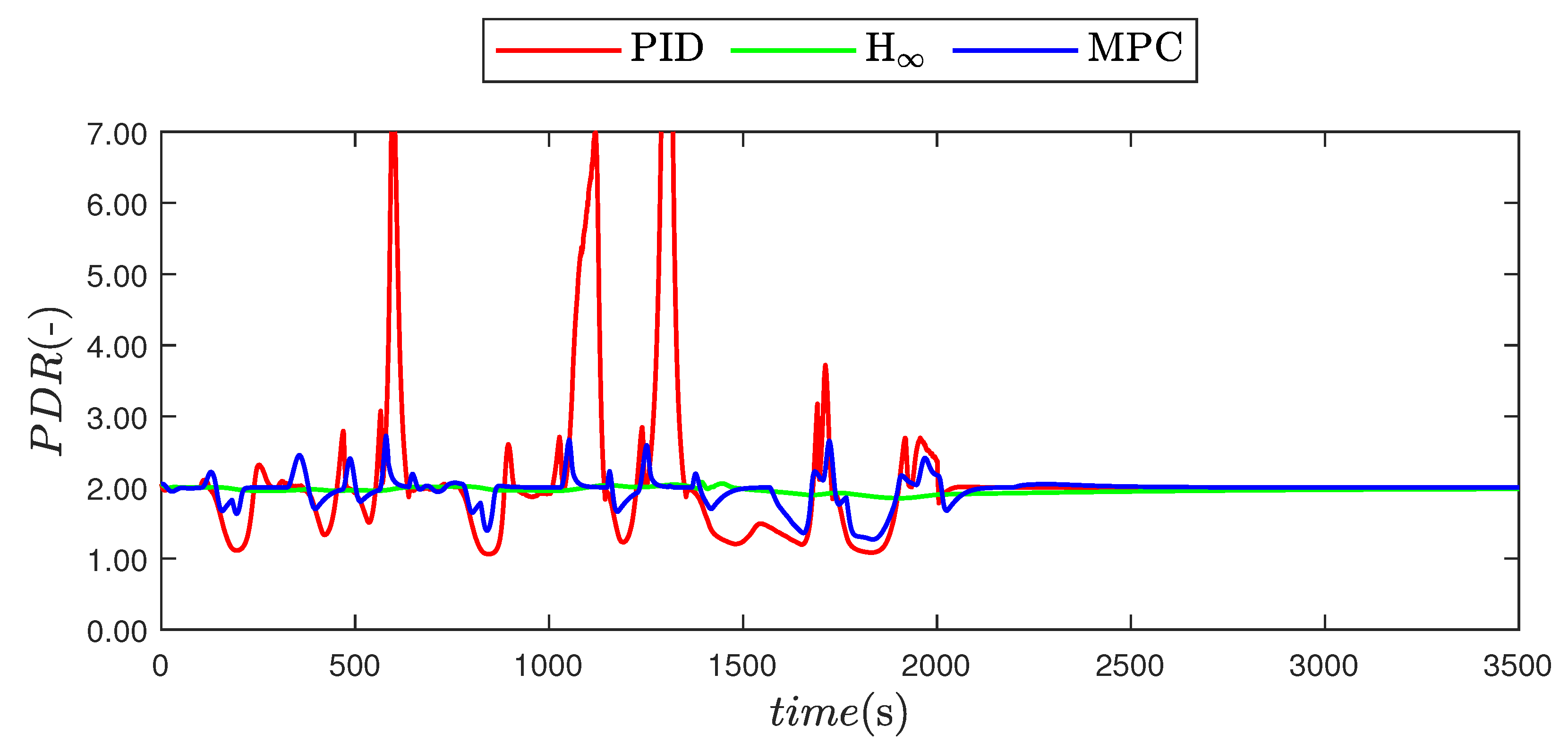
- The set-point for liquid interface height is 0.15 m, and the set-point for the PDR is 2, as these are the equilibrium points of the linear model.
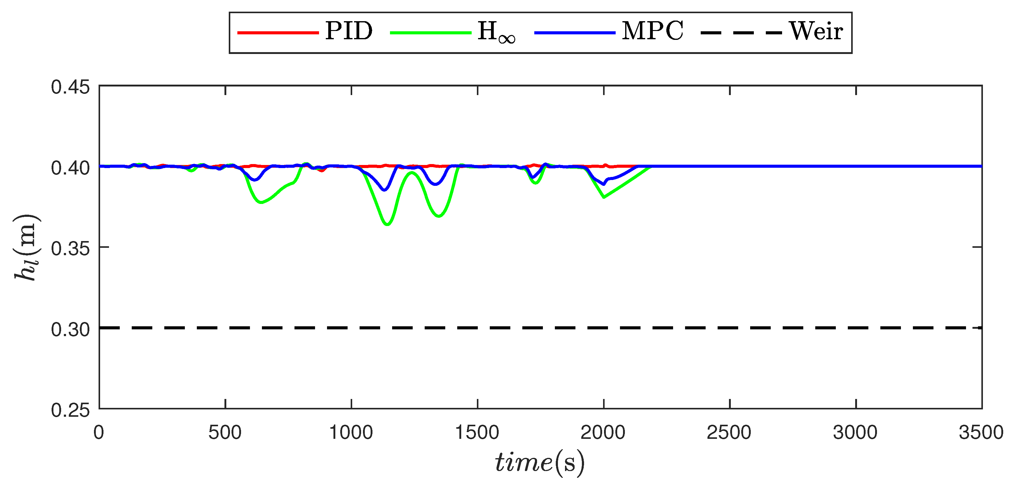
- The weir height is 0.3 m, and the set-point for total liquid height is 0.4 m, as these values keep above and below the weir at all times in the simulations, which is necessary due to model limitations.
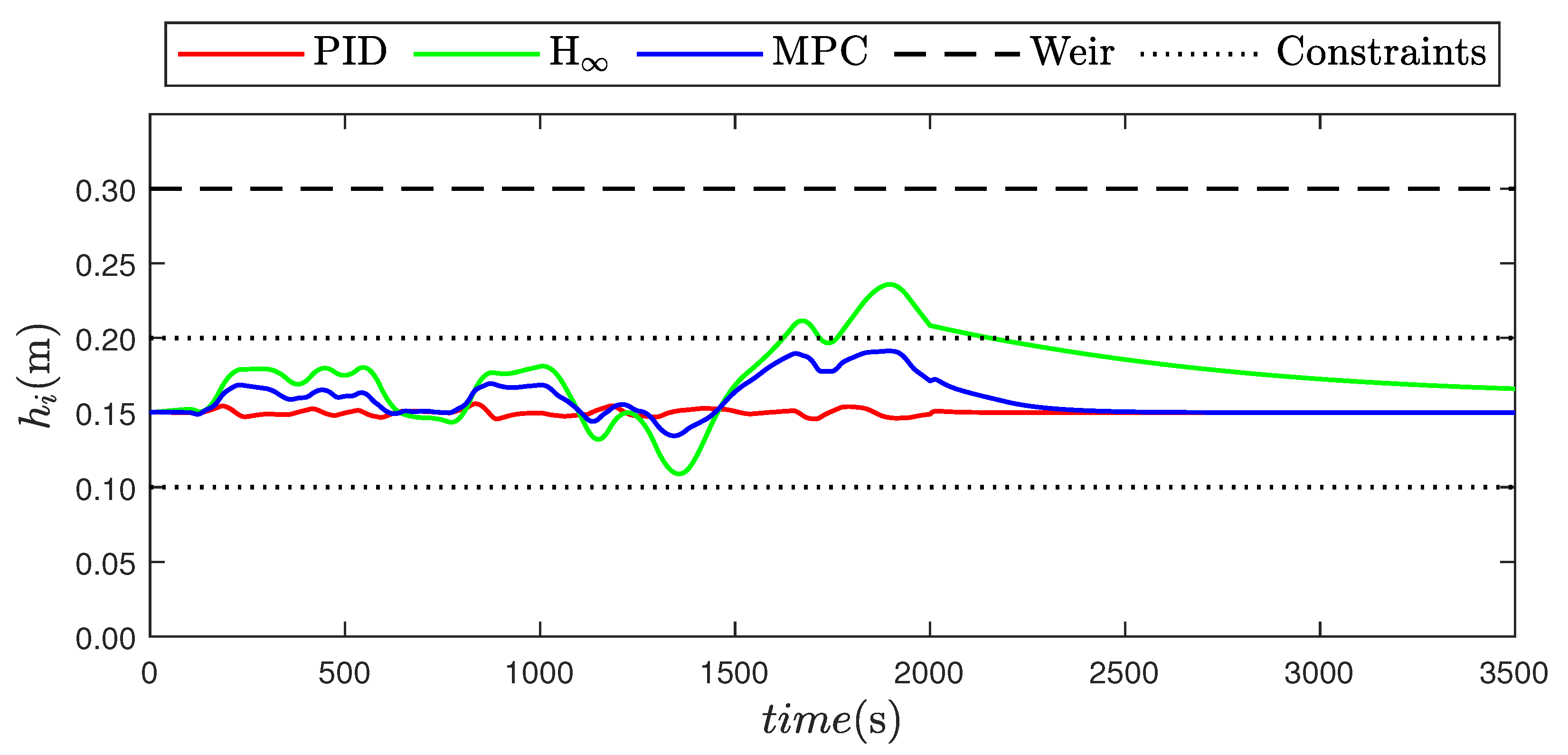
3. Results
4. Discussion
- Oil droplet breakup and coalescence, which are expected to decrease the separation performance at high flow rates, as increased shear force increases droplet breakup.
- Turbulence induced random walk, which causes the grade efficiency curve to asymptotically approach 100% rather than approaching 100% quadratically, as a function of droplet size.
- Dynamic flow fields, which attributes setting time for the flow fields rather than instantaneously occurring. This effect is expected to decrease the performance of the hydrocyclone as it is known for performing poorly during transient and varying input flow conditions [41].
Controller Performance
5. Conclusions
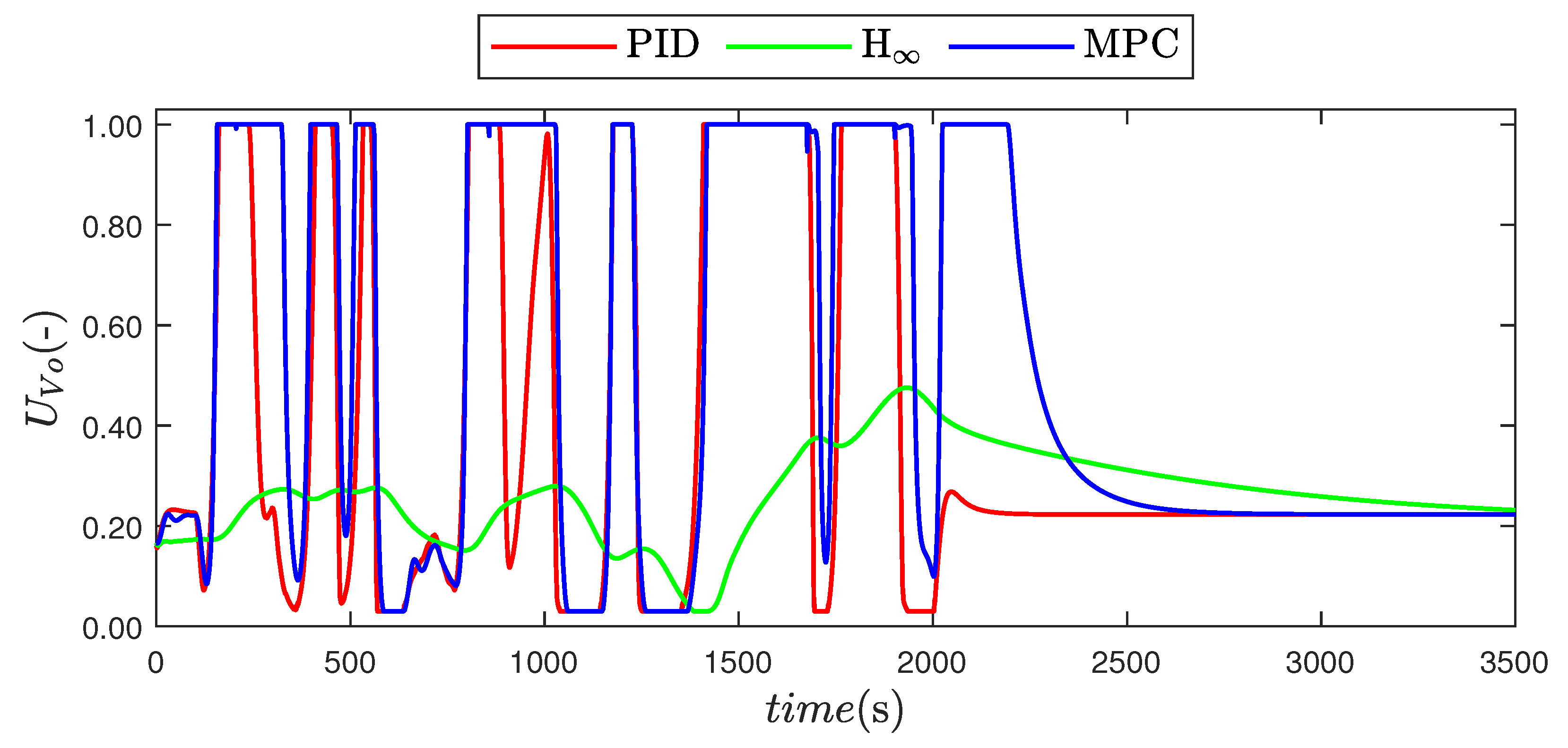
- The PID solution has the highest total valve distance traveled, which causes the most wear to the underflow and overflow valve.
- has the least total valve distance traveled.
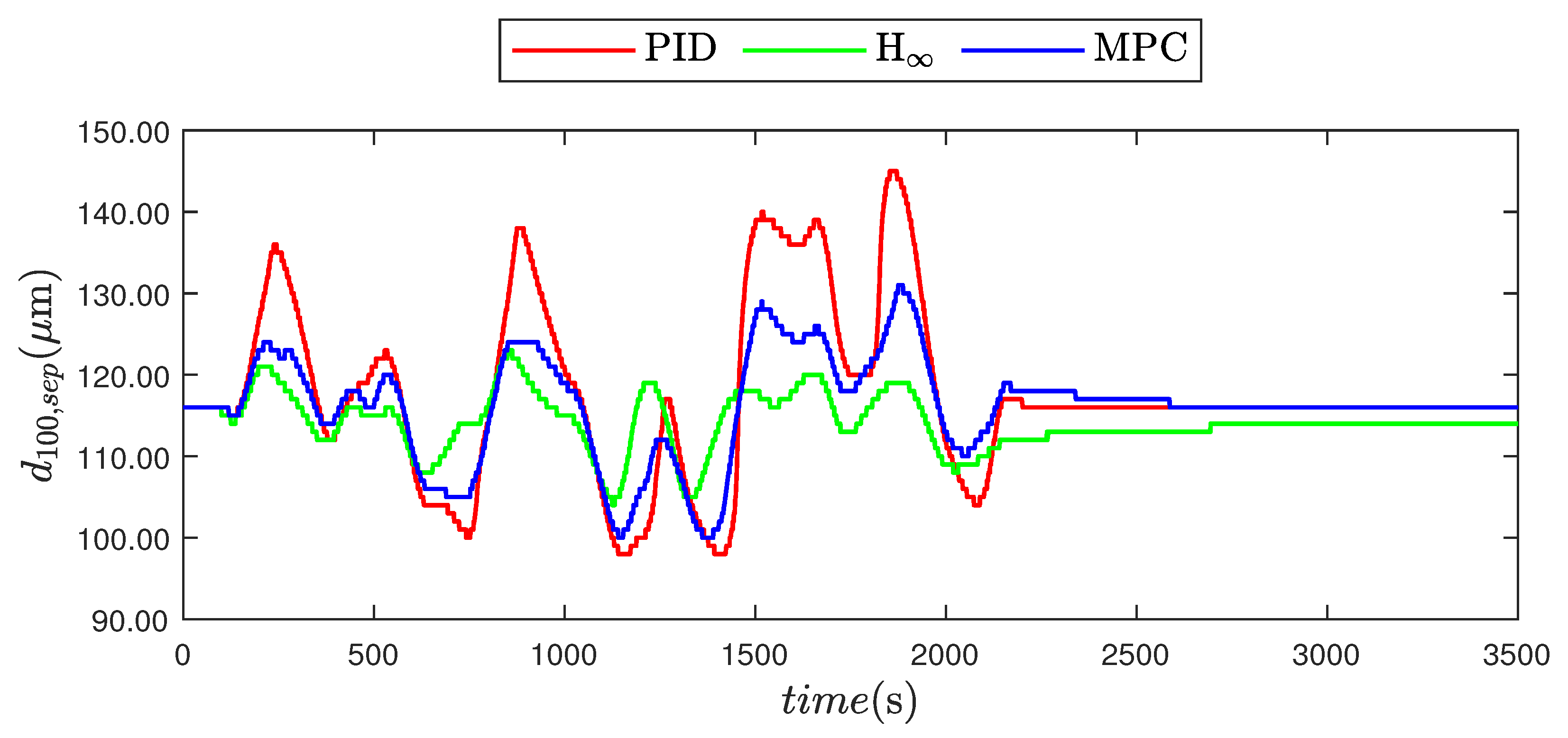
- Both PID and MPC solutions can keep between the chosen constraints, while the can not.
- Both MPC and solutions can avoid extreme PDR values, with keeping the most constant value.
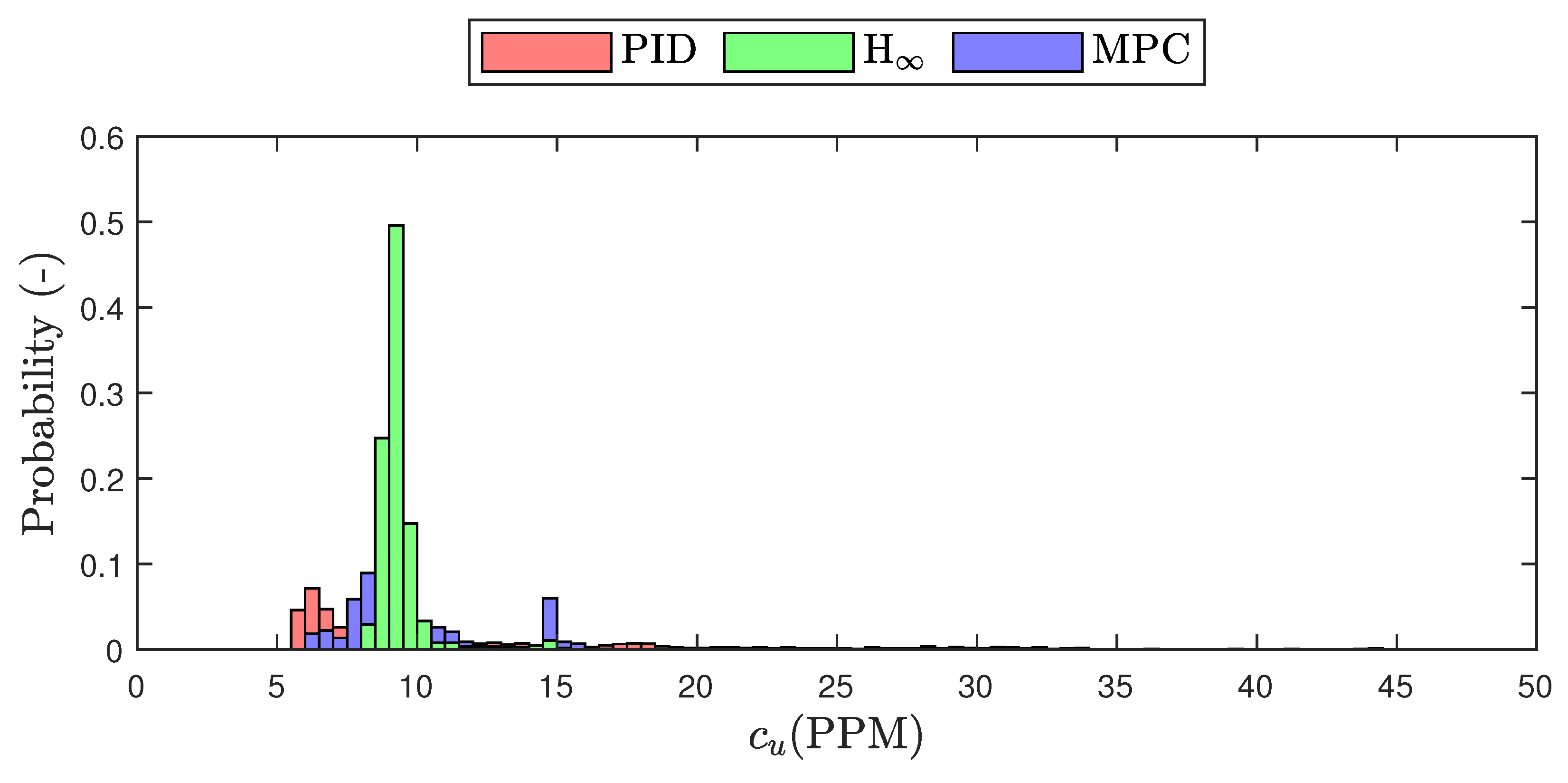
- PID control has the lowest mean (volumetric) but also the highest variance, resulting in the highest maximum concentration.
- Measured in mean (volumetric) the three solutions performs very similarly.
- Most of the performance metrics of MPC are between those of the PID and control.
- MPC is able to assign priority to manipulate interface level if a constraint is reached within the current sample’s prediction horizon.
Author Contributions
Funding
Data Availability Statement
Acknowledgments
Conflicts of Interest
Nomenclature
| Separator water cut in liquid inflow | |
| Hydrocyclone cone angle | |
| Density difference between water and oil | |
| Pressure difference | |
| Pressure difference over the overflow valve | |
| Pressure difference over the underflow valve | |
| Oil distribution vector at hydrocyclone underflow | |
| Approximated probability mass function of | |
| Oil distribution vector at separator water phase inlet | |
| Oil distribution vector at separator water outlet | |
| Separator liquid flow split | |
| Dynamic viscosity of water | |
| Continues oil distribution at separator water phase inlet | |
| Separator initial OiW ratio | |
| Separator initial WiO ratio | |
| Vector of droplet volumes | |
| Coefficients for Y, | |
| Separator final OiW ratio | |
| Separator final WiO ratio | |
| Function for the cross-section area of the separator below the height x | |
| Linear model state matrix | |
| Linear model disturbance input matrix | |
| Linear model control input matrix | |
| Hydrocyclone inlet speed imperfection coefficient | |
| Hydrocyclone tangential speed dropoff coefficient | |
| Linear model output matrix | |
| Upper output constraint for the MPC solution | |
| Lower output constraint for the MPC solution | |
| OiW concentration in hydrocyclone underflow | |
| OiW concentration in separator water outlet | |
| d | Vector of droplet sizes |
| Oil droplet diameter with 100% chance of being separated in the hydrocyclone | |
| Oil droplet diameter with 100% chance of being separated in the separator | |
| Oil droplet diameter with 50% chance of being separated in the hydrocyclone | |
| Oil droplet diameter with 50% chance of being separated in the separator | |
| Characteristic hydrocyclone diameters, | |
| Upper input constraint for the MPC solution | |
| Lower input constraint for the MPC solution | |
| Tracking error for control | |
| Tracking error for control | |
| Hammerstein function for the MPC solution | |
| Hydrocyclone flow split | |
| g | Gravitational acceleration |
| Separator liquid interface level | |
| Separator total liquid level | |
| Vertical traveled distance in the separator for each droplet size | |
| Cost function for the MPC solution |
| K | Flow conductance parameter |
| Dynamic controller for the solution | |
| Overflow valve flow conductance parameter | |
| Underflow valve flow conductance parameter | |
| Hydrocyclone segment axial lengths, | |
| Molar mass of the gas phase | |
| N | Possible solutions for |
| n | Hydrocyclone forced/frex coefficient |
| Separator residence time in terms of number of samples | |
| Augmented plant model for the solution | |
| Separator gas pressure | |
| Hydrocyclone pressure drop ration | |
| Q | Flow rate |
| Separator gas inflow rate | |
| Separator gas outflow rate | |
| Separator liquid inflow rate | |
| Separator oil outlet liquid flow rate | |
| Hydrocyclone overflow liquid flow rate | |
| Hydrocyclone underflow oil flow rate | |
| Hydrocyclone underflow liquid flow rate | |
| Separator water outlet liquid flow rate | |
| Separator water phase liquid flow rate | |
| R | Gas constant |
| Radial and axial coordinates inside the hydrocyclone | |
| Vector of all radial starting position of all critical oil droplet trajectories inside | |
| the hydrocyclone | |
| Set-point for control | |
| Radius of locus of zero axial velocity inside the hydrocyclone | |
| Set-point for control | |
| Recirculation rate | |
| The ratio of droplets remaining in the underflow | |
| The ratio of droplets remaining in the separator water outlet | |
| Inner hydocyclone wall radius as function of z | |
| Combined model sampling time | |
| T | Process temperature |
| Hydrocyclone dispersed phase tangential velocity field | |
| Separator residence time | |
| Incremental control inputs for the MPC solution | |
| Hydrocyclone dispersed phase radial velocity field | |
| Controllable inputs for the solution | |
| Controllable inputs for the MPC solution | |
| Unknown disturbance input for the MPC solution | |
| Overflow valve actuator set-point | |
| Underflow valve actuator set-point | |
| V | Output weight matrix for the MPC solution |
| Overflow valve position | |
| Superficial velocity through separator the water phase | |
| Terminal output weight matrix for the MPC solution | |
| Underflow valve position | |
| W | Input weight matrix for the MPC solution |
| Hydrocyclone dispersed phase axial velocity field | |
| Unknown disturbance input for the solution | |
| Estimated states for the MPC solution | |
| Y | Hydrocyclone axial velocity profile |
| Measured outputs for the solution | |
| Predicted outputs for the MPC solution | |
| Controlled outputs for the solution |
References
- Hansen, D. Online Monitoring and Analysis of Water Quality in Offshore Oil & Gas Production. Ph.D. Thesis, Aalborg Universitetsforlag, Aalborg, Denmark, 2020. [Google Scholar] [CrossRef]
- Administration, U.E.I. International Energy Outlook 2019. 2019. Available online: https://www.eia.gov/ (accessed on 19 December 2021).
- Choi, M. Hydrocyclone Produced Water Treatment for Offshore Developments. In SPE Annual Technical Conference and Exhibition; Society of Petroleum Engineers: New Orleans, LA, USA, 1990; pp. 473–480. [Google Scholar] [CrossRef]
- Amini, S.; Mowla, D.; Golkar, M.; Esmaeilzadeh, F. Mathematical modelling of a hydrocyclone for the down-hole oil-water separation (DOWS). Chem. Eng. Res. Des. 2012, 90, 2186–2195. [Google Scholar] [CrossRef]
- Produced Water Treatment: Yesterday, Today, and Tomorrow. Oil Gas Facil. 2012, 1. Available online: https://jpt.spe.org/produced-water-treatment-yesterday-today-and-tomorrow (accessed on 5 November 2021).
- Yang, Z.; Pedersen, S.; Løhndorf, P. Cleaning the Produced Water in Offshore Oil Production by Using Plant-wide Optimal Control Strategy. In Proceedings of the OCEANS’14 MTS/IEEE Conference, St. John’s, NL, Canada, 14–19 September 2014. [Google Scholar] [CrossRef]
- Yang, Z.; Pedersen, S.; Løhndorf, P.; Mai, C.; Hansen, L.; Jepsen, K.; Aillos, A.; Andreasen, A. Plant-wide Control Strategy for Improving Produced Water Treatment. In Proceedings of the 2016 International Field Exploration and Development Conference (IFEDC), Beijing, China, 11–12 August 2016. [Google Scholar] [CrossRef]
- Fakhru’l-Razi, A.; Pendashteh, A.; Abdullah, L.C.; Biak, D.R.A.; Madaeni, S.S.; Abidin, Z.Z. Review of technologies for oil and gas produced water treatment. J. Hazard. Mater. 2009, 170, 530–551. [Google Scholar] [CrossRef]
- OSPAR Commission. North Sea Manual on Maritime Oil Pollution Offences; Technical Report; OSPAR Commission: London, UK, 2010. [Google Scholar]
- Danish Environmental Protection Agency. Generel Tilladelse for Mærsk Olie og Gas A/S (Mærsk Olie) til Anvendelse, Udledning og Anden Bortskaffelse af Stoffer og Materialer, Herunder Olie og Kemikalier i Produktions- og Injektionsvand fra Produktionsenhederne Halfdan, Dan, Tyra og Gorm for Perio; Technical Report; Danish Environmental Protection Agency: Copenhagen, Denmark, 2016. [Google Scholar]
- Brette, F.; Machado, B.; Cros, C.; Incardona, J.P.; Scholz, N.L.; Block, B.A. Crude oil impairs cardiac excitation-contraction coupling in fish. Science 2014, 343, 772–776. [Google Scholar] [CrossRef]
- Ekins, P.; Vanner, R.; Firebrace, J. Zero emissions of oil in water from offshore oil and gas installations: Economic and environmental implications. J. Clean. Prod. 2007, 15, 1302–1315. [Google Scholar] [CrossRef]
- Bakke, T.; Klungsøyr, J.; Sanni, S. Environmental impacts of produced water and drilling waste discharges from the Norwegian offshore petroleum industry. Mar. Environ. Res. 2013, 92, 154–169. [Google Scholar] [CrossRef] [Green Version]
- Hasselberg, L.; Meier, S.; Svardal, A. Effects of alkylphenols on redox status in first spawning Atlantic cod (Gadus morhua). Aquat. Toxicol. 2004, 69, 95–105. [Google Scholar] [CrossRef]
- Hylland, K. Polycyclic Aromatic Hydrocarbon (PAH) Ecotoxicology in Marine Ecosystems. J. Toxicol. Environ. Health Part A 2007, 69, 109–123. [Google Scholar] [CrossRef] [PubMed]
- Thomas, K.V.; Langford, K.; Petersen, K.; Smith, A.J.; Tollefsen, K.E. Effect-Directed Identification of Naphthenic Acids as Important in Vitro Xeno-Estrogens and Anti-Androgens in North Sea Offshore Produced Water Discharges. Environ. Sci. Technol. 2009, 43, 8066–8071. [Google Scholar] [CrossRef] [PubMed]
- Yang, M. Measurement of Oil in Produced Water. In Produced Water, 1st ed.; Lee, K., Neff, J.M., Eds.; Springer: New York, NY, USA, 2011. [Google Scholar] [CrossRef]
- Toril Inga, R.; Garpestad, E.; Tangvald, M.; Frost, T. Results and Commitments from the Zero Discharge Work on Produced Water Discharges on the Norwegian Continental Shelf. In Proceedings of SPE International Conference on Health, Safety, and Environment in Oil and Gas Exploration and Production; Society of Petroleum Engineers: Calgary, AB, Canada, 2004; pp. 1327–1332. [Google Scholar] [CrossRef]
- Bram, M.V. Greybox Modeling and Validation of Deoiling Hydrocyclones. Ph.D. Thesis, Aalborg Universitetsforlag, Aalborg, Denmark, 2020. [Google Scholar]
- Husveg, T.; Johansen, O.; Bilstad, T. Operational control of hydrocyclones during variable produced water flow rates—Frøy case study. SPE Prod. Oper. 2007, 22, 294–300. [Google Scholar] [CrossRef]
- Løhndorf, P.; Pedersen, S.; Yang, Z. Challenges in Modelling and Control of Offshore De-oiling Hydrocyclone Systems. In Proceedings of the 13th EuropeanWorkshop on Advanced Control & Diagnosis, ACD’16, Lille, France, 17–18 November 2016; IOP Publishing: Bristol, UK, 2017; Volume 783. [Google Scholar] [CrossRef]
- Bram, M.V.; Hassan, A.A.; Hansen, D.S.; Durdevic, P.; Pedersen, S.; Yang, Z. Experimental modeling of a deoiling hydrocyclone system. In Proceedings of the 2015 20th International Conference on Methods and Models in Automation and Robotics (MMAR), Miedzyzdroje, Poland, 24–27 August 2015; pp. 1080–1085. [Google Scholar]
- Mokhatab, S.; Towler, B.F. Severe Slugging in Flexible Risers: Review of Experimental Investigations and OLGA Predictions. Pet. Sci. Technol. 2007, 25, 867–880. [Google Scholar] [CrossRef]
- Pedersen, S.; Durdevic, P.; Yang, Z. Challenges in slug modeling and control for offshore oil and gas productions: A review study. Int. J. Multiph. Flow 2017, 88, 270–284. [Google Scholar] [CrossRef]
- Mokhatab, S. Severe Slugging in Offshore Production Systems; Nova Science Publishers: Hauppauge, NY, USA, 2010. [Google Scholar]
- Pedersen, S.; Løhndorf, P.; Yang, Z. Influence of riser-induced slugs on the downstream separation processes. J. Pet. Sci. Eng. 2017, 154, 337–343. [Google Scholar] [CrossRef]
- Pedersen, S. Plant-Wide Anti-Slug Control for Offshore Oil and Gas Processes. Ph.D. Thesis, Aalborg Universitetsforlag, Aalborg, Denmark, 2016. [Google Scholar] [CrossRef]
- Durdevic, P.; Yang, Z. Application of H∞ Robust Control on a Scaled Offshore Oil and Gas De-oiling Facility. Energies 2018, 11, 287. [Google Scholar] [CrossRef] [Green Version]
- Hansen, L.; Durdevic, P.; Jepsen, K.L.; Yang, Z. Plant-wide Optimal Control of an Offshore De-oiling Process Using MPC Technique. IFAC-PapersOnLine 2018, 51, 144–150. [Google Scholar] [CrossRef]
- Das, T.; Heggheim, S.J.; Dudek, M.; Verheyleweghen, A.; Jäschke, J. Optimal Operation of a Subsea Separation System Including a Coalescence Based Gravity Separator Model and a Produced Water Treatment Section. Ind. Eng. Chem. Res. 2019, 58, 4168–4185. [Google Scholar] [CrossRef]
- Hansen, L.; Jepsen, K.L.; Durdevic, P.; Yang, Z. Comparison of Inlet Observers for a De-Oiling Gravity Separator. In 15th European Workshop on Advanced Control and Diagnosis (ACD 2019); Springer International Publishing AG: Basel, Switzerland, 2022. [Google Scholar] [CrossRef]
- Bram, M.V.; Jespersen, S.; Hansen, D.S.; Yang, Z. Control-Oriented Modeling and Experimental Validation of a Deoiling Hydrocyclone System. Processes 2020, 8, 1010. [Google Scholar] [CrossRef]
- Pedersen, S.; Bram, M.V. The Impact of Riser-Induced Slugs on the Downstream Deoiling Efficiency. J. Mar. Sci. Eng. 2021, 9, 391. [Google Scholar] [CrossRef]
- Bram, M.V.; Hansen, L.; Hansen, D.S.; Yang, Z. Grey-Box modeling of an offshore deoiling hydrocyclone system. In Proceedings of the 2017 IEEE Conference on Control Technology and Applications (CCTA), Maui, HI, USA, 27–30 August 2017; IEEE: Manhattan, NY, USA, 2017; pp. 94–98. [Google Scholar] [CrossRef]
- Wolbert, D.; Ma, B.F.; Aurelle, Y.; Seureau, J. Efficiency estimation of liquid–liquid Hydrocyclones using trajectory analysis. AIChE J. 1995, 41, 1395–1402. [Google Scholar] [CrossRef]
- Bram, M.V.; Hansen, L.; Hansen, D.S.; Yang, Z. Hydrocyclone Separation Efficiency Modeled by Flow Resistances and Droplet Trajectories. IFAC-PapersOnLine 2018, 51, 132–137. [Google Scholar] [CrossRef]
- Bram, M.V.; Hansen, L.; Hansen, D.S.; Yang, Z. Extended Grey-Box Modeling of Real-Time Hydrocyclone Separation Efficiency. In Proceedings of the 2019 18th European Control Conference (ECC), Naples, Italy, 25–28 June 2019; IEEE: Manhattan, NY, USA, 2019; pp. 3625–3631. [Google Scholar] [CrossRef]
- The Danish Energy Agency. Yearly Production, Injection, Flare, Fuel and Export in Si Units 1972–2017; The Danish Energy Agency: Copenhagen, Denmark, 2018. [Google Scholar]
- Thew, M. Hydrocyclone Redesign for Liquid-Liquid Separation. Chem. Eng. 1986, 427, 17–23. [Google Scholar]
- Meldrum, N. Hydrocyclones: A Solutlon to Produced-Water Treatment. SPE Prod. Eng. 1988, 3, 669–676. [Google Scholar] [CrossRef]
- Husveg, T.; Rambeau, O.; Drengstig, T.; Bilstad, T. Performance of a deoiling hydrocyclone during variable flow rates. Miner. Eng. 2007, 20, 368–379. [Google Scholar] [CrossRef]
- Bortoff, S.A.; Schwerdtner, P.; Danielson, C.; Di Cairano, S. H-Infinity Loop-Shaped Model Predictive Control with Heat Pump Application. In Proceedings of the 2019 18th European Control Conference (ECC), Naples, Italy, 25–28 June 2019; IEEE: Manhattan, NY, USA, 2019; pp. 2386–2393. [Google Scholar] [CrossRef]


| Total Accumulated | Unit | PID | MPC | ||
|---|---|---|---|---|---|
| Liquid flow separator inlet | (L) | 1785.7 | 1785.7 | 1785.7 | |
| Liquid flow separator oil outlet | (L) | 355.55 | 364.06 | 355.58 | |
| Liquid flow separator water outlet | (L) | 1430.1 | 1421.6 | 1430.1 | |
| Oil flow separator water outlet | (mL) | 1588.3 | 1497.4 | 1551.4 | |
| Liquid flow hydrocyclone overflow | (L) | 93.071 | 101.85 | 101.06 | |
| Liquid flow hydrocyclone underflow | (L) | 1337.1 | 1319.8 | 1329 | |
| Oil flow hydrocyclone underflow | (mL) | 12.190 | 12.241 | 12.215 | |
| Underflow valve travel distance | (-) | 7.5994 | 0.42053 | 3.6072 | |
| Overflow valve travel distance | (-) | 16.143 | 1.4416 | 15.147 | |
| Volume Average | |||||
| Oil concentration separator water outlet | (PPM) | 1110.6 | 1053.3 | 1084.9 | |
| Oil concentration hydrocyclone underflow | (PPM) | 9.1174 | 9.2755 | 9.191 | |
| Time Sample Average | |||||
| mean | (PPM) | 1095.9 | 1052.8 | 1077.9 | |
| Oil concentration separator water outlet | std | (PPM) | 131.1 | 43.874 | 79.064 |
| max | (PPM) | 1454 | 1162.7 | 1273.2 | |
| mean | (PPM) | 10.426 | 9.3391 | 9.4758 | |
| Oil concentration hydrocyclone underflow | std | (PPM) | 5.2978 | 0.93424 | 1.9029 |
| max | (PPM) | 44.814 | 15.206 | 16.823 |
| Metric | PID | MPC | |
|---|---|---|---|
| Control system complexity | Low | Medium | High |
| Total oil discharge | Similar | Similar | Similar |
| Discharge concentration variation | High | Low | Medium |
| Valve wear | High | Low | Medium |
| Disturbance propagation | High | Low | Medium |
| Explicitly defined constraints | No | No | Yes |
Publisher’s Note: MDPI stays neutral with regard to jurisdictional claims in published maps and institutional affiliations. |
© 2022 by the authors. Licensee MDPI, Basel, Switzerland. This article is an open access article distributed under the terms and conditions of the Creative Commons Attribution (CC BY) license (https://creativecommons.org/licenses/by/4.0/).
Share and Cite
Hansen, L.; Bram, M.V.; Pedersen, S.; Yang, Z. Performance Comparison of Control Strategies for Plant-Wide Produced Water Treatment. Energies 2022, 15, 418. https://doi.org/10.3390/en15020418
Hansen L, Bram MV, Pedersen S, Yang Z. Performance Comparison of Control Strategies for Plant-Wide Produced Water Treatment. Energies. 2022; 15(2):418. https://doi.org/10.3390/en15020418
Chicago/Turabian StyleHansen, Leif, Mads Valentin Bram, Simon Pedersen, and Zhenyu Yang. 2022. "Performance Comparison of Control Strategies for Plant-Wide Produced Water Treatment" Energies 15, no. 2: 418. https://doi.org/10.3390/en15020418