Abstract
Induction motors are widely used in industry and are essential to industrial processes. The faults in motors lead to high repair costs and cause financial losses resulting from unexpected downtime. Early detection of faults in induction motors has become necessary and critical in reducing costs. Most motor faults are caused by bearing failure. Machine learning-based diagnostic methods are proposed in this study. These methods use effective features. First, load currents of healthy and faulty motors are measured while the rotating speed is changing continuously. Second, experiments revealed the relationship between the magnitude of the amplitude of specific signals and the rotating speed, and the rotating speed is treated as a new feature. Third, machine learning-based diagnoses are conducted. Finally, the effectiveness of machine learning-based diagnostic methods is verified using experimental data.
1. Introduction
Induction motors play a significant role because of their robustness, low cost, and efficiency. Thus, successive and unconscious use of a motor with a minor fault can lead to catastrophic faults and unexpected standstill. To reduce costs by avoiding an emergency shutdown, for example, in a production line, fault detection in induction motors in an initial stage has become necessary and critical.
According to an IEEE (Institute of Electrical and Electronics Engineers) motor reliability study for large motors above 200 hp, bearing faults are the most common single cause of motor failure (41%), followed by stator faults (37%), ad and rotor faults (10%) [1]. Though a critical element in induction motors is bearing, approximately 40% of motor damages occur in it. Unexpected breakdown can be avoided by detecting faults at an early stage.
Several studies are being conducted to investigate the detection of bearing faults. The most common detection method used in [2,3,4,5] has some disadvantages such as the high cost of vibration sensors and installation requirements. Acoustic emission-based techniques are used to diagnose bearing faults [6,7,8]. Furthermore, multi-physical fiber optic sensors for bearing condition monitoring [9], and a driving sound-based technique for diagnosing bearing and short-circuit faults [10] are proposed.
Among the several methods, motor current signature analysis (MCSA) has been commonly used, showing satisfactory performance for diagnosing diverse bearing failures [11,12,13,14,15,16,17]. MCSA has several advantages, including that it is non-invasive and does not require special sensors. The analysis can be performed online; thus, enabling the identification of several types of faults.
Though there are several advantages of MCSA, such as economic savings and simple implementation, it suffers from several practical issues. For example, the magnitude of stator currents at bearing fault signature frequencies can vary depending on the load and rotating speed, making it difficult to identify threshold values of the stator current to trigger the fault alarm at a certain operating condition [15]. According to [18], an increase in load current can cause fault misdetection. Therefore, thorough and systematic testing is required when the bearing is under a healthy state, and these healthy data must be gathered and classified at different load conditions.
To address this issue, researchers previously proposed a Support Vector Machine (SVM)-based diagnostic method using features extracted from the frequency spectrum of load current obtained at four constant rotating speeds [14]. The fault diagnosis was discussed under light load conditions. Experiments and diagnosis under heavy load conditions and the condition that the rotating speed changes continuously are required when operating motors at a site. The author in [15] proposed the method to diagnose the bearing fault using the current signals in the time domain. However, the proposed method was evaluated by using data obtained under no load and rated load. A model-based approach is proposed to quantify the bearing fault severity while the motor is running at any speed [17]. In this study, the indicator of the bearing fault is used based on the transfer function, which is the model of the motor. Generally, parameters in motors change because of the change in the internal temperature. In the case of applying the method at the site, it is necessary to conduct some experiments to determine the effect of the parameter change on the diagnosis accuracy through some experiments.
Deep learning-based methods for bearing fault diagnosis are proposed [16,19]. Generally, deep learning-based methods have a problem in that it often takes a lot more time for training than machine learning-based methods.
This paper proposes an on-line bearing fault diagnosis method based on the combination of selective features and machine learning. It involves the following novelty:
(1) Fault detection at its initial stage: The bearing fault target is a hole of 0.5 mm in diameter, which is smaller than the reported holes ranging from 3.0 to 1.0 mm [20,21,22,23]. Fault detection at its initial stage may enable to track progression of the fault and give important information of repair and/or replacement.
(2) Rotating speed as a new feature: Two features (amplitude of specific two frequency components in load current), which is proposed in our previous paper [14], is not enough to diagnose a small hole. Rotating speed of motor is selected as a new feature and added to the previous two features, which is proven to be effective in diagnosis.
(3) High performance diagnosis: The combination of the three selective features and machine learning achieves high diagnosis accuracy. Rotating speed is a powerful feature in diagnosis because a high accuracy rate is obtained regardless of the types of machine learning (Support Vector Machine, Random Forest, and Neural Network).
The present paper consists of the following four parts: First, the load currents of healthy and faulty motors are measured while the rotating speed is changing continuously. Second, two signals with specific frequencies are extracted, and experiments are performed to reveal the relationship between the magnitude of the amplitude of the signals and the rotating speed. Based on the results, the rotating speed is also considered a new feature. Third, machine learning-based diagnostic methods are used to improve diagnostic accuracy. Finally, the effectiveness of the proposed method is demonstrated using the experimental data.
2. Experiments
2.1. Experimental Setup
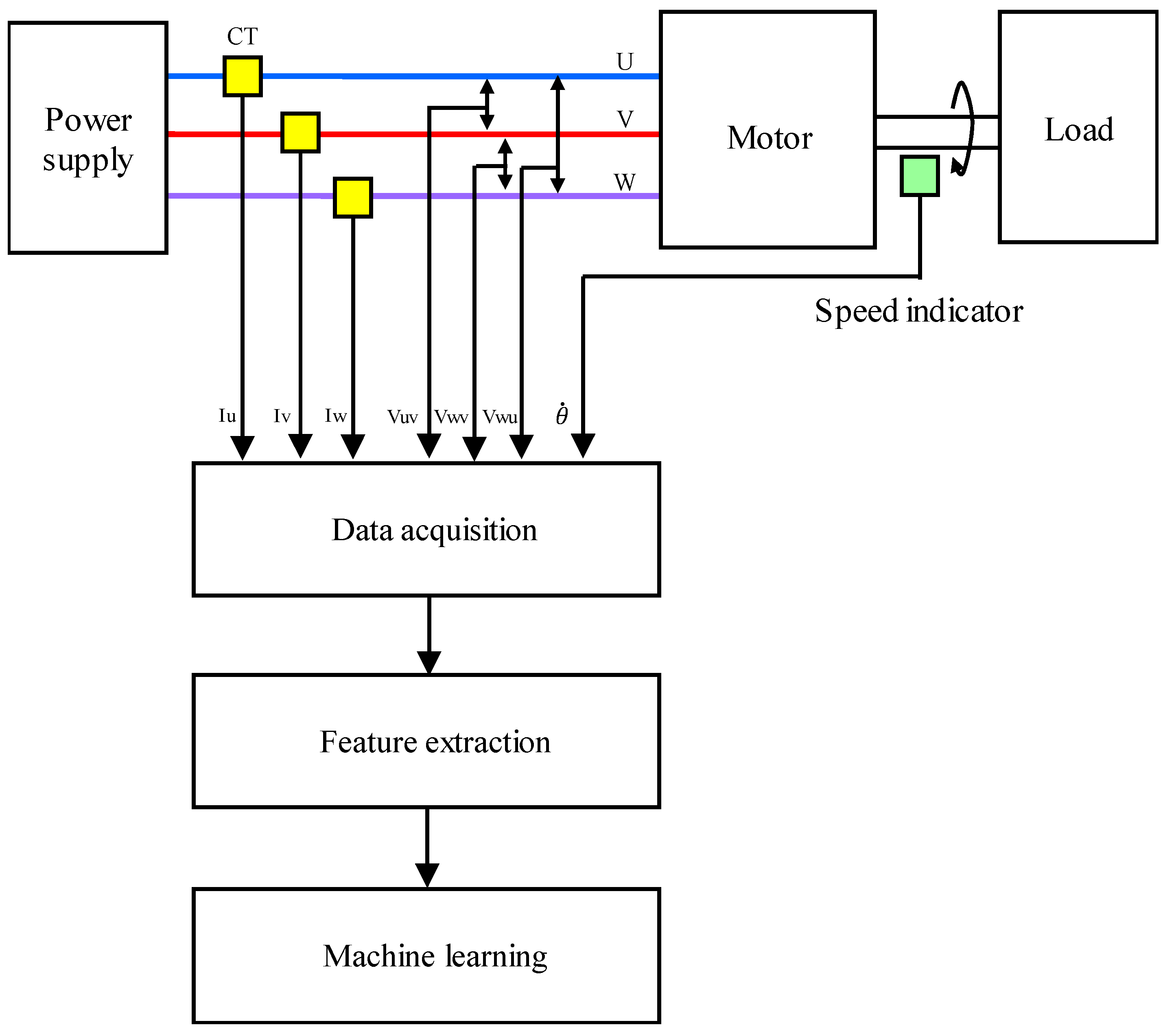
The experimental setup is shown in Figure 1. A three-phase induction motor (2.2 kW, 200 V, 8.5 A, 1740 min−1, 4 poles) was used as a specimen. The rotating speed was gradually changed between 1780 and 1730 min−1 by adjusting a load. The applied voltage ranged from 195 to 205 V. The power supply frequency was 60 Hz.

Figure 1.
Experimental setup.
Current probes (HIOKI 9695-02, Ueda, Japan), voltage probes (HIOKI 9666, Ueda, Japan), and speed indicator (ONOSOKKI HT-5500, Yokohama, Japan) were used for continuous monitoring of the load currents, line-to-line voltages, and the rotating speed, respectively. After undergoing A/D conversion, the output signals from these sensors were saved onto a recording medium in a note PC. The measurement equipment was developed by the authors, which enabled the current and voltage measurement up to 20 A and 300 V with a tolerance error of ±2%, respectively. The sampling time was set to 10 s, and the data recording length was 217 per channel. Data acquisition was triggered at 30 s intervals by a timer signal. Data transfer to the PC takes no more than 20 s.
After data collection, effective features for the bearing diagnosis are extracted. Using these features, a machine learning-based diagnostic method is used.
2.2. Reproduction of Faults
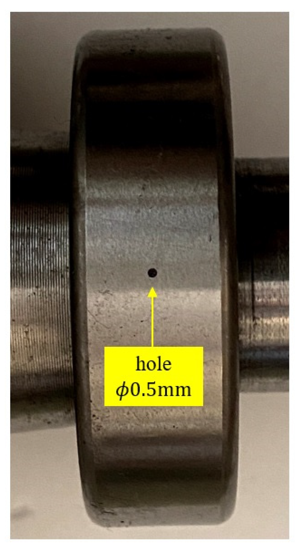
Because collecting motors with bearing faults from factories is a difficult and time-consuming task, a hole was artificially introduced to the surface of a bearing’s outer raceway (Figure 2). The diameter of the hole is 0.5 mm and the depth is 0.5 mm. The size was determined considering another objective: the development of a diagnostic method which can detect a fault as early as possible in its initial stage. The hole is small enough because the reported diameter of a hole ranges between 3.0 and 1.0 mm [20,21,22,23]. Healthy bearings were also used for reference.

Figure 2.
Production of bearing fault.
3. Analysis of Characteristics of Load Current
3.1. Frequency Spectrum of Load Current
Fast Fourier transform was performed using waveforms of the U-phase current obtained. The frequency resolution is 0.76 Hz. An example of a frequency spectrum of faulty and healthy bearings at a rotating speed of 1750 min−1 is shown in Figure 3. The amplitude of the figure is normalized so that the maximum is set to 0 dB. The difference in amplitude is recognized around 30 and 90 Hz between spectra of faulty and healthy bearings. A similar difference is also observed in spectra obtained at other rotating speeds because when a mechanical fault occurs in a rotor, such as bearing damage, and the rotor becomes unbalanced, the rotor fluctuates in the rotating frequency and the load current is subjected to amplitude modulation by the rotating frequency . Therefore, the sidebands of are generated around the load current frequency [24].
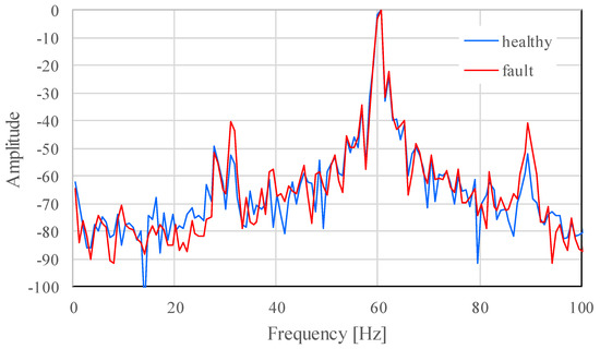
Figure 3.
Spectrum of current rotating at 1750 min−1.
3.2. Two-Dimensional Feature Distribution
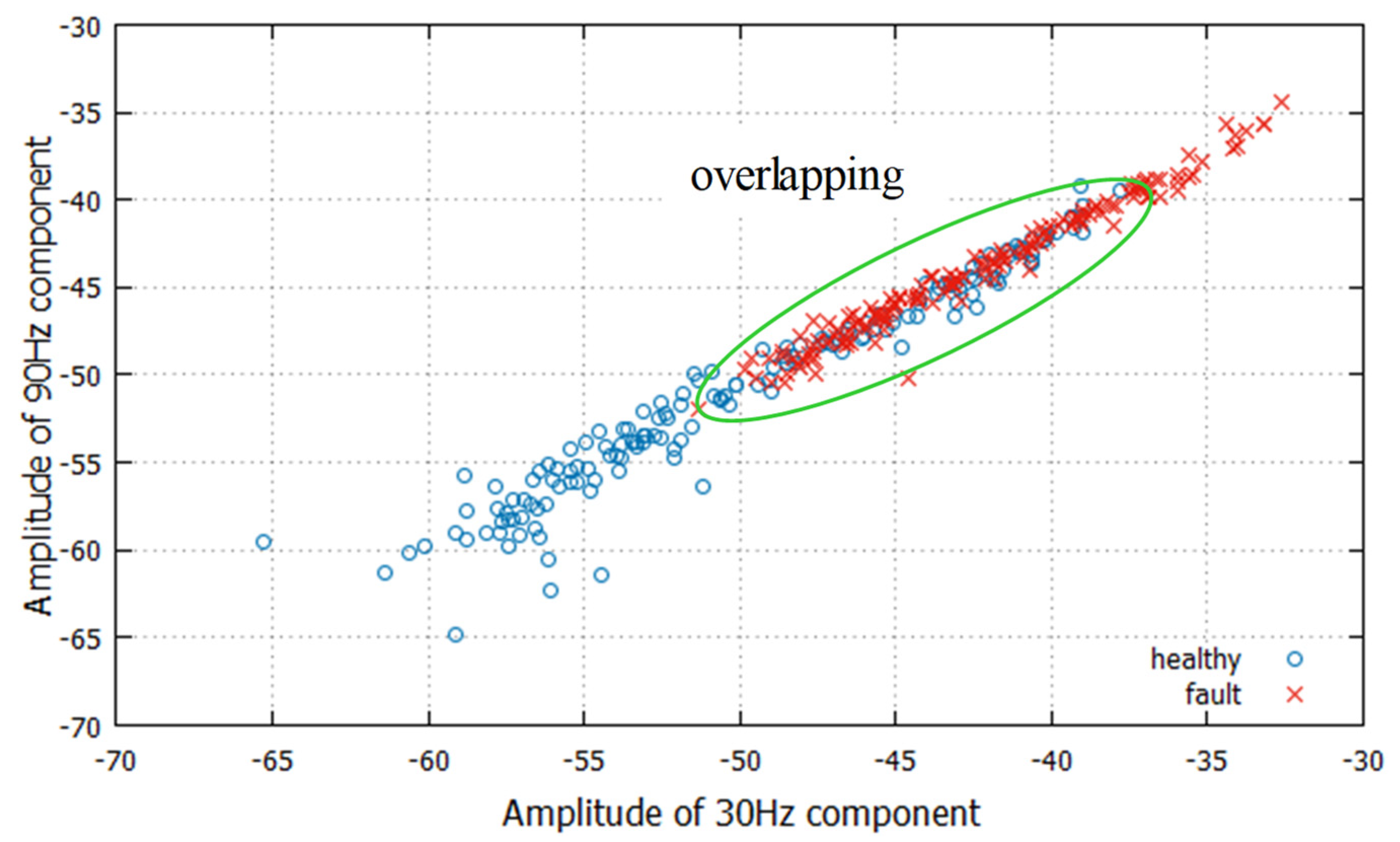
Figure 4 shows the feature distribution of healthy and faulty bearings, where the x- and y-axis represent the components of sidebands of the rotating frequency, respectively. From frequency spectra of the U-phase current, 140 data are obtained for each bearing condition (Figure 3). Depending on the bearing condition, features gather in a limited region. However, significant overlapping of two feature distributions occurs, which may affect the accuracy of diagnosis.
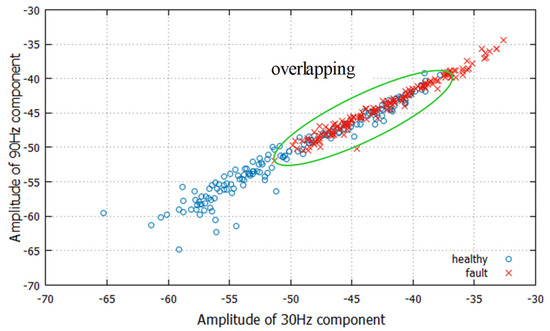
Figure 4.
Two-dimensional feature distribution.
3.3. Three-Dimensional Feature Distribution
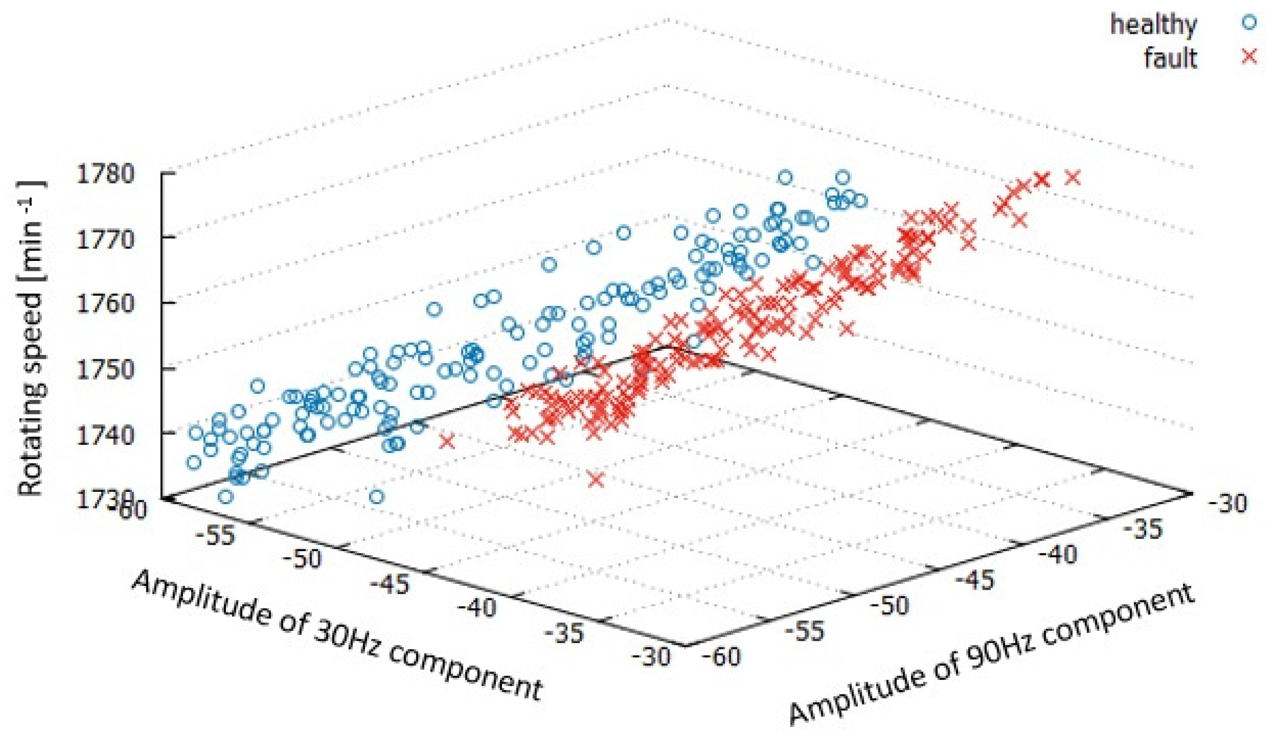
Figure 5 shows the rotating frequency dependence of the amplitude of the sidebands of around 30 and 90 Hz components. For each bearing condition, 160 data are shown. The amplitude of around 30 and 90 Hz components decreases almost linearly, decreasing the rotating speed regardless of the bearing condition. The data of faulty bearings are stored separately from the data from healthy bearings, with only a slight overlapping between them. Compared with Figure 4, the superiority of the three-dimensional display is obvious. The combination of three items (amplitude of the sidebands of the rotating frequency around 30 and 90 Hz components, and rotating speed) are promising for the bearing diagnosis when the rotating speed is changing constantly. Therefore, they are treated as fault diagnostics features in the improved diagnostics method. This is reasonable because the rotating speed may change at the site because of variations in load, fluctuation of voltage, and so on.

Figure 5.
Three-dimensional feature distribution.
4. Proposal of Improved Diagnostics Method
In this study, a machine learning-based diagnostic method is proposed using new features explained above. Here, three machine-learning algorithms; Support Vector Machine (SVM), Random Forest (RF), and Neural Network (NN) are used.
4.1. Fault Diagnosis Based on SVM
The concept is described briefly. SVM is a supervised machine-learning algorithm and is widely used as a promising tool [25,26,27].
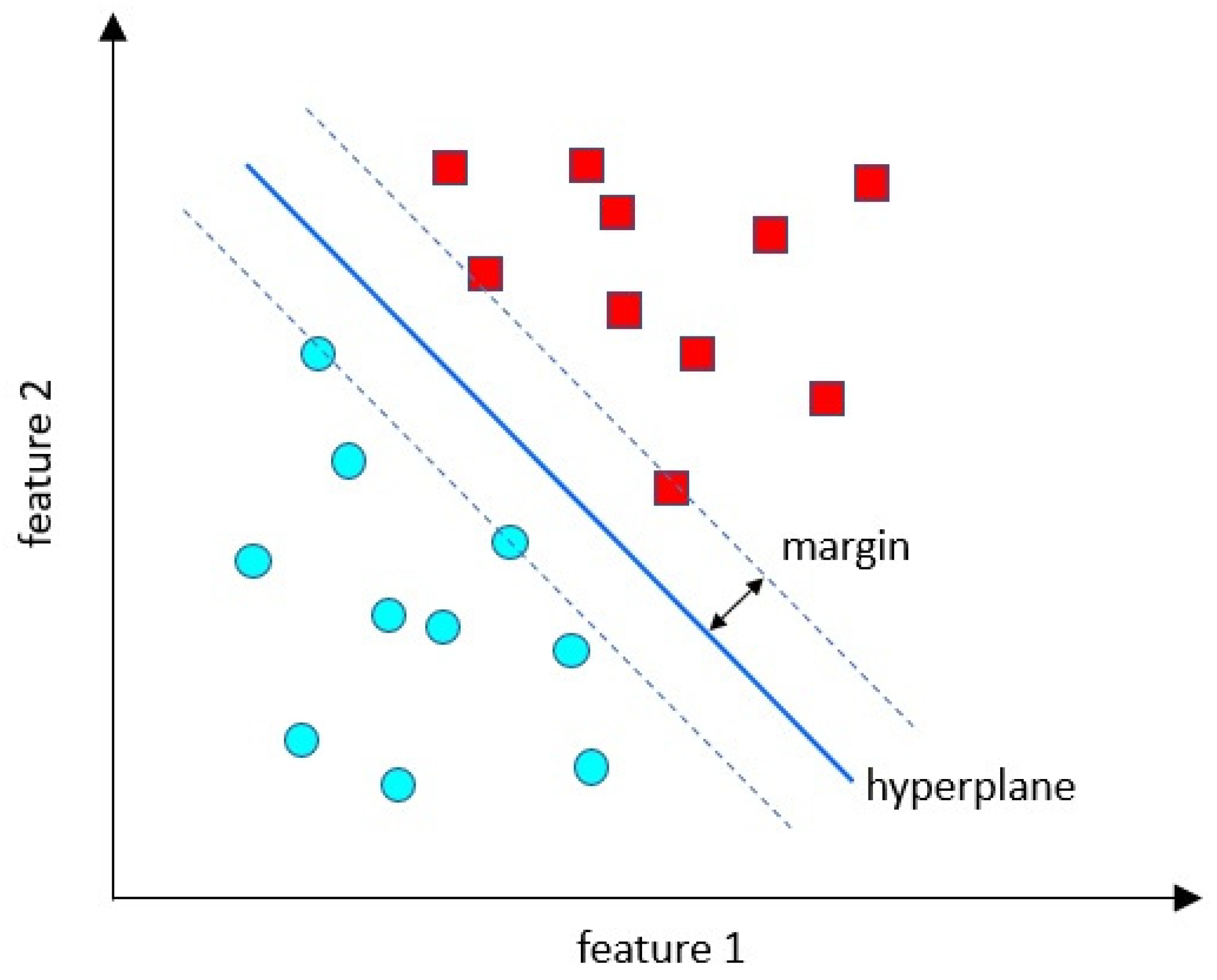
For example, data separated to two classes are distributed as shown in Figure 6. They are separated by the decision boundary. The purpose of the SVM algorithm is to find the decision boundary. The best boundary is called a hyperplane. The dimensions of the hyperplane depend on the features present in the dataset, which means that, if there are two features, then the hyperplane will be a straight line. Additionally, if there are three features, then the hyperplane will be a plane. The hyperplane is created so that it has a maximum margin, which means a maximum distance between the data points.
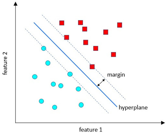
Figure 6.
Concept of SVM.
Data obtained in the experiment described in Section 2 were used to construct a diagnosis model. For healthy bearing (denoted as No. 1) or faulty bearing (No. 2), 100 data each were selected randomly. A datum consisted of three features: values of the sideband components around 30 and 90 Hz of load current spectrum, and rotating speed. The rotating speed ranged between 1780 and 1730 min−1.
In SVM, two parameters; gamma and C need to be decided. The optimal values of gamma and C were searched between 10−4 and 102, and between 10−2 and 10, respectively. The obtained optimal parameters, shown in Table 1, were used.

Table 1.
Parameters of SVM.
To evaluate the generalization performance of SVM, there is a cross-validation technique which can assess it statistically. All data were merged in a dataset (200 data). The dataset was divided into five folds randomly. Each fold had 40 data. The number of data of healthy motor and that of faulty motor were different by fold because data in each fold consisted of randomly selected data from the merged dataset. Four folds were used for training and the remaining fold was used for test. Five-fold cross-validation was carried out. For arbitrary folds, the average accuracy of 95.0% was obtained, which was considered acceptable for diagnosis.
Then, evaluation of the constructed model was carried out for four target motors which were separately prepared. Three motors (No. 3, No. 4, and No. 5) had healthy bearing. Motor (No. 6) had faulty bearing, where a hole (0.5 mm diameter, 0.5 mm depth) was introduced. Values of the sideband components around 30 and 90 Hz of load current spectrum and rotating speed were obtained for each motor in the same manner as described in Section 2 and Section 3. Diagnosis results are summarized in Table 2. From Table 2, values of the four indexes can be calculated: false positive rate 0.029, false negative rate 0.030, F-measure 0.924, and accuracy 0.971. For both healthy and faulty bearings, a satisfactory result is obtained.

Table 2.
Result of diagnosis based on SVM.
4.2. Fault Diagnosis Based on Random Forest
RF is a supervised machine-learning algorithm that is used in classification problems constructed from decision trees. This algorithm is used in various fields, such as banking, the stock market, and medicine.
The features of the RF algorithm are that it outperforms the decision tree algorithm in terms of accuracy. Further, learning and evaluation are possible in a short time. It can produce a rational prediction without tuning of hyper-parameter. It solves the problem of overfitting in decision trees. However, the disadvantage is that it tends to be overfitted when the number of data is small.
The number of trees in this study was 500. A diagnosis model was constructed by using 200 data of motors No. 1 and No. 2. A datum consisted of three features: values of sideband components around 30 and 90 Hz of load current, and rotating speed. An average accuracy of 90.5% was obtained by 5-fold cross-validation, which was carried out in the same manner as described in Section 4.1.
Evaluation of the constructed model was performed for target motors (No. 3 to No. 6). Diagnosis accuracy is summarized in Table 3. The diagnosis accuracy of RF is also high and is slightly higher than that of SVM.

Table 3.
Diagnosis result based on Random Forest.
4.3. Fault Diagnosis Based on Neural Network
NN is also a popular machine-learning algorithm for solving complex computational problems efficiently. NN is used to solve numerous problems in different areas of artificial intelligence and machine learning.
The NN structure used in this study is shown in Figure 7. It has three layers: input, hidden, and output layers. Taking into consideration the convergence of the network, the number of neurons of hidden layers is decided as four. The training procedure is performed offline using the back-propagation (BP) algorithm. BP training is a gradient descent algorithm. It improves the NN’s performance in terms of total error reduction by changing the weights along its gradient.
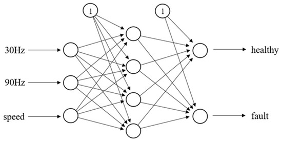
Figure 7.
Structure of Neural Network.
A diagnosis model was constructed by using 200 data of motors No. 1 and No. 2. A datum consisted of three features: values of sideband components around 30 and 90 Hz of load current, and rotating speed. An average accuracy of 99.5% was obtained by 5-fold cross-validation, which was carried out in the same manner as described in Section 4.1.
Evaluation of the constructed model was performed for target motors (No. 3 to No. 6). Table 4 shows the result of the diagnosis. In any case, the accuracy rate is higher than 89% and considered acceptable. Especially, RF achieves the highest accuracy in bearing condition classification.

Table 4.
Diagnosis result based on Neural Network.
5. Discussion
5.1. Comparison with the Previous Method for Diagnosis Accuracy
The authors proposed a fault diagnosis method [14], where the sidebands of the rotating frequency, that is around 30 and 90 Hz component, are treated as features, and the diagnosis was conducted using an SVM. In this diagnosis, the rotation speed is not used as a feature. Here, diagnosis accuracy is obtained by this method and compared with accuracy shown in Section 4, which is obtained by considering the rotating speed.
Diagnosis models of SVM, RF, and NN were constructed in the same manner as described in Section 4.1, Section 4.2, and Section 4.3, respectively. An average accuracy of 74.5%, 66.0%, and 69.0% was obtained by 5-fold cross-validation for each model. Accuracy is lower in any model, indicating that rotation speed may make sufficient contribution to accuracy.
Evaluation of the constructed models was performed for target motors (No. 3 to No. 6). The results using SVM are shown in Table 5. Compared with the results shown in Table 2, the accuracy rate is lower. SVM can overcome the overlapping program using a hyperplane, but it seemed to have a limit. It is confirmed that the rotation speed is an important and effective feature in diagnosis.

Table 5.
Diagnosis result based on SVM.
The other machine-learning algorithms, RF and NN, were also evaluated. The results are shown in Table 6 and Table 7, respectively. Their accuracy is lower by comparing with the result shown in Table 3 and Table 4.

Table 6.
Diagnosis result based on Random Forest.

Table 7.
Diagnosis result based on Neural Network.
When only the sidebands components of the load current spectrum were used as features, it was difficult to solve the overlapping problem of the feature distribution. Because excellent diagnosis results are obtained regardless of the type of machine learning, the combination of the amplitude of the sidebands of load current spectrum, as well as rotating speed, are powerful features for diagnosing a slight bearing fault in various rotating speeds.
5.2. Evaluation of Effect of Fluctuation in Power Supply
So far, data with rotating speeds between 1780 and 1730 min−1 have been discussed. They were obtained by varying the load with the resulting applied voltage ranging between 195 and 205 V. This condition is denoted as Case 1. Because a greater variation in the rotating speed is likely to occur at the site because of greater fluctuation of voltage at distribution panels, an additional experiment and analysis were performed as follows: The voltage applied to the motor was set between 180 and 220 V using a variable transformer under a fixed load, resulting in a rotating speed between 1780 and 1730 min−1. This condition is denoted as Case 2. The voltage range was determined by considering the allowable voltage range of the Japanese 200 V distribution system (182–222 V) and the voltage acceptable for the motor operation (200 V ± 10%).
A new motor (denoted as No. 7) was prepared and the three features were measured under Cases 1 and 2. The three-dimensional feature distribution is shown in Figure 8. The features obtained under Cases 1 and 2 are shown in the red circle and green square, respectively. Features of the two cases are distributed in almost the same region because both features are obtained for the motor with a healthy bearing. It is also confirmed that variation in features is larger in Case 2 because of the larger voltage fluctuation.
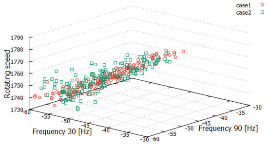
Figure 8.
Effect of voltage fluctuation range of power supply on feature distribution of a healthy motor.
The diagnosis for the No. 7 motor was performed using three machine-learning algorithms. The accuracy of the diagnostic results for the motor is shown in Table 8. Excellent accuracy is obtained regardless of the type of machine learning even when the voltage fluctuation is larger, as in Case 2. This is a favorable characteristic for practical use.

Table 8.
Diagnosis result for No. 7 motor based on machine learning.
5.3. Further Evaluation of Proposed Diagnosis Models
The generalization performance of three proposed diagnosis systems was discussed in Section 4 by 5-fold cross-validation using data obtained for motors No. 1 and No. 2. In this section, the cross-validation is performed using much data obtained for motors No. 1 to No. 6.
Four datasets of healthy motors (No. 1, No. 3 to No. 5) and two datasets of faulty motors (No. 2 and No. 6) are merged in a dataset. Thus, the number of the merged dataset was 748. The merged dataset was divided into five folds randomly. Four folds have 150 data each and the remaining fold has 148 data. The number of data of healthy and faulty motors is different by fold. Four folds are used for training and the remaining fold is used for test. Five-fold cross-validation was carried out.
When a datum has three features (two sideband components of lead current spectrum and rotating frequency), the accuracy rate of an arbitrary case was 96.8%, 96.7%, and 96.9% for SVM, RF, and NN models, respectively. In the case using data consisting of two features (sideband components of lead current spectrum), the accuracy rate for the same case was 84.0%, 85.6%, and 87.3% for SVM, RF, and NN models, respectively.
Compared with accuracy described in Section 5.1, two-feature models by increasing the amount of data. However, accuracy of three-feature models is still higher than that of two-feature models, suggesting that rotation speed plays an important role in diagnosis. In other words, the proposed diagnosis method in this paper is superior to the previous one.
6. Conclusions
This study proposed a reliable fault diagnosis method for the bearing while changing the rotating speed of the motor. First, the bearing fault was replicated and the load current was measured at that time. Second, the problem involved in previous studies was clarified. Then, the load current analysis was performed and three physical quantities (the sidebands, which depend on the rotating frequency and rotating speed) were selected as features. Finally, by using the features, three machine-learning methods (SVM, RF, and NN) were used to diagnose the bearing fault.
The results of this study can be summarized as follows:
1. Rotating speed is an important feature for accurately diagnosing a bearing fault.
2. The amplitude of the sidebands of around 30 and 90 Hz components of load current spectrum and rotating speed are considered selective features because the three-dimensional feature distribution clarifies the difference between healthy and fault bearings.
3. Regardless of the machine-learning algorithm used for bearing fault diagnosis, high diagnostic accuracy is obtained by adding rotating speed as a new feature. Accuracy of approximately 90–100% is achieved, which is improved by approximately 5–60% compared with results obtained without rotating speed.
4. Machine learning-based diagnostic methods can detect a small hole on a bearing of 0.5 mm diameter, potentially paving the way for developing a technique for early fault detection and tracking of its progression.
The application of the diagnosis method to other bearing faults, such as a small scratched or rubbed fault, abrasion will be investigated in a future study. Furthermore, experiments of motors of other specifications, operation frequency will be planned as a next step.
Author Contributions
Conceptualization, H.N. and Y.M.; methodology, H.N.; validation, H.N. and Y.M.; formal analysis, H.N. and Y.M.; investigation, H.N. and Y.M.; resources, H.N. and Y.M; data curation, H.N. and Y.M.; writing—original draft preparation, H.N.; writing—review and editing, H.N. and Y.M.; visualization, H.N.; supervision, H.N. and Y.M.; project administration, H.N.; funding acquisition, H.N. and Y.M. All authors have read and agreed to the published version of the manuscript.
Funding
This research received no external funding.
Institutional Review Board Statement
Not applicable.
Informed Consent Statement
Not applicable.
Data Availability Statement
Not applicable.
Conflicts of Interest
The authors declare no conflict of interest.
References
- IEEE Motor Reliability Working Group. Report of large motor reliability survey of industrial and commercial installations. IEEE Trans. Ind. Appl. 1985, 1A-21, 853–872. [Google Scholar]
- Zhou, W.; Lu, B.; Habetler, T.; Harley, R. Incipient bearing fault detection via motor stator current noise cancellation using wiener filter. IEEE Trans. Ind. Appl. 2009, 45, 1309–1317. [Google Scholar] [CrossRef]
- Jin, X.; Zhao, M.; Chow, T.; Pecht, M. Motor bearing fault diagnosis using trace ratio linear discriminant analysis. IEEE Trans. Ind. Electron. 2014, 61, 2441–2451. [Google Scholar] [CrossRef]
- Tyagi, S.; Panigrahi, S.K. A DWT and SVM based method for rolling element bearing fault diagnosis and its comparison with Artificial Neural Networks. J. Appl. Comput. Mech. 2017, 3, 80–91. [Google Scholar]
- Skora, M.; Ewert, P.; Kowalski, C.T. Selected Rolling Bearing Diagnostic Methods in Wheel Embedded Permanent Magnet Brushless Direct Current Motors. Energies 2019, 12, 4212. [Google Scholar] [CrossRef] [Green Version]
- Kang, M.; Kim, J.; Kim, J.-M. High-performance and energy-efficient fault diagnosis using effective envelope analysis and denoising on a general-purpose graphics processing unit. IEEE Trans. Power Electron. 2015, 30, 2763–2776. [Google Scholar] [CrossRef]
- Caesarendra, W.; Kosasih, P.B.; Tieu, A.K.; Moodie, C.A.S.; Choi, B.-K. Condition monitoring of naturally damaged slow speed slewing bearing based on ensemble empirical mode decomposition. J. Mech. Sci. Technol. 2013, 27, 2253–2262. [Google Scholar] [CrossRef]
- Kang, M.; Kim, J.; Wills, K.M.; Kim, J.M. Time-Varying and Multiresolution Envelope Analysis and Discriminative Feature Analysis for Bearing Fault Diagnosis. IEEE Trans. Ind. Electron. 2015, 62, 7749–7761. [Google Scholar] [CrossRef]
- Mohammed, A.; Djurovic, S. Electric Machine Bearing Health Monitoring and Ball Fault Detection by Simultaneous Thermo-Mechanical Fiber Optic Sensing. IEEE Trans. Energy Convers. 2021, 36, 71–80. [Google Scholar] [CrossRef]
- Nakamura, H.; Asano, K.; Usuda, S.; Mizuno, Y. A Diagnosis Method of Bearing and Stator Fault in Motor Using Rotating Sound Based on Deep Learning. Energies 2021, 14, 1319. [Google Scholar] [CrossRef]
- Blodt, M.; Chabert, M.; Regnier, J.; Faucher, J. Mechanical load fault detection in induction motors by stator current time–frequency analysis. IEEE Trans. Ind. Appl. 2006, 42, 1454–1463. [Google Scholar] [CrossRef]
- Lau, E.C.C.; Ngan, H.W. Detection of motor bearing outer raceway defect by wavelet packet transformed motor current signature analysis. IEEE Trans. Instrum. Meas. 2010, 59, 2683–2690. [Google Scholar] [CrossRef]
- Frosini, L.; Bassi, E. Stator current and motor efficiency as indicators for different types of bearing faults in induction motors. IEEE Trans. Ind. Electron. 2010, 57, 244–251. [Google Scholar] [CrossRef]
- Pandarakone, S.E.; Mizuno, Y.; Nakamura, H. Distinct Fault Analysis of Induction Motor Bearing Using Frequency Spectrum Determination and Support Vector Machine. IEEE Trans. Ind. Appl. 2017, 53, 3049–3056. [Google Scholar] [CrossRef]
- Codoy, W.F.; Morinigo-Sotelo, D.; Deque-Perez, O.; da Silva, I.N.; Goedtel, A.; Palacios, R.H.C. Estimation of Bearing Fault Severity in Line-Connected and Inverter-Fed Three-Phase Induction Motors. Energies 2020, 13, 3481. [Google Scholar]
- Barcelos, A.S.; Cardoso, A.J.M. Current-Based Bearing Fault Diagnosis Using Deep Learning Algorithms. Energies 2021, 14, 2509. [Google Scholar] [CrossRef]
- Zhang, S.; Wang, B.; Kanemaru, M.; Lin, C.; Liu, D.; Miyoshi, M.; Teo, K.H.; Habetler, T.G. Model-Based Analysis and Quantification of Bearing Faults in Induction Machines. IEEE Trans. Ind. Appl. 2020, 56, 2158–2170. [Google Scholar] [CrossRef]
- Devaney, M.J.; Eren, L. Detecting motor bearing faults. IEEE Instrum. Meas. Mag. 2004, 7, 30–50. [Google Scholar] [CrossRef]
- He, M.; He, D. Deep Learning Based Approach for Bearing Fault Diagnosis. IEEE Trans. Ind. Appl. 2017, 53, 3057–3065. [Google Scholar] [CrossRef]
- Boudinar, A.H.; Benouzaa, N.; Bendiabdellah, A.; Khodja, M.E.I.A. Induction Motor Bearing Fault Analysis Using a Root-MUSIC Method. IEEE Trans. Ind. Appl. 2016, 52, 3851–3860. [Google Scholar] [CrossRef]
- Valeria, C.M.N.; Leite, J.G.B.; da Silva, G.F.C.; Veloso, L.E.B.; da Silva, G.; Lambert-Torres, E.L.; Bonaldi, L.E.; de Oliveira, D.L. Detection of Localized Bearing Faults in Induction Machines by Spectral Kurtosis and Envelope Analysis of Stator Current. IEEE Trans. Ind. Electron. 2015, 62, 1855–1865. [Google Scholar]
- Saucedo-Dorantes, J.J.; Delgado-Prieto, M.; Osornio-Rios, R.A.; Romero-Troncoso, R.J. Multifault Diagnosis Method Applied to an Electric Machine Based on High-Dimensional Feature Reduction. IEEE Trans. Ind. Appl. 2017, 53, 3086–3097. [Google Scholar] [CrossRef] [Green Version]
- Hamadache, M.; Lee, D.; Veluvolu, K.C. Rotor Speed-Based Bearing Fault Diagnosis (RSB-BFD) Under Variable Speed and Constant Load. IEEE Trans. Ind. Electron. 2015, 62, 6486–6495. [Google Scholar] [CrossRef]
- Sako, T. Development of the Condition Monitoring Technology for Processing Assembly Plant. In Proceedings of the 13th Symposium on Evaluation and Diagnosis, Kitakyusyu, Fukuoka, Japan, 11–12 December 2014. [Google Scholar]
- Yu, Y.; Dackermann, U.; Li, J.; Subhani, M. Condition Assessment of Timber Utility Poles Based on a Hierarchical Data Fusion Model. J. Comput. Civ. Eng. 2016, 30, 04016010. [Google Scholar] [CrossRef]
- Muzzammel, R.; Raza, A. A Support Vector Machine Learning-Based Protection Technique for MT-HVDC Systems. Energies 2020, 13, 6668. [Google Scholar] [CrossRef]
- Kang, J.; Wang, Z.; Soares, C.G. Condition-Based Maintenance for Offshore Wind Turbines Based on Support Vector Machine. Energies 2020, 13, 3518. [Google Scholar] [CrossRef]
Publisher’s Note: MDPI stays neutral with regard to jurisdictional claims in published maps and institutional affiliations. |
© 2022 by the authors. Licensee MDPI, Basel, Switzerland. This article is an open access article distributed under the terms and conditions of the Creative Commons Attribution (CC BY) license (https://creativecommons.org/licenses/by/4.0/).

