Abstract
Detection of partial discharge (PD) in switchgears requires extensive data collection and time-consuming analyses. Data from real live operational environments pose great challenges in the development of robust and efficient detection algorithms due to overlapping PDs and the strong presence of random white noise. This paper presents a novel approach using clustering for data cleaning and feature extraction of phase-resolved partial discharge (PRPD) plots derived from live operational data. A total of 452 PRPD 2D plots collected from distribution substations over a six-month period were used to test the proposed technique. The output of the clustering technique is evaluated on different types of machine learning classification techniques and the accuracy is compared using balanced accuracy score. The proposed technique extends the measurement abilities of a portable PD measurement tool for diagnostics of switchgear condition, helping utilities to quickly detect potential PD activities with minimal human manual analysis and higher accuracy.
1. Introduction
A power distribution system includes a complex electricity supply network in the form of electrical grids which consist of huge number of power assets such as switchgears, transformers and power cables. Installed decades ago and nearing the end of their useful life, the condition of these equipment needs to be monitored and potentially improved to avoid major disruption. The monitoring and management of such complex network represents a major challenge for utilities and facility owners. According to statistics, nearly 40% of the faults in switchgears originate from insulation faults or potential defects such as cracks in the insulator [1], bad electrical contacts, and dirt contamination or dust ingression of the insulating bush. These insulation defects can excite partial discharge (PD) under electric fields that are hazardous to insulation. PD is also the consequence of local electrical stress concentrations in the insulation or on the surface of the insulation [2]. If PD goes undetected, it will cause safety hazards, power outages and equipment damage [3].
Measurements of ultra-high-frequency (UHF), acoustical emission and transient earth voltage (TEV) signals have been used to monitor PD activity based on the phenomena of electromagnetic radiation, acoustic radiation, and transient current flow that accompany PDs, respectively [4]. However, the detection of PD operationally is an extremely time-consuming process. PD measurements in substations are usually performed manually using professional PD instrumentation with scheduled testing periods and are conducted while the system is in-service [5] to avoid the need to shut down equipment. The diagnosis of the PD measurement data is typically achieved by having a trained engineer study the Phase-Resolved Partial Discharge (PRPD) plots after the data collection process. This also is a very manual and time-consuming process. There are some automated tools available but they require the data to be captured “in-phase”. At the substations, the network is a three-phase system with L1, L2 and L3 phases. The PD can happen at any of the phases, while the engineer at site can only use the PD tools to acquire the voltage phase reference through power socket or substation light sources. Thus, the PRPD measured is with a phase shift, i.e., not “in-phase”. It is challenging for the engineer to obtain “in-phase” PRPD measurement at the substation, which can otherwise easily be performed in a lab environment. As such, most of the existing literature discusses the simulation of partial discharge data in a lab environment, hence assuring that the captured data will be “in-phase”.
There have been multiple reviews on the techniques used to automatically detect the presence of PD [6,7,8,9]. Most research work [10,11,12] focuses on using experimentally simulated PD data obtained in the lab. These research works typically focus more on model training, testing, and tuning processes. Such simulated experimental lab data pose at least three concerns:
- Noisy: Data obtained from live environments are often noisy. Although some of the literature has attempted to re-create noise, such augmentations are typically limited. Often, they are unable to replicate the full spectrum of noise present in the actual environment.
- Phase shifted: Data obtained from live environments are often phase-shifted. Most techniques presented in the literature assume that the captured PD data is in-phase. However, this is not the case because it is highly likely that the PD data captured on site at the substations will not be in phase.
- Stochastic: Data from live environments would be very varied as they are obtained from different substations. There is also the possibility of detecting different type of PD activities, which may not be well represented in lab experiments.
Research work in recent years has started to focus on using the techniques on real, live operational data, as in [13,14]. For these papers, the focus has shifted entirely to that of data cleaning and feature extraction. It may be inferred that applying model training wholesale without good cleaning and extraction may not yield good results. The proposed technique presented in this paper employs a clustering method for feature extraction such that partial discharges with PRPD plots captured out-of-phase can still be detected. This technique is expected to extend the capabilities of portable PD measurement tools to provide more accurate and faster diagnostics of PD activities in switchgears.
2. Literature Review
The literature review is divided into three sub-sections to address the different sub-problems encountered when performing PD diagnostics, namely, noise removal, feature extraction and machine learning algorithms.
2.1. Noise Removal
Two of the main challenges in noise removal are: (1) the removal of the noise despite high levels of variability in the data and (2) the removal of noise data while retaining the actual PRPD points. PRPD data are a 2D plot of the partial discharge activity relative to the 360 degrees of an Alternating Current (AC) cycle. Hence, the x-coordinates represent 360 degrees and there are only 360 points on the x-axis. The y-axis represents the amplitude (in dBmV for transient earth voltage measurements) of each discharge event. The PRPD plot is measured based on 10 s of recording.
This paper will review three different forms of noise removal techniques for the PRPD data. These techniques will be applied to the PRPD plots (Figure 1) and will demonstrate some of the issues faced by these techniques. The three techniques reviewed are: (1) erosion (a type of image processing technique), (2) Discrete Wavelet Transformations (DWT) and (3) Fast Fourier Transformation (FFT).
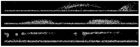
Figure 1.
Examples of positive PRPD samples. Top: Internal discharge, Middle: Internal discharge from 22 kV bushing of oil-filed transformer, Bottom: Internal discharge from voids of solid insulator.
2.1.1. Erosion
Some of the basic forms of noise removal include techniques such as morphological filters, such as erosion. This form of noise removal has been shown to be effective for salt and pepper noise. Hence, it can remove random points within the PRPD plot that can be classified as noise. Running such an erosion algorithm on the plot may yield a plot where way too much data have been removed and the white noise remains. This is due to the small sizes of the images and the relatively low repetition rate of the points. Hence, such erosion techniques tend to also remove the essential data from the image, as seen in Figure 2. In this situation, the data from Figure 1 were passed through a 2 × 2 erosion filter and the figure shows that the number of datapoints has been very much removed.
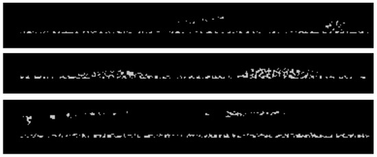
Figure 2.
Data from Figure 1 after going through an 2 × 2 erosion filter.
2.1.2. Discrete Wavelet Transformations
Wavelet transforms have been claimed to be an effective way to remove noise in PRPD plots [3,15]. Two of the highlighted wavelet transformations were DB.5 and bior1.5. Testing both techniques on the operational data from Section II yields the results shown in Figure 3. Visually, this indicates that certain forms of white noise persist even after these wavelet transformations.
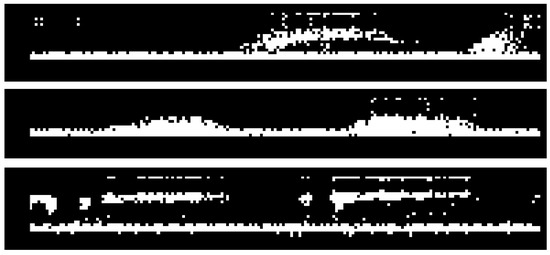
Figure 3.
Data from Figure 1 after undergoing a db5 wavelet transform.
2.1.3. Fast Fourier Transform
The final form of noise removal technique is via Fast Fourier Transform. This technique breaks down the plot into frequency domain, carries out a removal of lower value frequencies and reconstructs the frequencies back to the image. The removal of white noise is essential because it may affect the quality of the generated features and, subsequently, the quality of the machine learning model. As shown in Figure 4, these existing techniques may not be adequate in the removal of white noise in the PRPD plot. The paper will propose a white noise removal technique in Section 4.1.
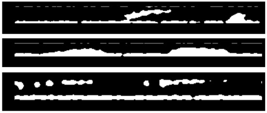
Figure 4.
Data from Figure 1 after going through a deconstruction and reconstruction via FFT.
2.2. Feature Extraction
2.2.1. Feature Extraction in Lab Generated PD Data
There are three main techniques for feature extraction for PRPD plots [9]. The first technique is based on statistical methods such as mean, skewness or Weibull analysis [16,17]. The second technique is based on the extraction of analytical features such as phase angle patterns from PRPD plots [8,18]. However, these features can be quite susceptible to errors if the plot is phase-shifted. The final technique is based on dimensionality reduction methods such as PCA/t-SNE [16,19]. These dimensionality reduction methods are applied at times on top of the earlier two techniques to reduce the number of inputs into the machine learning algorithm.
2.2.2. Two Methods of Applying Feature Extraction
There are two methods to apply these feature extraction techniques. The first method [17] applies these feature extraction techniques globally across the entire PRPD plot (of 360 degrees). The extraction of features in this manner will be too general, as much of the data will be summarized into a handful of features. Hence, the extracted features may not be the best representation of the data. The second method [12,20,21] tries to solve this by segregating the PRPD plot into segments, with each segment constituting datapoints from a few angles. For instance, if each segment consists of 6 degrees, there will be 60 segments in total. If each segment has 10 degrees, there will be 36 segments in total. The feature extraction technique will then be applied to each of these segments. For instance, if the mean, skewness, and kurtosis are features to be extracted from each segment, and there are 60 segments in total, the total number of features will be 180 (3 × 60) features.
2.2.3. Application of Feature Extraction to Operational Data
A survey of recent prior art on PD detection on operational data [10,13,14] shows that these researchers used specialized techniques for feature extraction. For instance [10] uses a technique known as Histogram of Orientated Gradient (HOG), an image-processing technique used to capture edges in images [22]. Ref. [13] uses a bespoke grid filtering technique. Ref. [14] selects and projects the regions of the PRPD plots. This seems to suggest that these techniques might not work as well on live operational data for the following reasons:
- Phase shifted: Data extracted from live operational conditions will always be shifted in phase. Hence, it will be challenging to apply feature extraction techniques as they require the data to be in-phase.
- Predetermined segmentation of windows: The PRPD plot is subdivided into predetermined plots via grid sizes or phase angles. This may cause issues as the extracted features would not be directly from the regions indicating the presence of PD, but are based on predetermined grid spaces instead. These techniques may work very well if the PRPD plot is in phase, but if the plot is phase-shifted, features may be extracted from grid spaces in partial regions.
- Multiple types of PD in a PRPD plot: In live operational conditions, it would not be surprising to find the presence of multiple different types of PD spread out across different geo-locations. Some of the PRPD plots may also exhibit plots from multiple PD sources.
Hence, in this paper, a new approach is presented, where the features are obtained from the clusters in the PRPD plot. These features will be used to determine the presence of PD across the entire plot, rather than predetermined grid areas. This will be elaborated further in Section 4.3.
2.3. Machine Learning
Based on papers reviewing machine learning classification techniques on PD detection, Refs. [6,7,9] two of the most-used techniques are support vector machines (SVM) [21,23] and artificial neural networks (ANN) [14,20]. Readers are also invited to refer to [8] for a more in-depth discussion on PD detection using ANNs. Recently, deep learning techniques such as Convolutional Neural Networks [11] and Long Short Term Memory (LSTM) [24] have also been used for the classification of PDs. Most of these papers use experimental lab data, and these data may not be generalizable to live operational conditions. In Section 4.4, this paper will showcase the results on the accuracy of PD detection when the extracted features are run across a series of classical machine learning techniques.
3. Operational Data
PD data from distribution substations of local utility company were collected over a six-month period by technicians using handheld devices. These measurement devices provide first-cut information on potential PD activities based on their severity level.
Subsequently, the PRPD plots were manually inspected and labeled into positive and negative plots. This labelling was performed by industrial experts/practitioners from our collaborator, who owns and operates the national power grid. Similarly, different types of partial discharge events were labeled and verified by the industrial experts/practitioners.
In total, 452 pieces of Phase-Resolved Partial Discharge (PRPD) 2D plots were obtained. Out of these, there were 342 negative PRPD plots with no PDs and 110 positive PRPD plots with PDs. These operational data will typically have different forms of PD [25], an overlapping PD and the strong presence of random white noise. For instance, even for internal discharges, the PRPD plots will look vastly different [16]. Examples of these plots can be seen in Figure 1.
As these data are taken from an operational environment, they clearly show the presence of noise known as white noise (WN). This white noise is can be observed as a continuous signal at the bottom of the PRPD plot. A typical machine learning pipeline for classical classification algorithms (such as decision trees, SVM) involves the following iterative steps [13]:
- Data cleaning;
- Feature extraction;
- Model training;
- Model testing;
- Model tuning.
This paper presents a novel way of executing the first two steps: data cleaning and feature extraction of PRPD plots of operational data with WN. Subsequently, various machine learning models will be trained using these features. The performances of these models will be individually compared.
4. Methodology
One of the major concerns in the feature extraction techniques used in prior art is that extraction of features is typically performed globally from the entire PRPD plot (Section 2.2). This causes the extracted features to be sensitive as there are many factors (such as noise and possible phase shifts), which may affect the consistency/generalizability of the extracted features. Hence, one of the main contributions proposed in this paper is the method used to only carry out feature extraction from specific regions of the PRPD plots that indicate the presence of PDs. To achieve this, a series of noise-cleaning mechanisms and unsupervised learning was used to first extract possible PD clusters. The features were then extracted from these individual PD clusters instead of the entire PRPD plot. This will be explained in the subsequent subsections.
4.1. White Noise Removal
Two types of noise are typically seen in condition monitoring [7]. They are white noise (WN) and discrete spectral interference (DSI). The main type of noise in this dataset, however, is white noise. This type of noise typically appears at the lower y-axis values of the PRPD plot. A simple threshold would simply not work as the white noise occurs differs over different datapoints. The use of a histogram would also not be effective as the repetition rate of white noise also varies randomly.
The method proposed is to determine the baseline where the noise occurs for each individual plot and subsequently remove it. To determine this baseline, the intuition is the following: if a PD is present, it presents in the PRPD plot as datapoints hovering over the white noise. To capitalize on this, the intuition is to determine if there are two clusters of points available, and if there are, to determine the baseline of the white noise of the lower cluster. The algorithm for determining the baseline of the lower WN cluster is the following:
- Bucketing: The PRPD plot consists of 360 degree phases in the x-axis. These 360-degree are divided into 36 buckets for i ranging from 0 to 35. Each bucket will have datapoints from 10 phase angles. For instance, phase angles from 0 to 9 will fall under the first bucket, phase angles from 10 to 19 to the second, etc.
- Clustering: For each of these buckets , a simple k-means that the clustering algorithm is carried out with the number of clusters set to two. Clustering is then carried out based only on the y-values (voltage value) alone. The k-means algorithm is randomly seeded. However, as it is run through the 36 buckets of the PRPD plot, the results are stable. There are only two possible outcomes of this clustering. In the first outcome, a PD may be present and the clusters are spaced far apart. In the second outcome, a PD is not present and the two clusters are spaced close to one another, within the region of the WN. The rationale for stating that just two outcomes (spaced far and spaced close) are possible is based on the assumption that the PRPD plot consists of two types of data, the whitenoise versus the partial discharge voltage values. The assumption is also that the white noise tends to occupy the lower voltage values but is typically constant throughout the entire PRPD plot.
- Bucket Baseline Determination: For each bucket , a baseline is calculated in the following manner. In the first outcome, where the clusters are far apart in that bucket, the highest point of the lower cluster is chosen as . If the two clusters are spaced close to one another, the centroid of the higher cluster is chosen as . The rationale for choosing the baseline is to determine the whitenoise voltage level present in the PRPD plot. In the first outcome, where the two centroids are spaced far apart, the lower centroid is chosen as the baseline. In the second outcome, where the two centroids are spaced close to one another, the higher centroid is chosen as the baseline. Kmeans is run on each bucket to find the two centroids. If the distance between the centroids falls below a certain threshold, it is deemed to fall under the second outcome. However, if the distance between the centroids is large, it is deemed to fall under the first outcome.
- Plot Baseline Determination: The mode of the 36 bucket baselines is finally calculated and chosen as the baseline value for the PRPD plot. Subsequently, all points in the PRPD plot where it falls below will be removed. This generates the plot seen in Figure 5.
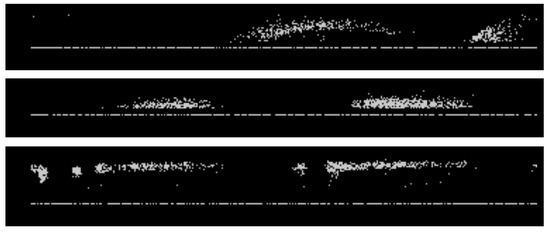 Figure 5. Data from Figure 4 after removal of datapoints below .
After the white noise is removed, the next step is to determine the exact location of the PD clusters. This will be described in the subsequent subsection.
4.2. Clustering of PD Clusters
Typical clustering techniques (such as k-means) requires datapoints to be organized around a centroid, a scenario which typically would not occur in our case. A better class of clustering algorithms would be that of density-based clustering (DBScan [26] or HDBScan [27]), where the clusters are arranged according to the inter-point distances.
The intuition behind HDBScan is the following: For all point pairs, calculate a metric that determines how reachable these two points are from each other. This metric, known as the mutually reachable distance [27] will generate a low score if they are in the vicinity of each other, but will have a higher score otherwise.
This step creates a score to all edges between the points. A minimum spanning tree [28] is constructed to determine the lowest collective scores between all these points. A cluster hierarchy is then built based on the minimum spanning tree. An example of the final outcome of both the clusters and dendogram can be seen in Figure 6. It can be seen in the hierarchy that datapoints split off from a cluster where the width of the line represents the number of points in the cluster. Interested readers are invited to refer to [27,29] for a more in-depth explanation.
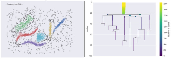
Figure 6.
An example of how HDBScan works. Left image shows how clusters are formed based on the inter-points’ distance. Right image shows how clusters are arranged in a hierarchical manner as a dendrogram. Image reference from [29].
HDBScan was chosen because it is less sensitive to initial parameters (as compared to DBScan) and, since the clusters are arranged in a hierarchical manner, the number of clusters extracted based on the data can be controlled. In this paper, the proposed approach uses the hierarchy within the dendogram to extract only four clusters or fewer per PRPD plot.
The rationale for four or fewer clusters is because PRPD plots rarely, if ever, have more than four clusters in the plot. This can be validated through the typical PRPD patterns library. Using more clusters would create clusters that are too small, which may not capture the shape of the partial discharge cluster.
Examples of an extraction of these clusters can be seen in Figure 7. The extracted clusters are indicative of potential discharge in the PRPD plot. It can be said that the feature-extraction technique can extract the features of positive PRPD plots, which are vastly different. Features from these clusters will be extracted in the next section and used as independent variables for the various machine learning algorithms in Section 4.4.
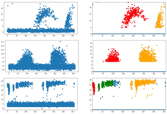
Figure 7.
An example of how HDBScan is applied to the sample images of the dataset. Left column shows the original dataset. Right column shows the clustered data after white noise removal. The colors red, yellow and green show the different clusters achieved from HDBScan.
4.3. Feature Extraction
Finally, the cluster features can be extracted from these individual clusters. In most prior work, features were extracted from the entire PRPD plot. However, the presence of PRPD is typically determined through the presence of a few unique shapes of the plot in specific areas. Hence, the paper proposes the extraction of features based only from the clusters.
Four features were extracted from each cluster. These are the length of the cluster, height of the cluster, gradient from top right to bottom left of the cluster and gradient from top left to bottom right of the cluster. The definitions of these four features are provided below.
- Length of the cluster: Within a cluster, the rightmost x-value deducted from the leftmost x-value.
- Height of the cluster: Within a cluster, the top y-value deducted from the bottom y-value.
- Gradient from top right to bottom left of the cluster: Within a cluster, this gradient is calculated from the point with the largest y-value and rightmost x-value to the point with the lowest y-value and leftmost x-value.
- Gradient from top left to bottom right of the cluster: Within a cluster, this gradient is calculated from the point with the largest y-value and leftmost x-value to the point with the lowest y-value and rightmost x-value.
The rationale for using these four features of the PRPD plots is because they are able to distinguish between true PD clusters versus noise or interference. A simple ablation study was performed to illustrate this and the results are presented in Table 1. These four features are finally fed into various machine learning algorithms and their accuracy rates are compared.

Table 1.
Balanced Accuracy Result Comparison.
4.4. Classification Results
Three main types of classification techniques were used on the extracted features:
- Linear Methods: Logistic Regression and Neural Networks;
- Tree-Based Methods: Decision trees as well as ensemble methods such as Random Forest (Bagging) and XGBoost (Boosting);
- Kernel Methods: Support Vector Machines.
A metric known as the balanced accuracy score [30] was used to compare the results of all these individual techniques. The balanced accuracy score is chosen because it is a better comparison indicator when the dataset is imbalanced. As there are only two classes in our dataset, the balanced accuracy score is defined as:
In addition to the balanced accuracy score, two other metrics, false positives and false negatives, were also considered. In our context, false positives are the prediction that the sample has a PD when it does not. False negatives are the prediction that the sample does not have a PD when it does. The cost associated with a false positive will be a reduction of productivity (where staff is deployed to perform a manual confirmation check to verify the presence of a PD) while the cost associated with a false negative may potentially be extremely damaging, including blackouts.
The results of these algorithms are shown in Table 2. Decision Tree and XGBoost algorithms perform best, with a balanced accuracy of 0.95. Typically, ensemble techniques such as Random Forests or XGBoost perform better than their single-model counterparts such as Decision Trees. However, due to the small size of the test dataset (about 122), it is observed that the three forms of tree-based methods do not show a large difference in balanced accuracy and, in fact, Decision Trees slightly outperform XGBoost by not having any false negatives. It is, however, interesting to note that, in the current dataset, these tree-based techniques seem to work slightly better than both neural networks and SVM.
Table 2.
Balanced Accuracy Result Comparison.
Typically, the business objective requires the number of false negatives to be kept at a minimum; therefore, based on the limited set of data in the experiment, tree-based methods such as decision trees, random forests or XGBoost would be most suitable.
A simple ablation study for the features is given in the table below. Assume the features are named F1, F2, F3 and F4 for length, height, gradient from top right to bottom left, and gradient from top left to bottom right, respectively. The numbers show the balanced accuracy scores based on the models in the first column. From this simple ablation study, we can deduce that the accuracy scores exhibit the highest accuracy and stability when we utilize all four features.
5. Conclusions
In this paper, a clustering technique was presented for data cleaning and feature extraction of phase-resolved partial discharge (PRPD) plots obtained from real, live substation environments. The 425 live data that were obtained show the strong presence of random white noise and positive PD plots have overlapping PDs. The proposed clustering technique performs a series of noise-cleaning mechanisms and unsupervised learning to first extract possible PD clusters. Subsequently, features were extracted from the individual PD clusters instead of the entire PRPD plot. Using the proposed methodology, four features were extracted from each PD cluster, namely, the length of the cluster, height of the cluster, gradient from top right to bottom left of the cluster and gradient from top left to bottom right of the cluster. Based on the obtained results, the proposed data-cleaning process was successful in removing significant white noise in the live data. The feature extraction technique was able to extract the features of positive PRPD plots, which are vastly different. The extracted features were fed into six different machine-learning algorithms and the accuracy was evaluated. Using a small size of test dataset (about 122 plots), it was found that the tree-based techniques seem to work slightly better than both neural networks and SVM techniques. In particular, Decision Tree and Random Forest algorithms performs best with zero false negatives. This is probably due to the relatively small data size, and a larger data size would better generalize the results. The developed technique is expected to extend the measurement capabilities of a portable PD measurement tool for more accurate diagnostics of switchgear condition monitoring by helping utilities to quickly detect potential PD activities and avoiding costly shutdowns.
Author Contributions
Conceptualization, D.S., J.A., L.K.X. and S.B.K.; methodology, D.S., J.A., L.K.X. and S.B.K.; software, D.S. and J.A.; validation, D.S., J.A. and L.K.X.; formal analysis, D.S., J.A. and L.K.X.; investigation, D.S., J.A. and L.K.X.; resources, T.K.J. and J.F.Y.; data curation, D.S., J.A. and L.K.X.; writing—original draft preparation, D.S. and S.B.K.; writing—review and editing, D.S. and S.B.K.; visualization, D.S. and S.B.K.; supervision, T.K.J. and J.F.Y.; project administration, T.K.J. and J.F.Y.; funding acquisition, T.K.J. and J.F.Y. All authors have read and agreed to the published version of the manuscript.
Funding
This work was supported in part by Singapore Institute of Technology (SIT) and the SP Group.
Institutional Review Board Statement
Not applicable.
Informed Consent Statement
Not applicable.
Conflicts of Interest
The authors declare no conflict of interest. The funders had no role in the design of the study; in the collection, analyses, or interpretation of data; in the writing of the manuscript, or in the decision to publish the results.
References
- Sarathi, R.; Umamaheswari, R. Understanding the partial discharge activity generated due to particle movement in a composite insulation under AC voltages. Int. J. Electr. Power Energy Syst. 2013, 48, 1–9. [Google Scholar] [CrossRef]
- Kessler, O. The Importance of Partial Discharge Testing: PD Testing Has Proven to Be a Very Reliable Method for Detecting Defects in the Insulation System of Electrical Equipment and for Assessing the Risk of Failure. IEEE Power Energy Mag. 2020, 18, 62–65. [Google Scholar] [CrossRef]
- Montanari, G.C.; Cavallini, A. Partial discharge diagnostics: From apparatus monitoring to smart grid assessment. IEEE Electr. Insul. Mag. 2013, 29, 8–17. [Google Scholar] [CrossRef]
- Zhe, W. Analysis of TEV Caused by Partial Discharge of Typical Faults in HV Switchgear. High Volt. Appar. 2014, 2, 60–67. [Google Scholar]
- Stone, G.C. A perspective on online partial discharge monitoring for assessment of the condition of rotating machine stator winding insulation. IEEE Electr. Insul. Mag. 2012, 28, 8–13. [Google Scholar] [CrossRef]
- Lu, S.; Chai, H.; Sahoo, A.; Phung, B.T. Condition Monitoring Based on Partial Discharge Diagnostics Using Machine Learning Methods: A Comprehensive State-of-the-Art Review. IEEE Trans. Dielectr. Electr. Insul. 2020, 27, 1861–1888. [Google Scholar] [CrossRef]
- Luo, Y.; Li, Z.; Wang, H. A Review of Online Partial Discharge Measurement of Large Generators. Energies 2017, 10, 1694. [Google Scholar] [CrossRef]
- Mas’ud, A.A.; Albarracín, R.; Ardila-Rey, J.A.; Muhammad-Sukki, F.; Illias, H.A.; Bani, N.A.; Munir, A.B. Artificial Neural Network Application for Partial Discharge Recognition: Survey and Future Directions. Energies 2016, 9, 574. [Google Scholar] [CrossRef]
- Wu, M.; Cao, H.; Cao, J.; Nguyen, H.L.; Gomes, J.B.; Krishnaswamy, S.P. An overview of state-of-the-art partial discharge analysis techniques for condition monitoring. IEEE Electr. Insul. Mag. 2015, 31, 22–35. [Google Scholar] [CrossRef]
- Song, S.; Qian, Y.; Wang, H.; Zang, Y.; Sheng, G.; Jiang, X. Partial Discharge Pattern Recognition Based on 3D Graphs of Phase Resolved Pulse Sequence. Energies 2020, 13, 4103. [Google Scholar] [CrossRef]
- Florkowski, M. Classification of Partial Discharge Images Using Deep Convolutional Neural Networks. Energies 2020, 13, 5496. [Google Scholar] [CrossRef]
- Mas’ud, A.A.; Ardila-Rey, J.A.; Albarracín, R.; Muhammad-Sukki, F. An Ensemble-Boosting Algorithm for Classifying Partial Discharge Defects in Electrical Assets. Machines 2017, 5, 18. [Google Scholar] [CrossRef]
- Araújo, R.C.F.; de Oliveira, R.M.S.; Brasil, F.S.; Barros, F.J.B. Novel Features and PRPD Image Denoising Method for Improved Single-Source Partial Discharges Classification in On-Line Hydro-Generators. Energies 2021, 14, 3267. [Google Scholar] [CrossRef]
- de Oliveira, R.M.S.; Araújo, R.C.F.; Barros, F.J.B.; Segundo, A.P.; Zampolo, R.F.; Fonseca, W.; Dmitriev, V.; Brasil, F.S. A System Based on Artificial Neural Networks for Automatic Classification of Hydro-generator Stator Windings Partial Discharges. J. Microwaves Optoelectron. Electromagn. Appl. 2017, 16, 628–645. [Google Scholar] [CrossRef]
- Mostarac, P.; Malarić, R.; Mostarac, K.; Jurčević, M. Noise Reduction of Power Quality Measurements with Time-Frequency Depth Analysis. Energies 2019, 12, 1052. [Google Scholar] [CrossRef]
- Lai, K.X.; Phung, B.T.; Blackburn, T.R. Application of data mining on partial discharge Part I: Predictive modelling classification. IEEE Trans. Dielectr. Electr. Insul. 2010, 17, 846–854. [Google Scholar] [CrossRef]
- Schober, B.; Schichler, U. Application of Machine Learning for Partial Discharge Classification under DC Voltage. In Proceedings of the Nordic Insulation Symposium, Vapriikki, Finland, 12–14 June 2019; pp. 16–21. [Google Scholar] [CrossRef]
- Chen, P.H.; Chen, H.C.; Liu, A.; Chen, L.M. Pattern recognition for partial discharge diagnosis of power transformer. In Proceedings of the 2010 International Conference on Machine Learning and Cybernetics, Qingdao, China, 11–14 July 2010; Volume 6, pp. 2996–3001. [Google Scholar] [CrossRef]
- Raymond, W.J.K.; Illias, H.A.; Abu Bakar, A.H. High noise tolerance feature extraction for partial discharge classification in XLPE cable joints. IEEE Trans. Dielectr. Electr. Insul. 2017, 24, 66–74. [Google Scholar] [CrossRef]
- Sukma, T.R.; Khayam, U.; Suwarno; Sugawara, R.; Yoshikawa, H.; Kozako, M.; Hikita, M.; Eda, O.; Otsuka, M.; Kaneko, H.; et al. Classification of Partial Discharge Sources using Waveform Parameters and Phase-Resolved Partial Discharge Pattern as Input for the Artificial Neural Network. In Proceedings of the 2018 Condition Monitoring and Diagnosis (CMD), Perth, Australia, 23–26 September; 2018; pp. 1–6. [Google Scholar] [CrossRef]
- Hao, L.; Lewin, P.L. Partial discharge source discrimination using a support vector machine. IEEE Trans. Dielectr. Electr. Insul. 2010, 17, 189–197. [Google Scholar] [CrossRef]
- Dalal, N.; Triggs, B. Histograms of oriented gradients for human detection. In Proceedings of the 2005 IEEE Computer Society Conference on Computer Vision and Pattern Recognition (CVPR’05), San Diego, CA, USA, 20–25 June 2005; Volume 1, pp. 886–893. [Google Scholar] [CrossRef]
- Hao, L.; Lewin, P.; Dodd, S. Comparison of support vector machine based partial discharge identification parameters. In Proceedings of the 2006 IEEE International Symposium on Electrical Insulation, Toronto, ON, Canada, 11–14 June 2006; pp. 110–113. [Google Scholar] [CrossRef]
- Nguyen, M.T.; Nguyen, V.H.; Yun, S.J.; Kim, Y.H. Recurrent Neural Network for Partial Discharge Diagnosis in Gas-Insulated Switchgear. Energies 2018, 11, 1202. [Google Scholar] [CrossRef]
- Reid, A.J.; Judd, M.D.; Fouracre, R.A.; Stewart, B.G.; Hepburn, D.M. Simultaneous measurement of partial discharges using IEC60270 and radio-frequency techniques. IEEE Trans. Dielectr. Electr. Insul. 2011, 18, 444–455. [Google Scholar] [CrossRef]
- Ram, A.; Jalal, S.; Jalal, A.S.; Kumar, M. A Density Based Algorithm for Discovering Density Varied Clusters in Large Spatial Databases. Int. J. Comput. Appl. 2010, 3, 1–4. [Google Scholar] [CrossRef]
- Campello, R.J.G.B.; Moulavi, D.; Sander, J. Density-Based Clustering Based on Hierarchical Density Estimates. In Proceedings of the Advances in Knowledge Discovery and Data Mining, Gold Coast, Australia, 14–17 April 2013; pp. 160–172. [Google Scholar] [CrossRef]
- Pettie, S. Minimum Spanning Trees. Encycl. Algorithms 2008, 541–544. [Google Scholar] [CrossRef]
- McInnes, L.; Healy, J.; Astels, S. hdbscan: Hierarchical density based clustering. J. Open Source Softw. 2017, 2, 205. [Google Scholar] [CrossRef]
- Brodersen, K.H.; Ong, C.S.; Stephan, K.E.; Buhmann, J.M. The Balanced Accuracy and Its Posterior Distribution. In Proceedings of the 20th International Conference on Pattern Recognition, Istanbul, Turkey, 23–26 August 2010; pp. 3121–3124. [Google Scholar] [CrossRef]


Publisher’s Note: MDPI stays neutral with regard to jurisdictional claims in published maps and institutional affiliations. |
© 2022 by the authors. Licensee MDPI, Basel, Switzerland. This article is an open access article distributed under the terms and conditions of the Creative Commons Attribution (CC BY) license (https://creativecommons.org/licenses/by/4.0/).