Multiobjective Optimal Control of Wind Turbines: A Survey on Methods and Recommendations for the Implementation

Abstract

Advanced control system design for large wind turbines is becoming increasingly complex, and high-level optimization techniques are receiving particular attention as an instrument to fulfil this significant degree of design requirements. Multiobjective optimal (MOO) control, in particular, is today a popular methodology for achieving a control system that conciliates multiple design objectives that may typically be incompatible. Multiobjective optimization was a matter of theoretical study for a long time, particularly in the areas of game theory and operations research. Nevertheless, the discipline experienced remarkable progress and multiple advances over the last two decades. Thus, many high-complexity optimization algorithms are currently accessible to address current control problems in systems engineering. On the other hand, utilizing such methods is not straightforward and requires a long period of trying and searching for, among other aspects, start parameters, adequate objective functions, and the best optimization algorithm for the problem. Hence, the primary intention of this work is to investigate old and new MOO methods from the application perspective for the purpose of control system design, offering practical experience, some open topics, and design hints. A very challenging problem in the system engineering application of power systems is to dominate the dynamic behavior of very large wind turbines. For this reason, it is used as a numeric case study to complete the presentation of the paper.

1. Introduction

Control engineering is obligated to evolve in line with world progress, where the mastery of engineering systems is becoming more and more difficult. One characteristic problem is that advanced systems need to fulfill optimality in several ways, where the stated objectives could simultaneously be opposing, conflicting, or complementary. Hence, Multiobjective Optimal Control (MOOC, see e.g., [1,2,3,4] and their references) arose primarily in the last two decades as a helpful instrument to handle these types of control cases. Ongoing survey works about the subject are, for instance, [5,6].

A significant expectation at that point was the thought of finding a general-purpose optimizer able to manage several objectives, with the capacity to address a wide range of control configurations and control operation problems. Nowadays, it is realized that such ideal MOO tools are very difficult to create and that MOO techniques can only undertake a minor number of problems and, in addition, under concrete situations. Furthermore, some algorithms that work correctly in the case of a concrete set of optimization problems are not able to provide acceptable solutions in other cases, where other algorithms perform better [7]. Moreover, experience shows that earlier information about the control problem, the tuning parameters, the numerical behavior of the optimization approach, as well as the objective functions supplemented by much working time is essential before a MOO optimizer yields satisfactory outcomes. This point can be especially frustrating if the sought-after Pareto front is unknown a priori.

While the research in the field of MOO is focused on the obtention of new algorithms, whose aim is to find more complex Pareto frontiers or more accurate solutions by utilizing specially constructed test objective functions, MOO users, for example, control engineers, work with realistic cost functions. In such circumstances, the forms of Pareto fronts are unknown in advance, and consequently, adjusting and tuning of optimization methods is not straightforward. Despite MOO being an extremely effective instrument for solving very complex problems in control system design, its application is not simple.

Furthermore, current design issues appear to be fast gaining in complexity, where the inclusion of several systems with subsystem levels and additional objective functions must also be considered in the optimization procedure. Thus, Pareto methods cannot provide satisfactory results, and bilevel multiobjective optimization can facilitate the possibility of obtaining the desired outcome (see, for instance, [8]). An application of bilevel MOO to a control problem is given in [9].

Hence, the aim of this work, following the previous study [10], is to depict MOO control from a practitioner’s perspective. The remainder of the work will be presented in the following form: The next section, Section 2, is devoted to introducing the concept of multiobjective optimization for the sake of completeness and describing the most important algorithms. Typical objective functions for control are the subject of Section 3, as well as the evaluation procedures analyzed in Section 4. In Section 5, aspects related to decision-making are shown, followed by the application example and the corresponding results in Section 6 and Section 7, respectively. Finally, conclusions are portrayed in Section 8.

2. Some Fundamentals on Multiobjective Optimization

Multiobjective optimization can be found in the literature under several different names, such as, for instance, multiperformance, multicriteria, or vector optimization. It can be described as the activity of obtaining a vector of parameters or decision variables as the outcome of an optimization process carried out on a vector field of objective functions with constraints that have to be satisfied during the operation. These objective functions normally correspond to mathematical descriptions of design specifications that are often in conflict with each other.

2.1. Definitions

The multiobjective optimization problem can be formally stated as

to find	α = [α1 … α np]T or u = [u1 … ul]T,
optimizing	J(u,α) = [J1(u,α) … Jnf(u,α)]T
with respect to	α or to u
subject to	gi(u,α) ≤ 0 and hj(u,α) = 0,
for	i = 1, …, ng, j = 1, …, nh,

where J∈ϑ ⊂ $ℝ$^nf is a vector of objective functions, u∈U ⊂ $ℝ$^l is a vector of decision variables, α∈A ⊂ $ℝ$^np is a vector of parameters, n_f is the number of objective functions, n_g is the number of inequalities constraints and n_h is the number of equality constraints. By optimization, it means either minimization or maximization, depending on the problem to be addressed.

Contrarily to single-objective optimization (SOO), where only a unique global optimal solution exists, there are many optimal equivalent solutions for a MOO problem. Therefore, a definition of the optimum has to be defined in advance. In the present work, the multiobjective Pareto optimality formulated in [11] is assumed.

Definition 1:

A point, α°∈A ⊂ $ℝ$^l, is said to be Pareto optimal with respect to A iff no other point, α∈A, satisfies the conditions J(u,α) ≤ J(u,α°) and J_i(u,α) < J_i(u,α°) for at least one i. This means that it is impossible to enhance a Pareto optimal point without worsening the value of at least one of the other objective functions.

In some cases, it is helpful to reckon with a definition for a suboptimal point that can be reached more easily by the algorithm, and, at the same time, it is an acceptable solution from the practical point of view. This is provided, e.g., by the definition of weakly Pareto optimality.

Definition 2:

A point, α°∈ A ⊂ $ℝ$^l, is said to be weakly Pareto optimal if no other point α∈A, satisfies J(u,α) < J(u,α°).

In other words, a point is weakly Pareto optimal if no other point can improve all objective functions at the same time. Thus, Pareto optimal points are always weakly Pareto optimal, but not the contrary case. All Pareto optimal points constitute the Pareto optimal set defined as

$$\wp \triangleq \left\{\alpha °\in A\subseteq {ℝ}^l|\neg \exists \alpha \in A,\forall i{J}_i(u,\alpha )\le J_i(u,\alpha °)\wedge \exists i:J_i(u,\alpha )<J_i(u,\alpha °)\right\}.$$

(1)

The image ℘_f of the Pareto optimal set ℘ ⊂ U is called Pareto front and is defined in the objective space ϑ.

Definition 3:

Given a vector objective function J(u,α) and the corresponding Pareto optimal set ℘, the Pareto front is defined by

$${\wp }_f\triangleq \left\{J(u,{\alpha }_i)\in \mathbf{\vartheta }\subseteq {ℝ}^{nf}|{\alpha }_i\in \wp ,\forall i\right\}.$$

(2)

Three points in the objective space are very important. The former is the utopia point, also known as ideal point, the second one is the threat point (disagreement point or nadir point), and the latter is the worst point, which is described in the following definition.

Definition 4:

A point, J° is a utopia point iff $J_i^{°}=\min J_i^{}\left(u,\alpha \right)$ with respect to α for ∀ i = 1,…, nf. A point, J^* is a threat point iff $J_i^{\ast }=\max J_i^{}\left(u,\alpha \right)$ with respect to α for ∀ i = 1,…, nf. A point, J^w is the worst point iff $J_i^w=\max J_i^{}\left(u,\alpha \right)$ with respect to α for ∀ i = 1,…, nf.

Normally, the utopia point does not belong to ℘_f. All definitions are formulated, including the threat point and the worst point, which are defined using the max function, in the sense of minimization. However, they can be modified accordingly to express the maximization case. Moreover, all definitions can be stated in the sense of the vector of decision variables u instead of the parameter vector α. All definitions are geometrically explained in Figure 1 for a two-dimensional Pareto front.

Nowadays, numerical implementations of the multiobjective optimization theory became a well-known design instrument, where a significant number of different methods is available. A priori, two groups must be distinguished: algorithms for discrete, binary, or combinatorial optimization problems and methods for continuous optimization problems. The attention in the present research is limited to the latter category.

In turn, MOO methods for continuous problems can be organized according to different viewpoints (see e.g., [12]). A simple and useful classification is proposed in [13], where three main groups can be distinguished: scalarization methods (a priori articulation of preference), nonscalarization/non-Pareto methods, and Pareto methods (i.e., a posteriori articulation of preference). On the other hand, Pareto methods can be divided into two subgroups: those based on mathematical programming and those based on metaheuristic programming. Methods for solving continuous problems are summarized in Figure 2. However, this work considers only the Pareto methods, in particular, the methods included in the gray box.

From a historical perspective, three stages can be recognized in the development of Pareto methods. Today, well-grounded and often used 20-year-old methods are placed in the first stage. Some of these methods are, for example, NBI (Normal Boundary Intersection, [14]), NSGA II (Nondominated Sorting Genetic Algorithm, [15]), MOPSO (Multiobjective Particle Swarm Optimization, [16]) and SPEA 2 (Strength Pareto Evolutionary Algorithm, [17]). Modified, derived, and improved versions of the first stage methods can be placed in a second stage. Typical methods to be included here are NBIm (modified NBI, [18]), DSD (Directed Search Domain, [19]), MOACO (Multiobjective Artificial Ant Colony Optimization, [20]), MOABC (Multiobjective Artificial Bee Colony Algorithm, [21]) and MOBA (Multiobjective Bat Algorithm, [22]). Finally, most recent algorithms could be DSD II (second version of DSD, [19]), NSGA-III (third generation of NSGA, [23]), MOGWO (Multiobjective Grey Wolf Optimization, [24]), MOMVO (Multiobjective Multiverse Optimization, [25]), MOALO (Multiobjective Ant Lion Optimization, [26]) constitute the third stage.

Methods NBI, NSGA-II, SPEA-2, MOPSO, DSD, MOABC, MOBA, MOGVO, and MOMVO (grey box in Figure 2), which is a selection of the three stages, are included in the numerical case study.

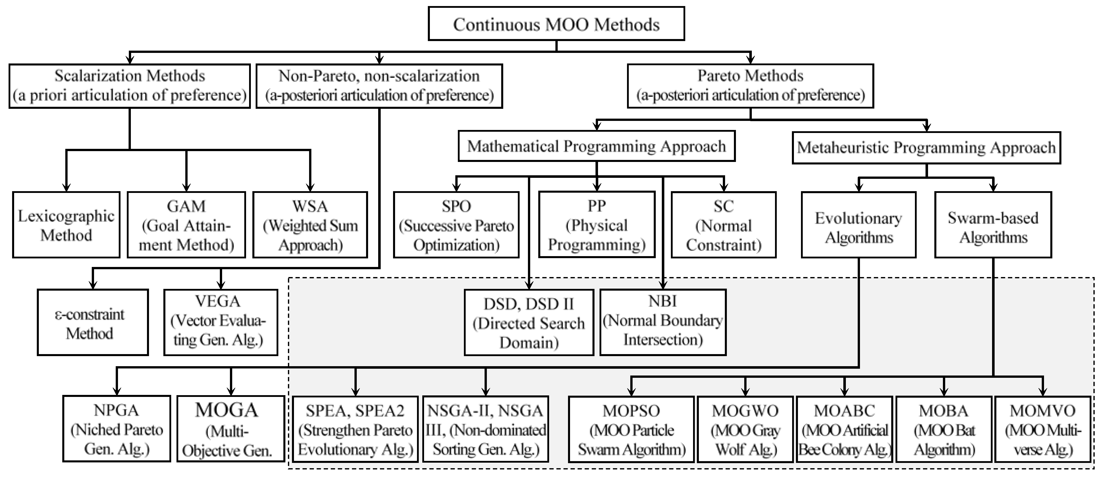
2.2. Methods Founded on the Mathematical Programming

The NBI is one of the first algorithms to compute the Pareto front by using mathematical programming. Later, several algorithms were proposed to improve its performance and to overcome its drawbacks. In such a sense, the Normal Constraint (NC) [27], Physical Programming (PP) [28], Successive Pareto Optimization (SPO) [29], and the Directed Search Domain (DSD) [19] can be cited.

The above-mentioned methods transform the multiobjective problem into many single-objective constrained subproblems. Thus, the optimization is carried out by using a single-objective solver subjected to imposed restrictions. The standard solver is the active-set algorithm, which works reasonably well if the objective functions are smooth and well scaled. These approaches produce a Pareto front with equally spaced points within the framework of a fast convergence, which are important properties for control applications.

2.3. Methods Founded on the Metaheuristic Programming

The methods based on metaheuristic programming can be grouped into evolutionary algorithms and particle swarm intelligence. Multiobjective evolutionary algorithms (MOEA) define first an initial set of solutions (initial population) and then attempt to refine the set of solutions by means of a random selection from the solution space until the optimal Pareto set is obtained.

The population is renewed by the action of several genetic operators, which are known as recombination (a new point is generated from the other point of the population, e.g., averaging), mutation (a recently created point is randomly chosen and replaced with another obtained via the realization of a random variable) and selection (newly created points are taken from the new population considering the best fitness and used to replace points from the old population). These three operations are implemented by many different evolutionary algorithms (for a comparative study, see [30]).

Particle swarm optimization is another stochastic optimization method. It starts with an initial population of particles, which evolve and survive until the last generation. This characteristic distinguishes particle swarm intelligence from evolutionary algorithms, where the population changes.

Particle swarm algorithms search the space of variables by using knowledge from old generations and going at a specifically determined speed within the direction of the global best particle. Many other algorithms were created following this principle. The common idea is to imitate the behavior of various swarms or colonies of animals, such as bats, bees, or ants. However, it should be distinguished from algorithms like MOALO and MOGWO, which emulate the hunting activities of antlions and grey wolves and their interaction with prays. These are based on the Predator-Prey formalism [31].

2.4. Methods for Bilevel Multiobjective Optimization Problems

Bilevel multiobjective optimization consists of two multiobjective optimization algorithms running at two different levels, where one algorithm runs inside the other one. The internal algorithm solves the low-level optimization problem while the external algorithm processes the upper-level problem. This is a nested operation, where the outer algorithm calls the inner one at every upper-level point. Hence, the computational burden of the bilevel optimization algorithm is very high and, therefore, it can only be used by applications that require optimization of low complexity. It is common to find metaheuristic programming at the external level and mathematical programming at the internal one. Nonetheless, both levels can be satisfied for the same class of algorithms. This optimization concept is not considered in the current study, but it is an ongoing research topic.

2.5. Selecting Methods for the Application

Optimization algorithms for MOO problems work properly for a limited number of applications [7] and, therefore, it is difficult to suggest one. Thus, recommendations are exceptionally formulated in the literature. As an indication of general purposes, it is pointed out in [32] that methods that guarantee necessary and sufficient conditions for Pareto optimality should be tested first. In the second term, methods with only guaranteed sufficient conditions may be studied, followed at the end by other methods.

From a practical standpoint, having numerous algorithms may be beneficial in terms of being able to select the most appropriate one according to the application. Hence, the designer can prioritize the choice where accuracy of the solution, computational load, regular distribution of Pareto points on the front, and speed of convergence are just a few examples.

3. Objective Functions for MOO Control Problems

Using advanced optimization techniques, the appropriate choice of the objective functions is crucial for an effective control system design. This is particularly relevant in the case of MOO, since several objectives must be compromised at the same time. Moreover, the objective functions must not only be a useful indicator for the operation of the control system, but they also have to fulfill the corresponding mathematical properties imposed by the optimizer.

3.1. Typical Performance Indices

Performance indices are widely used as objective functions in the classic optimization problem of control systems. They are normally expressed in the form of a function of the control error in the form of

$$J={{\displaystyle \int }}_0^{\infty }f[e(t)]dt\mathrm{and}J={\displaystyle \sum _{k=0}^{\infty }f[e(k)]}$$

(3)

for the continuous and discrete time cases, respectively. Function f can be, for instance, $|e(t)|$ (Integrated Absolute value of Error, AIE), $e{(t)}^2$ (Integral Squared Error, ISE), $te{(t)}^2$ (Integral Time-weighted Squared Error, ITSE) and $t^{2}e{(t)}^2$ (Integral Squared Time-weighted Squared Error, ISTSE). Function f can also include an argument for the control error derivative, which acts as a soft constraint for the control error rate, i.e.,

$$J={{\displaystyle \int }}_0^{\infty }f[e(t),\dot{e}(t)]dt\mathrm{and}J={\displaystyle \sum _{k=0}^{\infty }f[e(k),\Delta e(k)]}.$$

(4)

In general, several other variables and their derivatives can be added as soft constraints for control signals to obtain more complex objective functions of the form

$$J={{\displaystyle \int }}_0^{\infty }f[e(t),\dot{e}(t),u(t),\dot{u}(t)]dt\mathrm{and}J={\displaystyle \sum _{k=0}^{\infty }f[e(k),\Delta e(k),u(k),\Delta u(k)]}.$$

(5)

3.2. Performance Indices for Time-Limited Problems

The performance indices of the previous subsection consider infinite time. However, these indices can be solved only in a few cases, where the Laplace transform is used to leave the time domain. However, this is not possible in the case of nonlinear systems. Another procedure is the evaluation of performance indices by using simulation data. In such a case, the time series are truncated and, as a consequence, the integrals must be averaged in time, as for instance,

$$J=\frac{1}{t_{\max }-t_{\min }}{{\displaystyle \int }}_{t_{\min }}^{t_{\max }}f[e(t)]dt\mathrm{and}J=\frac{1}{(N-k_0)T_s}{\displaystyle \sum _{k=k_0}^{N}f[e(k)]}.$$

(6)

T_s is the sampling time. Time-averaged integral can be used for all performance indices proposed in Section 3.1.

3.3. Performance Indices Formulated Using Fractional Order Calculus

Fractional-order analysis was developed in the 19th century as a generalization of integer-order integral-differential calculus to the real-order case. This work was undertaken by several well-known mathematicians, for example, Cauchy, Euler, Grünwald, Letnikov, Liouville, and Riemann [33].

Another application field for the fractional-order calculus is the system theory and control, where many new developments were carried out in the past 15 years (see, among others, [34]). Integral performance indices as described in 3.1 can also be formulated in the framework of the fractional calculus. Thus, it is pointed out in [35] that a control application presents a better response in the case of oscillatory signals when it is designed using a fractional order cost function. An application of MOO control using fractional order performance indices is reported in [36].

Moreover, the classic performance indices presented at the beginning of this section were generalized in [37] for fractional-order integrals. The continuous time performance index (4) is expressed in the sense of the fractional integral by

$$J=\frac{1}{t_{\max }-t_{\min }}{{\displaystyle \int }}_{t_{\min }}^{t_{\max }}{D}^{(1-k)}f[e(t)]dt,$$

(7)

where D^(1−k) is the fractional derivative and k the fractional order.

The fractional definite integral of Equation (7) can be solved by means of the fractional Barrow formula if an admissible fractional derivative such as the Grünwald–Letnikov or Liouville formula is used [38]. The implementation of the fractional integral can be done by using, for instance, N-Integer [39] or FOTF [40].

3.4. Objective Functions for Specific Applications

In the case of control system design, time domain specifications like maximum rise time, minimum settling time, and minimum overshoot or frequency domain specifications like bandwidth, gain margin, phase margin, and resonant peak can be used as metrics for MOO control. However, since such measures are not convex, MOO algorithms can fail during the optimization process. The construction of solid and mathematically sound objective functions based on the above-mentioned metrics for MOO control is still an open subject.

Following this idea, a convex objective function including fatigue damage was proposed in [41] for the particular cases of wind turbine control. The metric is designed to formulate a compromise between the pitch actuation and the reduction of blade fatigue produced by the individual pitch control.

Wind turbine systems are also characterized by periodic signals as a consequence of the permanent rotation. Hence, the use of such variables in the objective functions is difficult because integrals do not converge. A possible way to overcome the limitation is to evaluate the functions in a finite period or to construct a piecewise signal for the objective function that considers only some periods of the original signal and zero for the rest. This procedure is often used to build an objective function including three 120-degree shifted coupled moments (M₁, M₂, M₃). The cost function is then defined as

$$J=(1/3)\sqrt{M_1^2+M_2^2+M_3^2}.$$

(8)

4. Evaluation of Objective Functions

The evaluation of the objective functions is carried out by the solver several times per iteration during the numerical optimization process. This evaluation means, for example, the calculation of the definite integrals (3–5). The values of the objective functions can be computed in two different ways: the evaluation based on models and the evaluation based on simulation data. Both are explained in the following.

4.1. Evaluation of Objective Functions Based on Dynamic Models

Objective functions are normally related to output variables of a system, whose behavior is represented by a dynamic model. If the model is linear and the objective function is simple, it is possible to find a closed formula to compute the objective function. In the case of [42], models are given in the form of transfer functions, and the infinite integrals (3)–(5) are computed using the Parseval formula

$$J={{\displaystyle \int }}_0^{\infty }f(t)g(t)dt=\frac{1}{2\pi j}{{\displaystyle \int }}_{-j\infty }^{j\infty }F(s)G(-s)ds,$$

(9)

(or its discrete-time counterparts) combined with the Åström–Jury–Agniel algorithms [43]. This approach is also used here in the numerical study. The study case in Section 6 demonstrates how to use this formula from a practical point of view.

4.2. Evaluation Based on Simulation Data

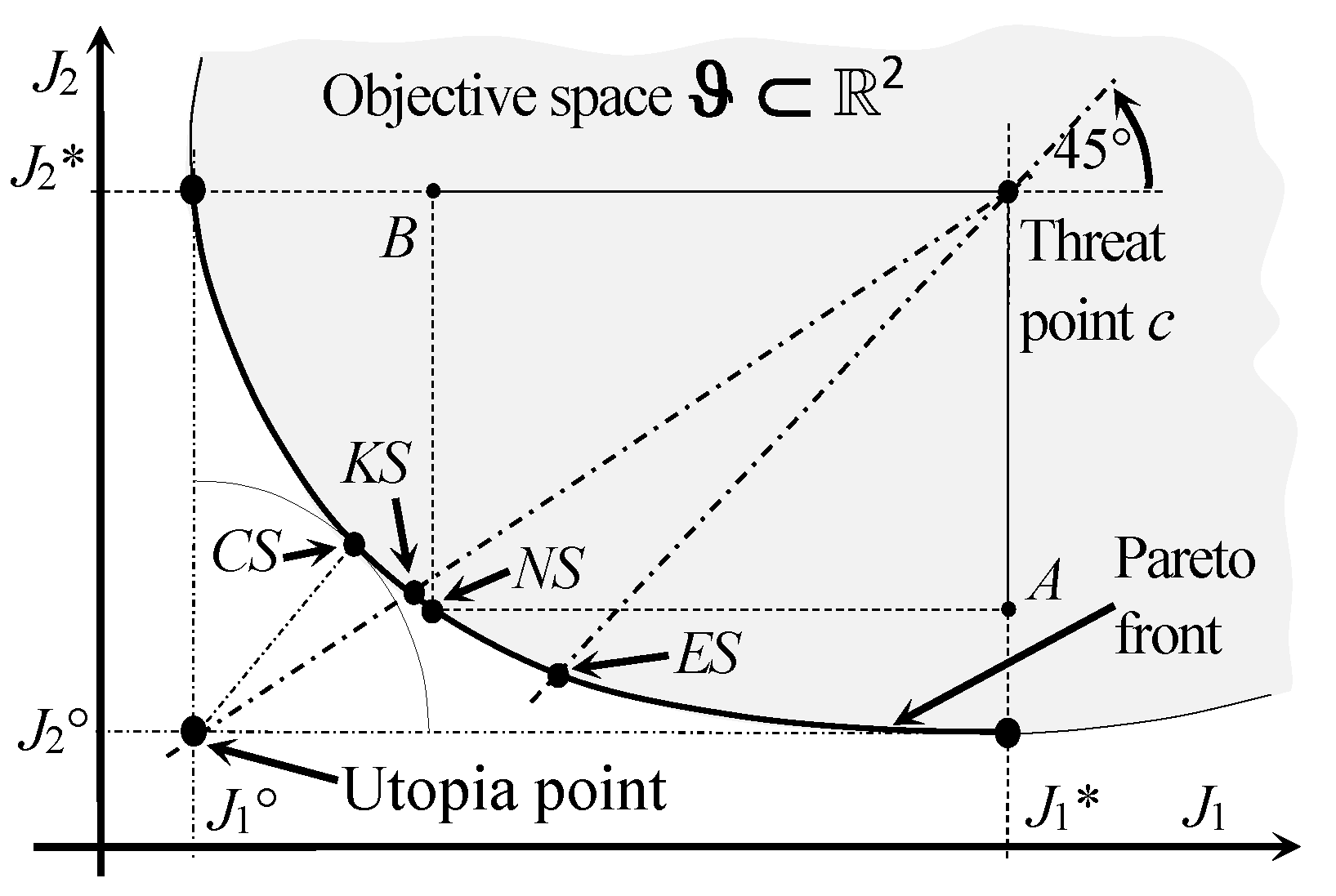
As previously seen, the evaluation based on models is restricted to linear systems with specific objective functions. However, the approach cannot be used in the case of highly complex objective functions. Fractional order objective functions present a similar difficulty because an extension of the Parseval formula for fractional integrals and a numerical procedure to compute them are still unavailable at present. An alternative methodology is to compute the objective functions numerically as part of the simulation.

The benefit of this approach is that almost every type of objective function can be computed. The disadvantage is that simulations must be ended at a finite point in time, and consequently, steady-state values can only be obtained by approximation. In such a situation, time-averaged objective functions (see Section 3.2) should be applied.

Another weakness of the simulation-based approach is the need for long simulation times. It is remarked in [44] that the numerical evaluation of objective functions by using simulation data may take from minutes to days. Practical experience shows that a fast MOPSO algorithm requires about 45 days to generate a three-dimensional Pareto surface in a control design problem, including three objective functions and a simulation time of 60 s. The simulation-based approach is schematized in Figure 3.

5. Decision-Making

All points of the Pareto front are equally optimal and valid solutions to the vector optimization problem. Although all points can be selected for final control implementation, not all points provide the same performance. Hence, the final solution is carried out by a decision maker. Two main concepts can be applied to decision-making. The first one is to introduce additional criteria, as, for example, particular specifications for the closed loop control system design, and the other one is to establish a point in the Pareto front that represents a good balance for all objective functions.

5.1. Approach Using Additional Control Criteria

The idea here is to introduce a second optimization round with search space in the optimal Pareto set and a particular control system specification that has to be satisfied as an objective function (for instance, minimum overshoot, minimum settling time, maximum bandwidth, etc.). For example, the minimum structured singular value is used in [45] to select the controller with the best robustness contained within the Pareto set.

This second round only selects the best possibility as an additional feature for the analyzed property inside the finite Pareto set. Therefore, the solution is normally suboptimal with regard to an optimal solution obtained for this property as a direct optimization in the first round.

5.2. Approach Using a Compromise between the Criteria

This approach does not require evaluation of supplementary objective functions to select the solution. This technique can be implemented by means of cooperative negotiation [46] or bargaining games [47]. The latter is a helpful and simple mechanism that is explained in the following.

Beginning with the shortest distance between the utopia point and the Pareto front, which is known as the compromise solution (CS), bargaining games offer various possible solutions. The shortest distance is computed from

$$J_{CS}=\arg \underset{i}{\min }\left[\sqrt{{\displaystyle {\sum }_{j=1}^n{(J_{ji}-J_j^{°})}^2}}\right].$$

(10)

The Nash bargaining game provides the solution (NS) as the point on the Pareto front that maximizes the n-volume

$$J_{NS}=\arg \underset{i}{\max }\left[{\displaystyle {\prod }_{j=1}^n(J_{ji}-J_j^{°})}\right].$$

(11)

In the case of a two-dimensional problem, it is the area of the rectangle (c, B, NS, A) in Figure 4. The Kalai–Smorodinsky solution (KS) to the game is formally expressed as

$$J_{KS}=\mathrm{maximal}\mathrm{point}\mathrm{of}J\mathrm{on}\mathrm{the}\mathrm{segment}\mathrm{connecting}(J_1^{\ast },J_2^{\ast },\cdots ,J_n^{\ast }\left)\mathrm{to}\right(J_1^{°},J_2^{°},\cdots ,J_n^{°}).$$

(12)

The Kalai–Smorodinsky solution is defined geometrically as the intersection point between the straight line connecting the threat point to the utopia point and the Pareto front for two-dimensional problems. Finally, the Egalitarian solution is defined by

$$J_{ES}=\mathrm{maximal}\mathrm{point}\mathrm{in}J\mathrm{for}\mathrm{which}{J}_i-J_i^{\ast }=J_j-J_j^{\ast },i,j=1,\cdots ,n,$$

(13)

which becomes the intersection point between the Pareto front and a 45°-ray passing through the threat point if the problem includes only two dimensions. All cases of two objective functions are illustrated in Figure 4.

6. Application Study

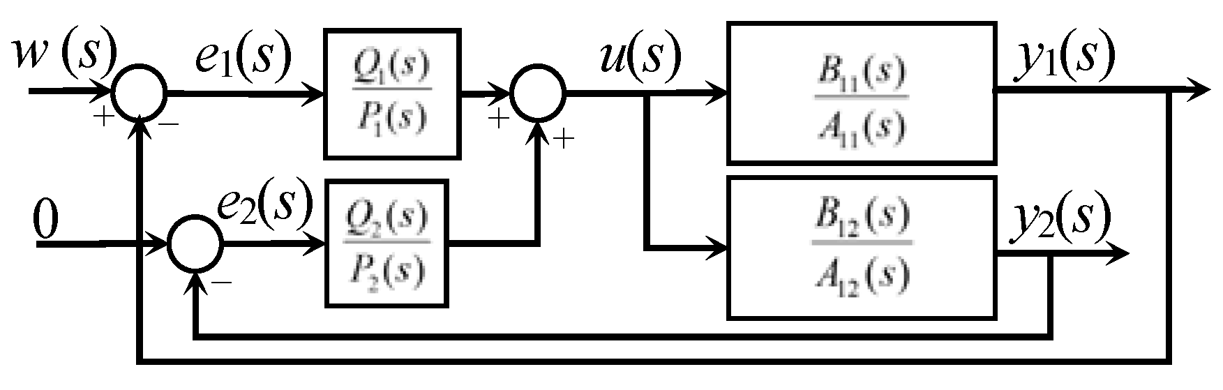
6.1. Description of the Application and the Control Problem

A numerical example of the wind turbine control systems is introduced in the following to study the behavior of the multiobjective optimization algorithms. The application is the generator speed control of a wind turbine operated in the case of overrated wind speed. The control variable is the blade pitch angle acting through the pitch actuator. A characteristic of this control system is the fact that the pitching activity introduces disturbances to the tower and, consequently, the fatigue increases.

Thus, the control objective is to maintain a constant rotational speed independently of variations in the overrated wind speed and, at the same time, to increase the tower damping to reduce the amplitude of oscillations. The control system, as presented in [48,49], includes two control loops, namely the collective pitch control and the active tower damping control. The control system configuration is presented in Figure 5, where y₁, y₂ and w are the rotational speed of the generator, the fore-aft tower-top acceleration and the rated rotational speed of the generator, respectively.

Both control loops have the same control variable, and therefore, the coupling between control loops is evident. Transfer functions from control errors to the references are described by

$$e_1(s)=\frac{N_1(s)}{D_1(s)}=\frac{P_1[A_{11}(A_{21}{P}_2+B_{21}{Q}_2)r_1-B_{11}{A}_{21}{Q}_2{r}_2]}{(A_{11}{P}_1+B_{11}{Q}_1)(A_{21}{P}_2+B_{21}{Q}_2)-B_{11}{B}_{21}{Q}_1{Q}_2}\mathrm{and}$$

(14)

$$e_2(s)=\frac{N_2(s)}{D_2(s)}=\frac{P_2[-B_{21}{A}_{11}{Q}_1{r}_1+A_{21}(A_{11}{P}_1+B_{11}{Q}_1)r_2]}{(A_{11}{P}_1+B_{11}{Q}_1)(A_{21}{P}_2+B_{21}{Q}_2)-B_{11}{B}_{21}{Q}_1{Q}_2},$$

(15)

respectively, where the Laplace variable s is removed for simplicity. The interdependence between both control loops is also observable from (14) and (15), where both controllers appear in the transfer functions. An important problem at the beginning of the controller tuning occurs when there is no information available to start the search for parameters and there is no reference to the interdependence between them. Hence, an automatic search to find an adequate starting reference is useful. Consequently, a combined search for the optimal parameters of both controllers is an illustrative application to assess Pareto optimization algorithms.

6.2. Simplified Model of the System

The model-based approach is used in the study for the evaluation of the objective functions. Hence, a dynamic model of the wind turbine is necessary. However, the wind turbine is a very complex system, and therefore a simplified model including the rotational dynamics of the powertrain and the fore-aft dynamics of the tower is considered. The state-space equations are given by

$$\begin{array}{l}{\dot{x}}_1=-\frac{D_{dt}}{J_r}{x}_1+\frac{D_{dt}}{J_r}{x}_2-\frac{K_{dt}}{J_r}{x}_3+\frac{1}{J_r}{T}_a(\beta ),\\ {\dot{x}}_2=\frac{D_{dt}}{n_x{J}_g}{x}_1-\frac{D_{dt}}{n_x^2{J}_g}{x}_2+\frac{K_{dt}}{n_x{J}_g}{x}_3-\frac{1}{J_g}{T}_g(x_2),\\ {\dot{x}}_3=x_1-\frac{1}{n_x}{x}_2,\\ {\dot{x}}_4=x_5,\mathrm{and}\\ {\dot{x}}_5=-\frac{K_t}{m_t}{x}_4-\frac{D_t}{m_t}{x}_3+\frac{1}{m_t}{F}_t(\beta ),\end{array}$$

(16)

where x₁ = ω_r, x₂ = ω_g, x₃ = θ_r − n_x θ_g, x₄ =x_t, and $x_5={\dot{x}}_t$. Moreover, m, J, K, D, and n_x are mass, mass second moments of inertia, stiffness coefficients, damping coefficients, and the gearbox ratio. Furthermore, θ, ω, F, T and β are variables, which denote rotation angle, rotation speed, force torque, and pitch angle, respectively. T_a, T_g and F_t are the inputs and ω_g and ${\dot{x}}_t$, the outputs. The lowercase letters dt, r, g, a, t and x represent the subscripts used to describe the drivetrain, rotor, generator, aerodynamic, tower, and gearbox, respectively.

Parameters for the model (16) are obtained from the reference wind turbine proposed in [50], which was analyzed in [51] from the control perspective. The most important parameters are summarized in

Table 1. Essential model parameters.

Parameter	Variable	Values	Units
Rated power	P0	20 × 106	W
Rated rotor speed	ωr0	0.7494	rad/s
Rotor mass moment of inertia	Jr	2919659264.0	kg m2
Generator mass moment of inertia	Jg	7248.32	kg m2
Equivalent shaft damping	Ddt	4.97 × 107	Nm/rad
Equivalent shaft stiffness	Kdt	6.94 × 109	Nm/(rad/s)
Damping ratio of the drivetrain	ζdt	5	%
Mass of tower	mt	1782947.0	kg
First in-plane blade frequency	ft	0.1561	Hz
Damping ratio of the tower	ζt	5	%
Equivalent tower stiffness	Kt	4 π2 ft2 mt	Nm/(m/s)
Equivalent tower damping	Dt	$2{\zeta }_t\sqrt{m_t{K}_t}$	Nm/rad
Gearbox ratio	nx	164	--
Generator efficiency	ηg	94.4	%

© [2020] IEEE. Reprinted, with permission, from [10].

.

Since the inputs of (16) are nonlinear, they are linearized about an operating point for an effective wind speed of 11.4 m/s, which corresponds to a pitch angle of β₀ = 3.620 deg and a rotational speed of 7.15 rpm. Under such conditions, the inputs become

$$T_a\approx \frac{P_0}{{\omega }_{r0}}+\frac{1}{{\omega }_{r0}}{\frac{\partial P}{\partial \beta }|}_{{\beta }_0}\Delta \beta ,T_g\approx \frac{P_0}{n_x{\omega }_{r0}}-\frac{P_0}{n_x^2{\omega }_{r0}^2}\Delta {\omega }_g\mathrm{and}{F}_t\approx F_{t0}+{\frac{\partial F_t}{\partial \beta }|}_{{\beta }_0}\Delta \beta ,$$

(17)

where Δβ = β − β₀, Δω = ω − ω₀, $\partial P/\partial \beta |{\beta }_0=-2.10567\times {10}^8$, $\partial F_t/\partial \beta |{\beta }_0=-2.3073\times {10}^7$ and $P_0/n_x^2{\omega }_{r0}^2=-2.3\times {10}^5$. For the pitch actuators, a first order dynamics with a time constant of T_a = 0.2 s is assumed. Finally, the transfer functions with reduced orders according to Figure 5, model (16) and Table 1 are

$$G_{11}(s)=\frac{B_{11}(s)}{A_{11}(s)}=\frac{-(20.1s+2809.1)}{s^4+5.272s^3+38.6281s^2+87.5669s-493.8741}\mathrm{and}$$

(18)

$$G_{12}(s)=\frac{B_{12}(s)}{A_{12}(s)}=\frac{-64.7056s}{s^3+5.0981s^2+1.45246281s+4.8099}.$$

(19)

respectively. The collective pitch control loop is implemented by means of a PID controller and the active tower damping control by a P controller, whose polynomials are P₁(s) = 1/s, P₂ = 1, Q₁(s) = q₀ s² + q₁ s + q₂ and Q₂ = K. The parameter vector α, which has to be found by the MOO algorithms, is consequently α = (q₀ q₁ q₂ K).

It is pointed out in [52] that the ISE performance index often exhibits oscillatory behavior as a consequence of the large errors occurring at low time intervals, which contribute significantly to the performance index. This disadvantage is avoided here by using a time-weighted ISE performance index (ITSE) defined by

$$J_{ITSE}={{\displaystyle \int }}_0^{\infty }te{(t)}^{2}dt.$$

(20)

6.3. Mechanization of the Optimization Procedure

The first step is to generate an objective function that can be evaluated by the MOO algorithms. From the general Parseval Formula (9) and the ITSE index (20), functions f(t) and g(t) can be defined as

$$f(t)=e(t)\mathrm{and}g(t)=te(t),$$

(21)

respectively. According to (14) and (15), the Laplace transform of f(t) can be described by a polynomial rational function, i.e.,

$$F(s)=e(s)=\frac{N(s)}{D(s)}$$

(22)

and the Laplace transform of g(t) is

$$G(s)=-\frac{de(s)}{ds}=-\frac{dF(s)}{ds},$$

(23)

which can also be expressed as the polynomial rational function

$$G(s)=-\frac{(dN/ds)D-N(dD/ds)}{D{(s)}^2}.$$

(24)

The derivatives are then obtained by polynomial differentiation, that is,

$$dD(s)/ds=n_d{d}_0{s}^{n_d-1}+(n_d-1)d_1{s}^{n_d-2}+\cdots +2d_{n_d-2}s+d_{{}^{n_d-1}}\mathrm{and}$$

(25)

$$dN(s)/ds=n_n{n}_0{s}^{n_n-1}+(n_n-1)n_1{s}^{n_n-2}+\cdots +2n_{n_n-2}s+n_{n_n-1}.$$

(26)

If the functions F and G are rational, i.e.,

$$J=\frac{1}{2\pi j}{\int }_{-j\infty }^{j\infty }\frac{B_1(s)}{A_1(s)}\frac{C_1(-s)}{A_1(-s)}ds.$$

(27)

the complex integral of Equation (16) can be solved using the Åström–Jury–Agniel algorithm [43] modified by [53]. Hence, the evaluation of the objective functions is completed, defining

$$A_1(s)=D{(s)}^2,B_1(s)=D(s)N(s)\mathrm{and}$$

(28)

$$C_1(s)=N(s)[dD(s)/ds]-D(s)[dN(s)/ds],$$

(29)

where N and D are either N₁ and D₁ from (14) for the first control loop or N₂ and D₂ from (15) for the second control loop. A Matlab implementation of the generalized algorithm to compute (27) can be found in [42].

It is important to remark that the condition for the existence of the solution is that polynomials D₁ and D₂ are stable, which is satisfied by the controller design. Thus, closed-loop stability is checked for every choice of controller parameters in the search space during the optimization process.

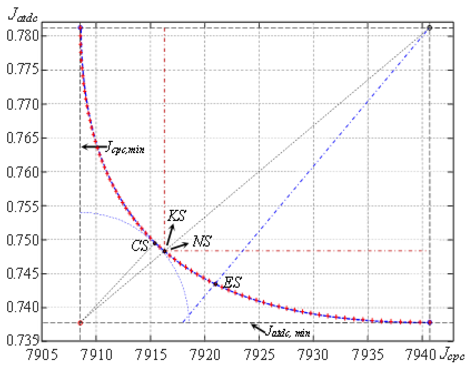
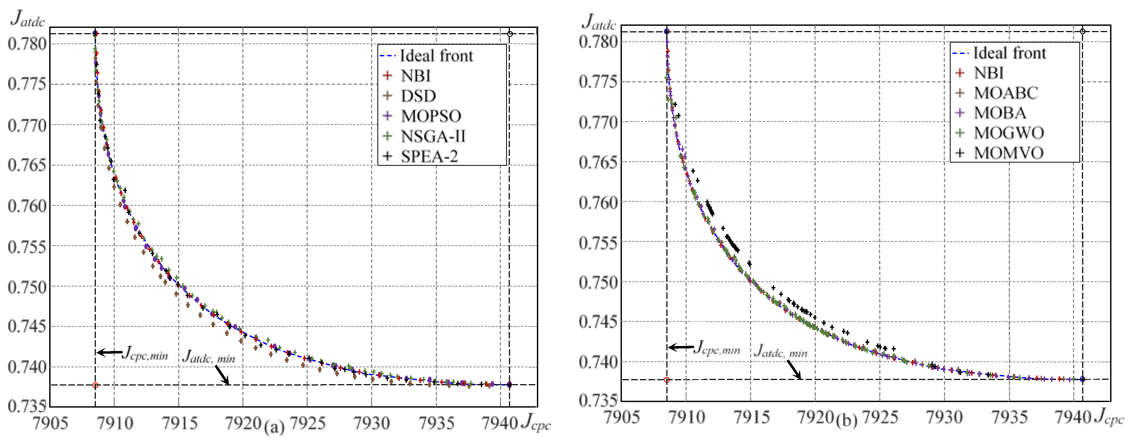
7. Optimization Results

To carry out a quantitative assessment of the optimization outcomes, the effective computation time for a whole Pareto front of 70 points, the number of evaluations of the objective functions during the optimization process, the inverted generational distance (IGD), the spread (SP), and epsilon ε (see [54,55]) are considered.

7.1. Evaluation Procedure for the MOO Algorithms

The computational burden of the algorithms is obtained by time measurement of the complete optimization run. The final numbers correspond to the average of ten runs for each algorithm. In addition, the required number of evaluations of the objective functions is included in the assessment.

Several other indicators for the quality of the obtained Pareto front are considered. The Inverted Generational Distance (IGD, [56]) is an indicator of the Euclidean distance between the computed and the true Pareto fronts, which is considered a reference. The IGD is computed by using the Euclidean distance d for each point of the Pareto front according to equation $IGD=(1/n)({{\sum }_{i=1}^n{d}_i^2)}^{0.5}$ for n as the total number of points in the Pareto front. When the IGD is equal to zero, the computed Pareto front is equal to a real one. The spread [57], also known as distribution, is computed as $SP=({\sum }_{i=1}^n\max {(||J_{i,\max }-J_{i,\min }||)}^{0.5}$, where J_i,max and J_i,min are the individual maximum and minimum values of the ith objective function. Lower values indicate better coverage. Lastly, epsilon determines if one estimation set is worse than another. In the current work, the real Pareto front is compared with the results of all algorithms. As a result, a lower value for one algorithm implies that it is a better estimation than the other.

7.2. Assessment of Results

The optimization results are only true for the application under consideration and cannot be assumed to be generally valid. The results provided by the metrics are shown in

Table 2. Summary of values provided by indicators on optimization algorithms.

Algorithm	Time [s]	Evaluations	IGD	SP	Epsilon
DSD	3.2080	1200	0.1420	0.0531	0.0048
MOABC	14.7438	20243	0.0349	0.0137	2.7589 × 10−4
MOBA	6.9250	14070	0.0097	0.0031	2.0520 × 10−4
MOGWO	7.0332	14070	0.0562	0.0170	2.2919 × 10−4
MOMVO	11.0681	40000	0.1444	0.0146	1.3056 × 10−4
MOPSO	4.4882	14280	0.0196	0.0064	7.5852 × 10−5
NBI	1.9437	4134	0.0077	0.0025	6.8926 × 10−5
NSGA-II	2.9186	1200	0.0175	0.0056	3.1163 × 10−4
SPEA-2	4.6237	14000	0.0108	0.0036	3.4632 × 10−6

© [2020] IEEE. Reprinted, with permission, from [10].

. The best values are emphasized in bold and italic, and the second-best values in bold. Overall, NBI, as well as NSGA-II and MOPSO, appear to be good options for these types of control problems. It is interesting to analyze the results produced by MOBA. It belongs to the swarm intelligence-based algorithms, which is a group whose performance can be placed in a second position. However, the numbers produced by MOBA are closer to those of the first category.

Figure 6 depicts the outcomes produced by the decision maker based on bargaining games for the Pareto front created by NBI. The regularly distributed Pareto front, which is a characteristic of NBI, simplifies the solution finding process. At long last, Figure 7 shows the Pareto fronts obtained from all studied algorithms.

7.3. Important Issues Emerging from Practical Experience

Several issues associated with MOO control have come to light during the implementation process that ought to be addressed. For example, there is today a tendency toward using a large number of basic objective functions. Despite evidence that the performance of MOO algorithms for more than two objective functions has improved significantly in recent years, optimization times for problems with three objective functions in the order of hours or days suggest that the effort is still insufficient. Furthermore, decisions-making in such situations becomes a difficult task.

Thus, it is still preferable from the practical point of view to scale down the problem to two complex objective functions, clustering multiple basic objectives into two classes. This idea can be realized by using the concept of cooperative and non-cooperative team games combined with a weighted sum objective function per team, where each summed objective function includes a collection of noncontradictory characteristics. As a result, conflicting criteria are assigned to different teams.

Another open aspect is the initialization of the algorithms by setting start values. Depending on these values, convergence usually takes more or less time. At present, there are no optimal and automatic procedures to initiate the algorithms, and therefore, experience is necessary to minimize the time for trial and error. In particular, algorithms need a search space at the start, which is typically not free in numerous control problems. For instance, if the stability region for the controller parameters is unknown a priori and the search ranges for the parameters are chosen incorrectly, the closed-loop system may become unstable at start, and the algorithm will take a long time to converge to a stability region. It is also possible that the whole optimization takes places outside the parameter stabilizing region and the optimization becomes infeasible. Thus, previous work should be to determine first the stabilizing parameter region to define the start search range inside it.

Related to the previously described issue is the fact that there are often several unconnected stabilizing search spaces. Since MOO algorithms are restricted to work within a fixed search space, the global optimum could never be reached because the corresponding parameters are in a different search space. Furthermore, the value of one parameter often extends or contracts the stability range of other parameters, causing the effect that the search spaces of other parameters change all the time. This effect is illustrated in Figure 8, where it can be observed that the search space for (q₀ q₁ q₂) depends on the value of parameter p₁.

All these cases are not considered in the existing MOO algorithms. Thus, algorithms with variable, conditioned, and discontinuous search ranges are needed, but they are currently unavailable.

Finally, current MOO algorithms are not deterministic in the computer science sense. Therefore, there is no guarantee that MOO control approaches can work in a real-time environment where the optimization must be finished inside a sampling period to meet the deadlines.

8. Conclusions

In this paper, multiobjective optimal (MOO) control is investigated from the user perspective. Multiobjective optimization is introduced shortly. In particular, aspects related to the control application, such as, for example, the selection and evaluation of objective functions as well as the decision-making process, are examined. Several old and relatively new MOO algorithms are studied from the control viewpoint by using an example from wind energy control systems. The performances of the algorithms are compared quantitatively by using standard indicators for MOO algorithms.

Results show that old-stablished algorithms like NBI, NSGA-II, and MOPSO are solid and still maintain the state of the art, at least for control applications. From the latest algorithms, MOBA stands out, but in general, they all need to be improved for real-life control applications. In addition, several aspects arising from user experience were reported and limitations regarding the stability of the closed loop system and search spaces are highlighted.

In general, multiobjective optimization is a sophisticated tool that greatly aids in the effort to master the control system design of very complex applications. On the other hand, the current state of the art of MOO algorithms only allows a limited use.

Finally, the work is focused on the comparison of MOO methods for solving multiple control loops with multiple controllers and the associated problems. Since all methods solve the same objective functions with the same parameters, it is also expected that they provide the same results for the same decision-making. Thus, a study of the parametric sensibility and robustness of results is necessary before concluding whether the methods can be thrust for application with real wind turbines in real-time operation. Such aspects are currently being analyzed and will be reported in a future work.

References

1. Liu, G.P.; Yang, J.B.; Whidborne, J.F. Multiobjective Optimisation and Control; Research Studies Press Ltd.: Exeter, UK, 2003. [Google Scholar]
2. Gambier, A.; Badreddin, E. Multi-objective optimal control: An overview. In Proceedings of the IEEE Conference on Control Applications, Singapore, 1–3 October 2007; pp. 170–175. [Google Scholar]
3. Gambier, A. MPC and PID control based on multi-objective optimization. In Proceedings of the 2008 American Control Conference, Seattle, WA, USA, 11–13 June 2008; pp. 2886–2891. [Google Scholar]
4. Gambier, A.; Jipp, M. Multi-objective optimal control: An introduction. In Proceedings of the Asian Control Conference, Kaohsiung, Taiwan, 15–18 May 2011; pp. 1084–1089. [Google Scholar]
5. Reynoso-Meza, G.; Ferragud, X.B.; Saez, J.S.; Durá, J.M.H. Controller Tuning with Evolutionary Multiobjective Optimization: A Holistic Multiobjective Optimization Design Procedure, 1st ed.; Springer: Cham, Switzerland, 2017. [Google Scholar]
6. Peitz, S.; Dellnitz, M. A survey of recent trends in multiobjective optimal control—Surrogate models, feedback control and objective reduction. Math. Comput. Appl. 2018, 23, 30. [Google Scholar] [CrossRef] [Green Version]
7. Wolpert, D.H.; Macready, W.G. No free lunch theorems for optimization. IEEE Trans. Evol. Comput. 1997, 1, 67–82. [Google Scholar] [CrossRef] [Green Version]
8. Eichfelder, G. Multiobjective bilevel optimization. Math. Program. 2010, 123, 419–449. [Google Scholar] [CrossRef]
9. Liang, J.Z.; Miikkulainen, R. Evolutionary bilevel optimization for complex control tasks. In Proceedings of the 2015 Annual Conference on Genetic and Evolutionary Computation, Madrid, Spain, 11–15 July 2015; pp. 871–878. [Google Scholar]
10. Gambier, A. Multiobjective Optimal Control: Algorithms, Approaches and Advice for the Application. In Proceedings of the 2020 International Automatic Control Conference, Hsinchu, Taiwan, 4–7 November 2020; pp. 1–7. [Google Scholar]
11. Pareto, V. Manuale di Economia Politica; Societa Editrice Libraria: Milan, Italy, 1906; (Translated into English by A. S. Schwier as Manual of Political Economy, Macmillan, New York, 1971). [Google Scholar]
12. Miettinen, K.M. Nonlinear Multiobjective Optimization, 4th ed.; Kluwer Academic Publishers: New York, NY, USA, 2004. [Google Scholar]
13. de Weck, O.L. Multiobjective optimization: History and promise. In Proceedings of the 3rd China-Japan-Korea Joint Symposium on Optimization of Structural and Mechanical Systems, Kanazawa, Japan, 30 October–2 November 2004; pp. 1–14. [Google Scholar]
14. Das, I.; Dennis, J.E. Normal-Boundary Intersection: A new method for generating the Pareto surface in nonlinear multicriteria optimization problems. SIAM J. Optim. 1998, 8, 631–657. [Google Scholar] [CrossRef] [Green Version]
15. Deb, K.; Pratap, A.; Agarwal, S.; Meyarivan, T. A fast and elitist multiobjective genetic algorithm: NSGA-II. IEEE Trans. Evol. Comput. 2002, 6, 182–197. [Google Scholar] [CrossRef] [Green Version]
16. Coello, C.A.; Lechuga, M.S. MOPSO: A proposal for multiple objective particle swarm optimization. In Proceedings of the 2002 Congress on the Evolutionary Computation, Honolulu, HI, USA, 12–17 May 2002; pp. 1051–1056. [Google Scholar]
17. Zitzler, E.; Laumanns, M.; Thiele, L. SPEA2: Improving the Strength Pareto Evolutionary Algorithm; Research Report; Swiss Federal Institute of Technology (ETH): Zurich, Switzerland, 2001. [Google Scholar]
18. Motta, R.S.; Afonso, S.M.; Lyra, P.R. A modified NBI and NC method for the solution of N-multiobjective optimization problems. Struct. Multidiscip. Optim. 2012, 46, 239–259. [Google Scholar] [CrossRef]
19. Erfani, T.; Utyuzhnikov, S.V. Directed Search Domain: A Method for even generation of Pareto frontier in multiobjective optimization. J. Eng. Optim. 2010, 43, 1–17. [Google Scholar] [CrossRef]
20. Angus, D.; Woodward, C. Multiple objective ant colony optimisation. Swarm Intell. 2009, 3, 69–85. [Google Scholar] [CrossRef]
21. Akbari, R.; Hedayatzadeh, R.; Ziarati, K.; Hassanizadeh, B. A multi-objective artificial bee colony algorithm. Swarm Evol. Comput. 2012, 2, 39–52. [Google Scholar] [CrossRef]
22. Yang, X.S. Bat algorithm for multi-objective optimisation. Int. J. Bio-Inspired Comput. 2011, 3, 267–274. [Google Scholar] [CrossRef]
23. Deb, K.; Jain, H. An evolutionary many-objective optimization algorithm using reference-point-based nondominated sorting approach, Part I: Solving problems with Box constraints. IEEE Trans. Evol. Comput. 2014, 18, 577–601. [Google Scholar] [CrossRef]
24. Mirjalili, S.; Saremi, S.; Mirjalili, S.M.; Coelho, L.d.S. Multi-objective grey wolf optimizer: A novel algorithm for multicriterion optimization. Expert Syst. Appl. 2016, 47, 106–119. [Google Scholar] [CrossRef]
25. Mirjalili, S.; Jangir, P.; Mirjalili, S.Z.; Saremi, S.; Trivedi, I.N. Optimization of problems with multiple objectives using the multi-verse optimization algorithm. Knowl.-Based Syst. 2017, 134, 50–71. [Google Scholar] [CrossRef] [Green Version]
26. Mirjalili, S.; Jangir, P.; Saremi, S. Multi-objective ant lion optimizer: A multi-objective optimization algorithm for solving engineering problems. Appl. Intell. 2017, 46, 79–95. [Google Scholar] [CrossRef]
27. Messac, A.; Mattson, C. Normal constraint method with guarantee of even representation of complete Pareto frontier. AIAA J. 2004, 42, 2101–2111. [Google Scholar] [CrossRef] [Green Version]
28. Messac, A. Physical programming: Effective optimization for computational de sign. AIAA J. 1996, 34, 149–158. [Google Scholar] [CrossRef]
29. Mueller-Gritschneder, D.; Graeb, H.; Schlichtmann, U. A successive approach to compute the bounded Pareto front of practical multiobjective optimization problems. SIAM J. Optim. 2009, 20, 915–934. [Google Scholar] [CrossRef]
30. Kunkle, D. A Summary and Comparison of MOEA Algorithms; Research Report; College of Computer and Information Science Northeastern University: Boston, MA, USA, 2005. [Google Scholar]
31. Grimme, C.; Schmitt, K. Inside a predator-prey model for multiobjective optimization: A second study. In Proceedings of the Genetic and Evolutionary Computation Conference, Seattle, WA, USA, 8–12 July 2006; pp. 707–714. [Google Scholar]
32. Marler, R.T.; Arora, J.S. Survey of multi-objective optimization methods for engineering. Struct. Multidiscip. Optim. 2004, 26, 369–395. [Google Scholar] [CrossRef]
33. Miller, K.S.; Ross, B. An Introduction to the Fractional Calculus and Fractional Differential Equations; John Wiley & Sons: New York, NY, USA, 1993. [Google Scholar]
34. Monje, C.A.; Chen, Y.; Vinagre, B.M.; Xue, D.; Feliu-Batlle, V. Fractional-Order Systems and Controls, 1st ed.; Springer: London, UK, 2010. [Google Scholar]
35. Das, S.; Pan, I.; Halder, K.; Das, S.; Gupta, A. LQR based improved discrete PID controller design via optimum selection of weighting matrices using fractional order integral performance index. Appl. Math. Model. 2013, 37, 4253–4268. [Google Scholar] [CrossRef]
36. Gambier, A. Evolutionary multiobjective optimization with fractional order integral objectives for the pitch control system design of wind turbines. IFAC-PapersOnLine 2019, 52, 274–279. [Google Scholar] [CrossRef]
37. Romero, M.; de Madrid, A.P.; Vinagre, B.M. Arbitrary real-order cost functions for signals and systems. Signal Process. 2011, 91, 372–378. [Google Scholar] [CrossRef]
38. Ortigueira, M.; Machado, J. Fractional definite integral. Fractal Fract. 2017, 1, 2. [Google Scholar] [CrossRef] [Green Version]
39. Valério, D.; Sá da Costa, J. Ninteger: A non-integer control toolbox for MatLab. In Proceedings of the First IFAC Workshop on Fractional Differentiation and Applications, Bordeaux, France, 19–21 July 2004; pp. 208–213. [Google Scholar]
40. Xue, D. FOTF toolbox for fractional-order control systems. In Volume 6 Applications in Control; Petráš, I., Ed.; De Gruyter: Berlin, Germany, 2019; Volume 6, pp. 237–266. [Google Scholar]
41. Alamir, M.; Collet, D.; Di Domenico, D.; Sabiron, G. A fatigue-oriented cost function for optimal individual pitch control of wind turbines. IFAC-PapersOnLine 2020, 52, 12632–12637. [Google Scholar]
42. Gambier, A. Optimal PID controller design using multiobjective normal boundary intersection technique. In Proceedings of the 7th Asian Control Conference, Hong Kong, China, 27–29 August 2009; pp. 1369–1374. [Google Scholar]
43. Åström, K. Introduction to Stochastic Control Theory; Academic Press: London, UK, 1970. [Google Scholar]
44. Akhtar, T.; Shoemaker, C.A. Efficient Multi-Objective Optimization through Population-Based Parallel Surrogate Search; Research Report; National University of Singapore: Singapore, 2019. [Google Scholar]
45. Wellenreuther, A.; Gambier, A.; Badreddin, E. Application of a game-theoretic multi-loop control system design with robust performance. IFAC Proc. Vol. 2008, 41, 10039–10044. [Google Scholar] [CrossRef]
46. Gatti, N.; Amigoni, F. An approximate Pareto optimal cooperative negotiation model for multiple continuous dependent issues. In Proceedings of the 2005 IEEE/WIC/ACM International Conference on Intelligent Agent Technology, Compiègne, France, 19–22 October 2005; pp. 565–571. [Google Scholar]
47. Thomson, W. Cooperative models of bargaining. In Handbook of Game Theory with Economic 2; Aumann, R.J., Hart, S., Eds.; Elsevier: Oxford, UK, 1994; pp. 1237–1284. [Google Scholar]
48. Gambier, A. Simultaneous design of pitch control and active tower damping of a wind turbine by using multi-objective optimization. In Proceedings of the 1st IEEE Conference on Control Technology and Applications, Kohala Coast, HI, USA, 27–30 August 2017; pp. 1679–1684. [Google Scholar]
49. Gambier, A.; Nazaruddin, Y. Collective pitch control with active tower damping of a wind turbine by using a nonlinear PID approach. IFAC–PapersOnLine 2018, 51, 238–243. [Google Scholar] [CrossRef]
50. Ashuri, T.; Martins, J.R.R.; Zaaijer, M.B.; van Kuik, G.A.M.; van Bussel, G.J.W. Aeroservoelastic design definition of a 20 MW common research wind turbine model. Wind Energy 2016, 19, 2071–2087. [Google Scholar] [CrossRef]
51. Gambier, A.; Meng, F. Control system design for a 20 MW reference wind turbine. In Proceedings of the 3rd. IEEE Conference on Control Technology and Application, Hong Kong, China, 19–21 August 2019; pp. 258–263. [Google Scholar]
52. Zhuang, M.; Atherton, D.P. Tuning PID controllers with integral performance criteria. In Proceedings of the IEE Conference on Control 91, Edinburgh, UK, 25–28 March 1991; pp. 481–486. [Google Scholar]
53. Wan, K.C.; Sreeram, V. Solution of bilinear matrix equation using Astrom-Jury-Agniel algorithm. IEE Proc. Part-D Control Theory Appl. 1995, 142, 603–610. [Google Scholar] [CrossRef]
54. Riquelme, N.; von Lücken, C.; Baran, B. Performance metrics in multi-objective optimization. In Proceedings of the 2015 Latin American Computing Conference, Arequipa, Peru, 19–23 October 2015; pp. 1–11. [Google Scholar]
55. Zitzler, E.; Thiele, L.; Laumanns, M.; Fonseca, C.M.; Grunert da Fonseca, V. Performance assessment of multiobjective optimizers: An analysis and review. IEEE Trans. Evol. Comput. 2003, 7, 117–132. [Google Scholar] [CrossRef] [Green Version]
56. Coello Coello, C.A.; Cortés, N. Solving multiobjective optimization problems using an artificial immune system. Genet. Program. Evol. Mach. 2005, 6, 163–190. [Google Scholar] [CrossRef]
57. Zitzler, E.; Deb, K.; Thiele, L. Comparison of multiobjective evolutionary algorithms: Empirical results. Evol. Comput. J. 2000, 8, 125–148. [Google Scholar] [CrossRef] [PubMed] [Green Version]
Figure 1. Schematic description of the multiobjective optimization problem.
Energies 15 00567 g001
Figure 2. Classification of most important multiobjective optimal (MOO) algorithms (algorithms inside doted gray box are included in numerical study). © [2020] IEEE. Reprinted, with permission, from [10].
Energies 15 00567 g002
Figure 3. Scheme for optimization process with simulation-based evaluation of objective functions.
Energies 15 00567 g003
Figure 4. Description of a two-decisional decision maker according to bargaining games.
Energies 15 00567 g004
Figure 5. Generalized representation of closed-loop control system for study case.
Energies 15 00567 g005
Figure 6. Decision-making based on bargaining games for the NBI Pareto front. © [2020] IEEE. Reprinted, with permission, from [10].
Energies 15 00567 g006
Figure 7. Pareto fronts of all algorithms. (a) NBI, DSD, MOPSO, NSGA-II, and SPEA-2. (b) MOABC, MOBA, MOGWO, and MOMVO, where NBI is included as a reference. © [2020] IEEE. Reprinted, with permission, from [10].
Energies 15 00567 g007
Figure 8. Stabilizing subspaces for (q0 q1 q2) in dependence of parameter p1.
Energies 15 00567 g008