Abstract
In this study, the mixing power and the axial and radial velocity distributions were determined for the standard PBT45-6 impeller with inclined blades and for three NACA impellers with airfoil blades. On the basis of the velocity distributions obtained by means of PIV techniques, the pumping efficiency and the size of the secondary circulation for the tested impellers were determined. The next stage was to calculate the efficiency of the impeller operation, in which the comparative criteria were the values of the mixing energy in the form of a dimensional and dimensionless criterion. The lowest mixing energy was obtained for impellers with symmetrical profiled NACA0021 blades, which was 20% lower than the similar mixing energy obtained for the standard PBT45-6 impeller.
1. Introduction
Axial impellers are used, among other things, in processes defined as flow-sensitive operations [1]. They include the homogenization of miscible liquids, preparation of suspensions of a solid in a liquid, or in heat and mass transfer processes. The term “flow sensitive” suggests that the speed of these processes depends on the liquid flow in the entire volume of the mixing tank. Therefore, knowledge of the characteristics of the liquid flow in the mixer is often the starting point for a quantitative description of these operations.
In our previous work [2], it was established that the application of an aerodynamic (airfoil) profile for the propeller blade cross-section reduces the mixing power significantly. Figure 1 presents two of the tested propellers. The use of the NACA4424 airfoil resulted in almost a 25% reduction in mixing power in comparison with the flat cross-section at the same projection area of the blade on a horizontal plane.
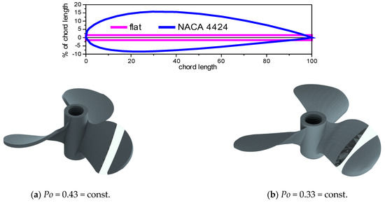
Figure 1.
Propellers and powers numbers. (a) with flat cross-section. (b) with NACA4424 cross-section [2].
However, the reduction in mixing power cannot be the only criterion for assessing the efficiency of new—or only improved—design solutions. The hydrodynamic effects during the operation of the impeller are also important, since they affect the time taken to achieve the required mixing state. In the cited case, to determine the efficiency of the impeller operation, Relationship (1) was used, which determines mixing energy UE that defines how much energy should be supplied to the system in order to obtain good mixing of the liquid appropriate from a technological point of view.
where E—energy required to achieve the assumed mixing degree, J; V—volume of the mixed liquid, m3; P—mixing power, W; 𝜏m—mixing (homogenization) time, s. Relationship (1) defines the mixing efficiency well, but for its determination, it is necessary to know the mixing time 𝜏m needed to achieve the required degree of homogeneity. The mixing time can be associated with the circulation time 𝜏c, which is defined by Equation (2) as the average time needed for each liquid element to make one complete circulation loop in the axial–radial plane.
Information in the literature indicates that three to four circulation loops are required to achieve complete mixing [3,4,5,6,7,8]. This means that the simple Equation (3) can be used to calculate the mixing time 𝜏m.
Information on circulation and homogenization times for individual impellers is most often given on the basis of experimental data [9,10]. However, if there are no literature data for a specific impeller, then Relationship (1) is of little use in determining the efficiency of this impeller. While the average circulation time can be calculated, among things, from the relationship [11,12], the arbitrarily assumed value of the numerical coefficient in Equation (3) may be a source of error. When the exact mixing time is not known, a better efficiency criterion is Relationship (4), based on the dimensionless pumping number Flpump and the power number Po [13].
where Vpump—pumping capacity of the impeller, m3/s; Fl—flow (pumping) number; ρ—density, kg/m3; D—impeller diameter, m; T—tank diameter, m; Po—mixing power number. Pumping capacity Vpump is the value of a liquid stream thrown out by the impeller from its space, i.e., the area specified by the blades of the impeller during its operation. For axial impellers and a known radial profile of axial velocity Uz(r), in the cross-section just below the impeller with radius RM = D/2, the values of Vpump and Flpump will be expressed by the equations
where N—rotational frequency of the impeller, s−1. According to Equation (4), impellers with higher values of Ep are more effective, because for a given mixing power they generate a larger liquid stream.
For the mixing process, the power number is defined by the relationship
During the rotation of the impeller, its blades are subjected to aerodynamic force resulting from two sources:
- Normal force caused by pressure on the body surface;
- Shear force due to fluid viscosity, often referred to as skin friction.
The resultant aerodynamic force acting on the body is equal to the forces due to pressure and the sum of shear forces acting over the entire body surface. This aerodynamic force is usually broken down into two components (both components pass through the center of pressure):
- Drag force, i.e., the component of the force parallel to the direction of rotation of the impeller blade (depending on the resistance coefficient Cd);
- Lifting force, i.e., the component of the force perpendicular to the direction of rotation of the impeller blade (depending on the coefficient of the lifting force Cl).
It can be shown that the mixing power number Po depends on the blade drag coefficient Cd [14], assuming that , , (F—force, N).
That is, the drag coefficient of the impeller Cd and the power number Po are directly proportional. The above description is simplified, because when the impeller rotates, induced drag is also created. It is generated by the circulation of fluid around the rotor blade, which creates lift. For a blade pitch of 45° and flow completely stalled at the airfoil pressure surface, shape drag is likely to have a greater effect on torque and, consequently, on the mixing power (large projection of airfoil area on the r–z plane). During the experimental determination of the torque, its value is influenced by both the shape drag and the induced drag. However, for an accurate theoretical description of the phenomenon, induced resistance should also be taken into account.
As is known, the power number is a measure of the efficiency of converting the mechanical energy supplied to the mixing tank into kinetic energy of the liquid [3,4]. The smaller the value of the power number, the greater the conversion efficiency, because less energy input needs to be provided to obtain the same kinetic energy of the liquid. As can be seen from Equation (8), impellers with more streamlined blade shapes, i.e., with lower values of the drag coefficient Cd, are characterized by lower power demand. In addition, the application of an aerodynamic blade cross-section makes sense for axial impellers, because impellers of this type require less mixing power than radial impellers.
Axial impellers are mainly used for the preparation of suspensions. The energy supplied to the liquid–solid system generates turbulence on a microscale, i.e., on the Taylor and Kolmogorov scale, as well as eddies on a scale comparable to the scale of disturbing elements, i.e., the Brodkey scale [15,16]. The latter lift solid particles from the bottom and disperse them in the entire volume of the liquid. For obvious reasons, the average velocity of the liquid stream should be higher than the falling velocity of the suspension particles. In a study on propellers with profiled blades [2], no deterioration in hydrodynamic conditions was found compared to the classic propellers; however, it should be noted that the system pumping the liquid to the top of the tank was tested. The direction of flow of the main stream in the mixing tank does not affect the mixing time, while in the preparation of suspensions, the flow of liquid from the area of the mixer towards the bottom is more often used. Therefore, it is important to check how the use of the aerodynamic profile in the construction of the impeller blade affects the hydrodynamics of the liquid in the mixer, i.e., the velocity average components for other types of impellers and a different direction of pumping the liquid from the area of the impeller.
At the same time, based on the knowledge of the size of the liquid main stream and the structure of its turbulence, it is possible to determine individual scales of turbulence [17] and the rate of energy dissipation [18,19,20,21,22,23,24]. Knowing the rate of energy dissipation can be useful, among other things, for determining the value of the mass transfer coefficient in liquid–gas systems [10,25,26,27] or liquid–liquid systems [28,29,30,31]. Because PBT mixers are often used in industry, they have therefore been the subject of various studies [32,33,34,35,36,37,38]. However, most of the research on rotors with airfoil cross-section blades concerns marine propellers and wind turbines [39,40,41,42,43,44]. A more extensive discussion of the literature data on PIV measurement methods and the obtained results can be found in Section 2.1 and Section 3.2.
The aim of this study is to investigate whether the use of impellers with blades of aerodynamic sections, most likely characterized by lower mixing power, will make it possible to achieve higher mixing efficiency from a hydrodynamic point of view.
2. Materials and Methods
This paper presents research on PBT impellers with six inclined blades with an inclination (attack) angle of α = 45° (Figure 2) that pump the liquid towards the bottom. Individual impellers differed with respect to the cross-sections of their blades. Blades with a flat section were used (standard impeller PBT45-6: hub diameter dh = 0.2·D, blade width b = 0.2·D, Figure 2) as well as blades with profiled cross-sections characterized by high values of lifting force, developed by the National Advisory Committee for Aeronautics (NACA): symmetrical NACA0021 and asymmetrical NACA4424 in two orientations. The individual cross-sections of the blades are shown in Figure 3. For blades with airfoils, blade width is equal to chord length (b = C).
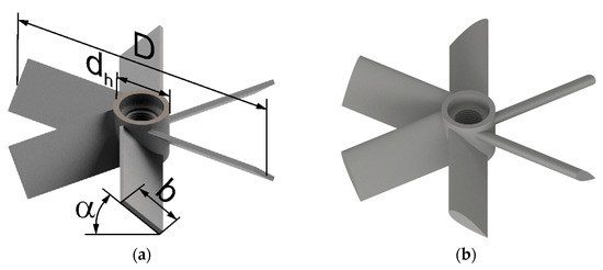
Figure 2.
PBT impellers with flat profile (a) and airfoil profile (b).
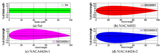
Figure 3.
Blade profiles: (a) rectangular (flat), (b) symmetrical NACA0021, (c,d) asymmetrical NACA4424.
As shown in Figure 3, the asymmetrical profile NACA4424 can be positioned in two ways relative to the direction of movement, as shown in Figure 4, where the arrows show the direction of the blade movement. The forces acting on the blade set as in Figure 4b,c will be identical, but for the setting in Figure 4c (negative angle of attack), the drag coefficient values should be more accessible, at least for small angles of attack. Therefore, in subsequent parts of the paper, the flow of the impeller blade set as shown in Figure 4c is analyzed.
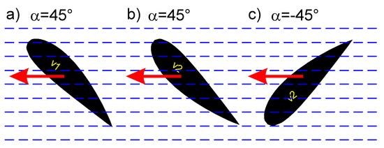
Figure 4.
Positioning of asymmetrical profile. (a) normal profile setting as in airplane wing (b) reverse positioning of the profile (upside down) (c) setting equivalent to setting (b).
Despite the fact that the profiles that were used were developed many years ago, they are still being studied [45]. The impellers shown in Figure 2 with the cross-sections of the blades as shown in Figure 3 were made using the 3D printing technique.
2.1. Measurements of the Liquid Velocity in the Mixer
Measurements of velocity distributions in the vertical r–z plane were carried out in a transparent vessel with a diameter T = 292 mm with a flat bottom and filled with distilled water to a height H = 300 mm (H ≅ T). Inside the tank, there were four standard baffles with a width of B = 0.1⋅T placed at equal intervals. A PBT45-6 turbine-blade impeller with a diameter of D = 100 mm suspended at a height of Z = 100 mm above the bottom of the tank was tested. As flow markers hollow glass spheres with an average diameter of 10 µm were used. To reduce the possibility of optical distortions, the cylindrical vessel was placed in an additional rectangular glass container also filled with water. Based on the analysis of the results of preliminary measurements, the rotational frequency of the stirrer was limited to two limit values: N = 90 min−1 (Frm = 0.023, Rem = 15,000) and N = 240 min−1 (Frm = 0.163, Rem = 40,000). The direction of rotation of the impeller was selected so that the liquid flowing through the impeller zone was directed down the mixer as is appropriate when mixing suspension under industrial conditions.
The measurements were performed using the LaVision PIV measurement system with a two-pulse laser with a maximum power of 135 mW and an ImagePro camera with a resolution of 2048 px × 2048 px with a Nikkor 1.8/50 lens. The lens aperture was closed to the value ensuring the maximum resolution (i.e., the aperture value was 5.6 [46]).
In the measurements, the plane of the light knife was placed about 2° before the baffle. The diagram of the light knife position is shown in Figure 5. The measurement field was approximately 300 mm × 300 mm. The frequency of the laser double flashes (pulses) was 2.7 Hz. Thus, the images were recorded for different positions of the blades in relation to the plane of the light knife. For the double laser flash, the intervals were Dt = 4200 µs for N = 90 min−1 and Δτ = 1900 µs for N = 240 min−1 and were determined for the velocity of 0.65·Utip and the shift of the tracer particles 10 px. The DaVis 7.2 program uses sub-pixel interpolation, and under these conditions the particle displacement is estimated up to 0.1 pixels. This means that the expected velocity accuracy is σu = 0.1/(M·Δτ), where M is the magnification factor (M = 6.83 px/mm). The calculated estimated accuracy of the instantaneous velocity measurement is 0.0032 m/s and 0.0077 m/s respectively. For each rotational frequency and blade cross-section, 100 image pairs were taken to average the results [47]. The proprietary program DaVis 7.2 was used for data processing. Two-pass data processing was used with the final size of the analyzed field 32 px × 32 px (i.e., approximately 4.7 mm × 4.7 mm) without overlapping. To make comparisons easier, measured liquid velocities were divided by the tangential velocity of the blade tip to obtain a dimensionless value.
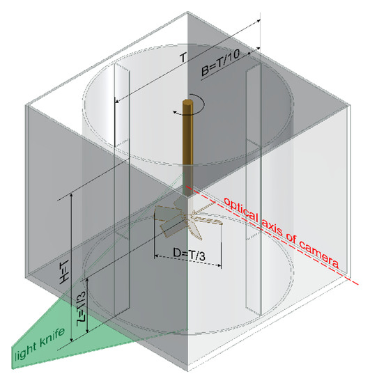
Figure 5.
Position of the light knife during the measurement of the components of radial and axial velocity.
2.2. Measurements of Mixing Power
The measurements of the mixing power were carried out in a flat-bottomed tank with a diameter of T = 400 mm, equipped with four standard baffles (B = 0.1·T). The tank was filled with water (t = 20°) to the height of H = T = 400 mm. For the tests impellers with a diameter of D = 133 mm (T/D = 3) were used. This system was geometrically similar to the system with a diameter of D = 292 mm shown in Figure 5, in which measurements of velocity distributions were made.
Torque measurements were made with the IKA EURO-ST P CV meter. Measurement data were recorded using the Labworldsoft 4.6 program with the sampling time Δt = 2 s. The values of the torque M were recorded for the set rotational frequency of the impeller N. The rotational frequency was changed within the range from N = 50 min−1 to N = 400 min−1, which corresponds to the values of Reynolds number for the mixing process from 14,750 to 118,000.
The measured values of the rotational frequency N and the torque M were used to calculate the mixing power number according to the relationship
3. Results and Discussion
3.1. Power Consumption
The measurements were carried out for the turbulent mixing range (Rem > 10000 [3,4]) in which the power number Po had a constant value. The obtained values of the power number depending on the blade profile are presented in Figure 6. The values Po were obtained with an error of ±4.2%. The figure also shows the percentage reduction in the mixing power of impellers with a profiled cross-section in relation to standard impeller PBT45-6.
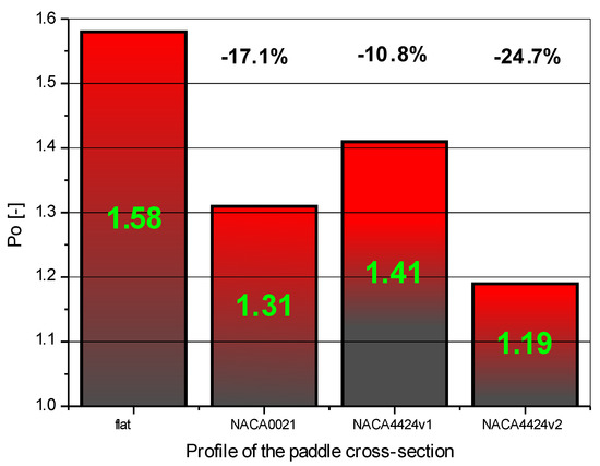
Figure 6.
Mixing power numbers of the tested impeller designs.
The mixing power number Po for the standard PBT impeller obtained in the tests was similar to the values given in the literature and presented in Table 1.

Table 1.
Mixing power number.
In all cases, impellers with aerodynamic profile blades have lower power consumption than the standard impeller. This is a result of the lower resistance during the impeller rotation, according to Equation (8). This is especially evident for the setting variants of NACA4424 profile. The profile is non-symmetrical, and shows different values of the drag coefficients for the angles of attack α with opposite signs. In Figure 7, positive angles α correspond to variant 1, and negative angles to variant 2 (Figure 4).
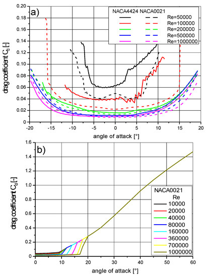
Figure 7.
Dependence of drag coefficient on the angle of attack [53,54,55]. (a) the drag coefficient of the airfoil NACA0021 for small angles of attack (b) the drag coefficient of the airfoil NACA0021 for high angles of attack.
Impellers with airfoil blades have a lower power consumption than a standard impeller. This is most likely due to the lower resistance to the stirrer’s rotation, as described in Equation (8). Since the drag coefficient Cd depends on the angle of attack α, it is an analogous relationship, although not to such an extent, can be observed when comparing the mixing power for PBT mixers with a rectangular cross-section with different blade inclination angles [12,35,48,52]. Most of the available data [53,54] determining the relationship Cd = f(α, Re) concern small angles of attack (Figure 7a). On the basis of these data, the relationship presented in Figure 6 can be partially explained. However, as shown by some data presented in the literature [55], for larger angles of attack (>20°), there is an increase in the value of the drag coefficient and the disappearance of the dependence on the Reynolds number (Figure 7b). Meanwhile, the phenomenon of an abrupt increase in the drag coefficient is not observed in the case of a flat plate [56].
No dependence Cd = f(Re) means that the value of the drag coefficient will not change depending on the distance from the axis of rotation of the impeller This facilitates the analysis of the dependence of the mixing power depending on the aerodynamic profile used, provided that the value of the drag coefficient Cd is known. Due to the lack of information on the values of the drag coefficient for the NACA4424 profile for angles of attack greater than 20°, an attempt was made to determine them based on numerical CFD simulations. This is a rapidly developing branch of computer science, although the results obtained in simulations are still verified experimentally [56,57,58]. The calculations were carried out in the ANSYS CFX program for the channel (dimensions: length Lch = 300 mm, height Hch = 125 mm, width Bch = 10 mm), in which water flowed at the speed Uch = 0.15 m/s. The used profile had a chord length of 100 mm, which gives a Reynolds number value for the flow of around Ref = 15,000. The dimensions of the channel correspond to the channel of the stand for testing the spray detachment angles. The turbulence model was used in the calculations: k—ε. The results obtained for both variants of the NACA4424 profile setting for the angle of attack α = 45° are shown in Figure 8 [59].
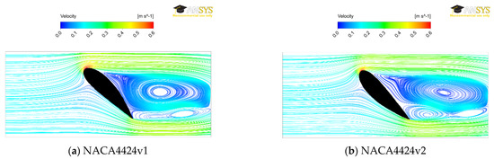
Figure 8.
Stream lines during the flow around the blade in the channel. (a) for normal setting, (b) for reverse setting.
Both the experimental results and the simulation show differences in the flow around the profiles by the fluid, especially behind the profile. In variant 2 (right figure), the stream tears off faster. The values of the force acting on the profile in the direction of flow (drag forces) calculated by the ANSYS CFX program are summarized in Table 2.
Table 2.
Calculated drag forces for narrow channel.
For a plate and a symmetrical profile, the Fx values for negative and positive angles are equal. In the case of a non-symmetrical profile, the drag force depends significantly on the profile setting. In the case of the flow around the aerodynamic profiles, significantly lower drag forces were obtained.
As the projection areas on the plane perpendicular to the flow direction were the same, it can be concluded that Cd ∝ Fx. However, full compliance with the mixing power data presented in Figure 6 has not been achieved. For the NACA4424 profile and the angle of attack of +45°, the drag force is lower than for the NACA0021 profile, although the comparison of the power shows that it should be the opposite. As there is a strong influence of the walls on the flow in the tested tunnel, calculations were made for a larger tunnel (dimensions: length Lch = 1500 mm, height Hch = 1370 mm, width Bch = 750 mm). The length of the chord was 100 mm, and the length of the plane was 200 mm. The results are shown in Table 3.
Table 3.
Calculated drag coefficients.
When the tunnel walls do not affect the flow of the profile, better compliance with the results of mixing power measurements was obtained, but the values of the proportionality coefficients are different than those obtained in the measurements of mixing power. The reason for the discrepancy may be an influence of the influence of centrifugal force not taken into account. It may also result from calculation errors caused by many factors (adopted turbulence model, mesh density, etc.). This is evidenced by the inflated results obtained in these conditions for the sphere. Therefore, the CFD method gives encouraging results to confirm the validity of Relationship (8), but requires further detailed research. These studies should also explain the influence of induced drag on power consumption.
3.2. Flow Pattern
The measurements of axial and radial velocity distributions in a mixing tank with four standard baffles for the PBT45-6 impeller with a flat blade cross-section and for profiled cross-section blades were carried out using the PIV method. The obtained results are presented in Figure 9 in the form of dimensionless contour and vector maps U* = U/Utip = U/(π·D·N) = f(H*, R*) for the rotational frequency N = 240 min−1 (Re = 40,000). The presented graphs show the position of the circulation core, i.e., the point where radial and axial velocities marked as two intersecting red lines are equal to zero.
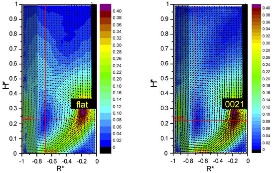
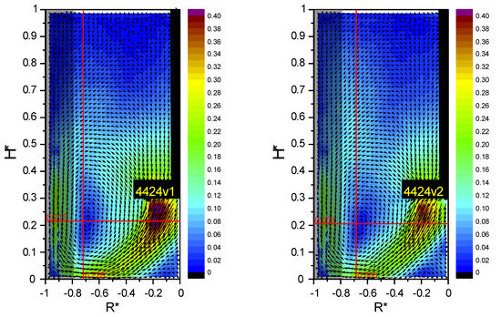
Figure 9.
Dimensionless velocity maps for N = 240 min−1 in the axial–radial plane.
Despite significant differences in the design of the impellers, for all tested cases, very similar liquid flow maps were obtained. The liquid flowed out from the impeller space downwards, but about 25 mm (0.09·H) from the lower edges of the blades, the liquid stream was already flowing at an angle of about 45° to the tank axis. There was always a conical space under the impeller with a slight but rising movement of the liquid. When mixing suspensions, this is called “dead space”. In this space, a swirling cone of grains that are not dispersed in the liquid can be formed. After reaching the bottom, the liquid stream changes the flow direction and flows radially towards the wall at a velocity of approximately 0.2·Utip, which allows the suspension grains to be lifted. At the contact area of the bottom and the cylindrical wall, there is another “dead zone” in which solid grains can accumulate. The obtained velocity map explains why a flat-bottomed tank is not an optimal structure for mixing suspensions [60,61]. At the wall, the liquid changes its direction again and flows upwards, reducing its speed and at the height of the impeller moves towards the tank axis and thus the circulation loop is closed. Above half of the tank height, the movement of the liquid is relatively slow, and the resultant velocity in this area is below 0.1·Utip.
For the NACA4424v2 profile only did the flow pattern differ from the others with respect to numerical velocity values, with the area of the highest velocities under the impeller being smaller than in other cases. Furthermore, in this case, the width of the liquid stream directed to the tank bottom was the smallest. As a result, the conical space under the impeller, in which the liquid flows at a very low speed upward, was the greatest. As mentioned above, this is the flow “dead zone”.
The knowledge of the axial velocity distribution in the stream of liquid flowing at the wall of the mixing tank upwards is important, as it makes it possible to determine the size of solid particles that can be lifted from the bottom of the tank based on the particle settling velocity [62].
3.3. Pumping Capacity and Secondary Circulation Rate
On the basis of the velocities determined by the PIV measuring system, the axial velocity profiles were determined directly under the impeller, i.e., approximately 1 mm below the lower edge of the impeller blades. The results obtained for N = 90 and 240 min−1 are shown in Figure 10.
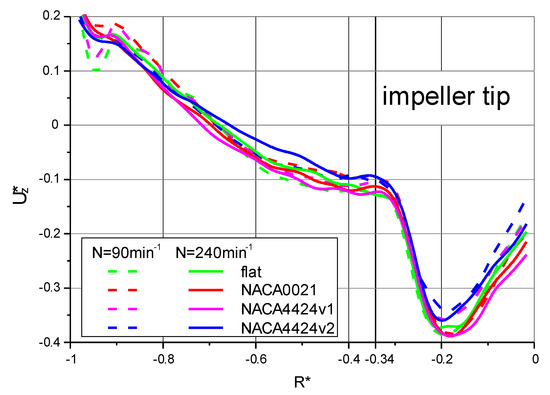
Figure 10.
Axial dimensionless velocity profiles 1 mm below the impeller.
The shapes of individual curves obtained in Figure 10 for the three impellers with NACA profiled blades and for the standard PBT45-6 impeller are similar to each other and coincide to a great extent with the results of other authors obtained for the standard PBT impeller [22,63,64]. It should be noted that the maximum values of axial velocities in the stream of liquid pumped from the impeller zone downwards occur in the half of the radius of the impeller they are included within narrow limits of (0.35 ÷ 0.39)·Utip. The remaining stream of induced circulation also flowing downwards has a much lower velocity, on average about 0.08·Utip, as this stream does not pass through the area of the impeller. The impeller with a rectangular cross-section of the blades, despite higher power consumption (Figure 5), does not show higher axial velocities compared to the impellers with a profiled section, except for the NACA4424v2 impeller. The other two NACA impellers showed even slightly higher axial velocities than the standard PBT45-6 impeller, despite lower mixing powers. This is important because liquid with higher axial velocity has a greater chance of picking up solid particles resting there and suspending them in the liquid core.
The same circulation stream of liquid flowing upwards near the wall of the mixing tank already has a velocity that is half that of the downward flow. This is due to the fact that it flows through a larger cross-section of the mixing tank than before. The same diagram shows that the analogical courses of the curves were obtained also for almost three times lower rotational frequencies of the impellers N = 90 min−1.
On the basis of the velocity profiles obtained in Figure 10, pumping capacity Vpump and flow-rate number Flpump were calculated using the numerical integration methods. The results are shown in Table 4.
Table 4.
Pumping capacity.
The values of the pumping number Flpump for the standard PBT45-6 impeller presented in Table 2 for are slightly higher than the Flpump = 0.58 value given by Medek and Fořt [65], obtained by the flow follower method, but lower than the Flpump = 0.73 obtained by the LDA method by Nienow [13]. A very similar value of Flpump = 0.68 is given by Aubin [11], and this value was obtained using the PIV method. Many authors present the obtained results in the form of correlation equations from which the Flpump value can be calculated. Doran [66] quotes Equations (10) and (11) which make Flpump values are dependent only on the power number Po
from which, after adopting the value of Po = 1.58, we obtain Flpump = 0.99 and Flpump = 0.88, respectively. This probably results from the fact that in the correlation dependencies errors related to the determination of the power number Po and errors related to the determination of a specific correlation equation accumulate. Hence their lower accuracy. The value 0.79 is given in Paul’s monograph [14]. On the other hand, in the monograph by Uhl and Gray [1], there is a relationship
However, the numerical values of Flpump obtained from Equations (10)–(12) were most often greater than the values of the Flpump pumping numbers for the axial flow impellers presented in Table 4. Hence their lower accuracy. Therefore, in the further part of the work, the Flpump values obtained in the own research were used.
To calculate the mixing time 𝜏m, it is necessary to know the circulation time 𝜏c determined by Equation (2). This, in turn, requires the knowledge of the value of the radial-axial circulation, i.e., secondary circulation Vs. This is the volumetric flow rate of liquid in the r–z plane in the entire mixing tank. This value is usually given in the form of the dimensionless secondary circulation number Fls
To determine the amount of the secondary circulation Vs, the axial velocity profiles were determined in the mixing tank at the height of the circulation core (Figure 9). The obtained results are shown in Figure 11. Due to the fact that the planes passing through the individual circulation cores are located near the lower edge of the rotating blades of the impeller, the obtained axial velocity distributions in Figure 11 are very similar to the distributions presented in Figure 10. By numerical integration of the distribution presented in Figure 11, it was possible to obtain the value of the entire stream Vs circulating in the plane r–z.
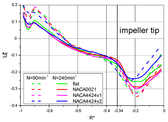
Figure 11.
Profiles of axial dimensionless velocities at the height of the circulation core.
In the next step, the dimensionless secondary circulation Fls and the circulation time 𝜏c from Equation (2) were calculated. The results are included in Table 5, which additionally presents the Vs/Vpump ratio. It should be emphasized that the entire secondary circulation in of the mixer Vs is the sum of the pumping capacity Vpump and the induced circulation Vi due to existing viscosity of the real fluids and the simultaneous stream momentum transfer Vpump.
Table 5.
Circulation capacity.
Usually, the induced stream Vi is 5–10% lower than the stream Vpump pumped by the impeller and therefore the entire secondary circulation Vs is usually twice as high as the Vpump value. The data included in Table 5 confirm this observation [3,4,65].
3.4. Efficiency
Final results concerning the research on the efficiency of any process very often depend on the adopted optimization criterion. Two optimization criteria were examined in this study. The first was the criterion proposed by Nienov [13]; in the second case, a method based on the mixing energies UE determined in this study was proposed.
In the first case, from Equation (4) [13], the mixing efficiency Ep was determined for the obtained Flpump numbers, included in Table 4 for N = 90 min−1 and N = 240 min−1. The obtained results are summarized in Table 6.
Table 6.
Efficiency of impellers.
The analysis in Table 6 shows that for the lower rotational frequency of the impeller, N = 90 min−1, the highest efficiency, i.e., the highest Ep values, was obtained for the impeller with a flat cross-section (gray cells), and the impeller with a symmetrical NACA0021 profile was in the second place (fewer gray cells). For the higher of the tested rotational frequencies, N = 240 min−1, the most effective design was the impeller with the NACA4424v1 profile set with the flatter side in the direction of movement; but again, the impeller with the symmetrical profile NACA0021 was in second place. The observed differences are currently difficult to explain. They may, for example, result from the difference in the values of drag coefficients Cd in Figure 7 for individual profiles, and the mixing power in turbulent flow depends on the Cd value.
In the second case, the mixing efficiency of the tested impeller was calculated on the basis of the UE mixing energy determined by Equation (1), which after taking into account Equation (3) takes the following form:
The mixing power P of individual PBT45-6 impeller was calculated on the basis of the power number values Po = const. shown in Figure 6, while the circulation time τc was taken from the experimental data shown in Table 3. The results of the calculations of mixing energy UE for the tested impellers for two rotational frequencies of the impellers N = 90 min−1 and for N = 240 min−1 are presented in Table 7. As with the application of the Nienov criterion [13], the obtained results depend on the rotational frequency. For N = 90 min−1, the lowest values of mixing energy UE were obtained for NACA4424v2 system (Figure 6), and for N = 240 min−1, the most effective impeller was NACA0021. Meanwhile, regardless of the rotational frequency, the impeller with flat blades was the worst.
Table 7.
Mixing efficiency.
For all impellers, the obtained values of the mixing energy UE were about seven times higher for the higher rotational frequencies N = 240 min−1 than for the frequency N = 90 min−1. This is undoubtedly the cost that must be incurred to obtain almost three times shorter mixing time 𝜏m (Table 7).
A certain disadvantage in the practical application of the dimension criterion UE is its dependence on the rotational frequency N of the impeller. This can be avoided by transforming Equation (14). Introducing Equations (2), (3) and (13) into it and expressing the power P on the basis of the definitional power number equation Po (Equation (9)), we get Expression (15), which can be treated as a definition of the dimensionless mixing energy for turbulent motion.
It is worth noting that the expression in the denominator of Equation (15) is proportional to the kinetic energy of the liquid in the mixing tank. The lower the value of , the more effective the conversion of the mechanical energy supplied to the mixing tank into the kinetic energy of the mixed liquid (N2 D2 ρ).
Table 7 summarizes the values for individual impellers. Due to the fact that a dimensionless optimization criterion was used, the values for individual impellers changed slightly when the rotational frequency N was changed. This is a significant advantage of the dimensionless criterion in relation to the dimension criterion UE.
It should be noted that both adopted optimization criteria based on the mixing energy are insensitive to changes in the assumed factor, which is equal to 4 in Equation (3). Assuming a different value of this coefficient will only cause a parallel shift of the obtained results, while the final optimization result will be the same.
4. Conclusions
In turbulent motion, PBT impellers with an airfoil paddle cross-section displayed a reduction of 11% to 25% of mixing power compared to PBT45-6 flat paddle impellers. However, both types of impellers showed a similar secondary circulation flow in the stirred vessel.
Regardless of the applied optimization criterion, the NACA0021 impeller with symmetrical cross-section has always been one of the top two most effective impellers. Its mixing energy at higher rotational frequencies was 20% lower than for the standard PBT45-6 impeller.
Dimensionless optimization criterion is more general than the dimensional criterion because its value does not depend on the rotational frequency of the impeller.
Due to the rapid development of 3D printers, impellers with profiled blades can be used more often, even in industrial conditions, in the future.
Author Contributions
Conceptualization, J.S. and C.K.; methodology, J.S. and F.R.; software, J.S.; validation, F.R. and R.M.; formal analysis, T.J and F.R.; investigation, R.M., C.K. and J.S.; resources, T.J. and F.R.; data curation, J.S.; writing—original draft preparation, C.K. and J.S.; writing—review and editing, J.S. and C.K.; visualization, J.S.; supervision, F.R and T.J.; project administration, T.J. and J.S.; funding acquisition, T.J. and F.R. All authors have read and agreed to the published version of the manuscript.
Funding
This research was funded by the Ministry of Education, Youth and Sports of the Czech Republic: OP RDE CZ.02.1.01/0.0/0.0/16_019/0000753.
Institutional Review Board Statement
Not applicable.
Informed Consent Statement
Not applicable.
Data Availability Statement
Not applicable.
Acknowledgments
The work was created as part of the statutory activity of the Department of Chemical Engineering of Lodz University of Technology and the grant OP RDE CZ.02.1.01/0.0/0.0/16_019/ 0000753 financed by the Ministry of Education, Youth and Sports of the Czech Republic.
Conflicts of Interest
The authors declare no conflict of interest.
List of Symbols
| b | blade width, m |
| B | baffle width, m |
| C | chord length, m |
| Cd | drag coefficient, |
| Cl | lift coefficient, |
| dh | hub diameter, m |
| D | impeller diameter, m |
| E | mixing energy, J |
| Ep | dimensionless efficiency criterion, |
| F | force (in general), N |
| g | acceleration of gravity, m/s2 |
| N | rotation frequency, s−1 |
| H | water height, m |
| H* | dimensionless height (here H* = H/300 mm), |
| M | magnification factor, pixel/mm |
| P | mixing power, W |
| R | radius, m |
| R* | dimensionless radius (here R* = R/146 mm), - |
| T | tank diameter, m |
| U | velocity (in general), m/s |
| U* | dimensionless velocity, - |
| UE | mixing efficiency, J/m3 |
| U*E | dimensionless mixing efficiency, - |
| Utip | velocity of the end of impeller blade, m/s |
| Uz | axial velocity, m/s |
| V | volume of the mixed liquid, m3 |
| Vpump | pumping capacity, m3/s |
| Vs | secondary circulation in the stirred vessel, m3/s |
| Z | distance of the impeller from the bottom, m |
Greek Letters
| α | blade inclination, angle of attack, ° |
| η | dynamic viscosity, Pa·s |
| ρ | density, kg/m3 |
| τc | circulation time, s |
| τm | mixing (homogenization) time, s |
| Δτ | interval for double laser pulses, s |
Dimensionless Numbers
| flow number for secondary circulation | |
| flow number for impeller pumping | |
| Froude number for mixing process | |
| power number for mixing process | |
| Reynolds number for mixing process | |
| Reynolds number for flow around airfoil |
References
- Fořt, I. Flow and turbulence in vessels with axial impellers. In Mixing: Theory and Practice; Uhl, V.W., Gray, J.B., Eds.; Academic Press, Inc.: London, UK, 1986; Volume 3, pp. 133–197. [Google Scholar]
- Stelmach, J.; Kuncewicz, C.Z. Effect of propeller impeller blade profile on hydrodynamics and power consumption. Przem. Chem. 2017, 96/11, 2348–2352. (In Polish) [Google Scholar]
- Stręk, F. Mieszanie I Mieszalniki; WNT: Warszawa, Poland, 1981; pp. 135–148. (In Polish) [Google Scholar]
- Nagata, S. Mixing. Principles and Applications; John Wiley & Sons: New York, NY, USA, 1975; pp. 126–178. [Google Scholar]
- Guerin, P.; Carreau, P.J.; Patterson, W.I.; Paris, J. Characterization of helical impellers by circulation times. Can. J. Chem. Eng. 1984, 62, 301–309. [Google Scholar] [CrossRef]
- Delaplace, G.; Leuliet, J.C. Circulation and mixing times for helical ribbon impellers. Review and Experiments. Exp. Fluids 2000, 28, 170–182. [Google Scholar] [CrossRef]
- Trambouze, P.; Euzen, J.P. Chemical Reactors: From Design to Operations; Edition TECHIP: Paris, France, 2004. [Google Scholar]
- Rieger, F.; Novák, V.; Jirout, T. Hydromechanické Procesy II; CTU Publishing House: Praha, Czech, 2007. [Google Scholar]
- Fořt, I.; Sedláková, V. Studies on mixing. XX. Pumping effect of high-speed rotary mixers. Collect. Czecoslov. Chem. Commun. 1968, 33, 836–849. [Google Scholar] [CrossRef]
- Kawase, Y.; Moo-Young, M. Mathematical models for design of bioreactors: Application of Kolmogoroff’s theory of isotropic turbulence. Chem. Eng. J. 1990, 43, 19–41. [Google Scholar] [CrossRef]
- Aubin, J.; Mavros, P.; Fletcher, D.E.; Bertrand, J.; Xuereb, C. Effect of axial agitator configuration (up-pumping, down-pumping, reverse rotation) on flow patterns generated in stirred vessels. Trans. IChemE. 2001, 79, 845–856. [Google Scholar] [CrossRef]
- Kumeresan, T.; Joshi, J.B. Effect of impeller design on the flow pattern and mixing in stirred tanks. Chem. Eng. J. 2006, 115, 173–193. [Google Scholar] [CrossRef]
- Nienow, A.W. On impeller circulation and mixing effectiveness in the turbulent flow regime. Chem. Eng. Sci. 1997, 52, 2557–2565. [Google Scholar] [CrossRef]
- Hemrajani, R.R.; Tatterson, G.B. Mechanically stirred vessels. In Handbook of industrial Mixing: Science and Practice; Paul, E.L., Atiemo-Obeng, V.A., Kresta, S.M., Eds.; John Wiley & Sons. Inc.: Hoboken, NJ, USA, 2004; pp. 345–390. [Google Scholar]
- Kurasiński, T.; Kuncewicz, C.Z.; Stelmach, J. Method of convective velocity determination from dissipative range of energy spectrum. Chem. Proc. Eng. 2011, 33, 19–29. [Google Scholar] [CrossRef]
- Giacomelli, J.J.; Van der Akker, H.E.A. Time scales and turbulent spectra above the base of stirred vessels from large eddy simulations. Flow Turbul. Combust. 2020, 105, 31–62. [Google Scholar] [CrossRef]
- Talaga, J.; Duda, A. Determination of macro- and microscale turbulence of liquid in a mixing vessel on the basis of autocorrelation function. Inż. Ap. Chem. 2004, 42, 152–154. (In Polish) [Google Scholar]
- Kresta, S. Turbulence in stirred tanks: Anisotropic, approximate and applied. Can. J. Chem. Eng. 1998, 76, 563–576. [Google Scholar] [CrossRef]
- Ng, K.; Yianneskis, M. Observations on the distribution of energy dissipation in stirred vessels. Trans. IchemE. 2000, 78, 334–341. [Google Scholar] [CrossRef]
- Sheng, J.; Meng, H.; Fox, R.O. A large eddy PIV method for turbulence dissipation rate estimation. Chem. Eng. Sci. 2000, 55, 4423–4434. [Google Scholar] [CrossRef]
- Baldi, S.; Yianneskis, M. On the direct measurement of turbulence energy dissipation in stirred vessels with PIV. Ind. Eng. Chem. Res. 2003, 42, 7006–7016. [Google Scholar] [CrossRef]
- Gabriele, A.; Nienow, A.W.; Simmons, M.J.H. Use of angle resolved PIV to estimate local specific energy dissipation rate for up- and down-pumping pitched blade agitators in a stirred tank. Chem. Eng. Sci. 2009, 64, 126–143. [Google Scholar] [CrossRef]
- Delafosse, A.; Collignon, M.-L.; Crine, M.; Toye, D. Estimation of the turbulent kinetic energy dissipation rate from 2D-PIV measurements in a vessel stirred by an axial Mixel TTP impeller. Chem. Eng. Sci. 2011, 66, 1728–1737. [Google Scholar] [CrossRef]
- Xu, D.; Chen, J. Accurate estimate of turbulent dissipation rate using PIV data. Exp. Therm. Fluid Sci. 2013, 44, 662–672. [Google Scholar] [CrossRef]
- Linek, V.; Kordač, M.; Fujasová, M.; Moucha, T. Gas-liquid mass transfer coefficient in stirred tanks interpreter through models of idealized eddy structure of turbulence in the bubbly vicinity. Chem. Eng. Proc. 2004, 43, 1511–1517. [Google Scholar] [CrossRef]
- Alves, S.S.; Vasconcelos, J.M.T.; Orvalho, S.P. Mass transfer to clean bubbles at low turbulent energy dissipation. Chem. Eng. Sci. 2006, 61, 1334–1337. [Google Scholar] [CrossRef]
- Garcia-Ochoa, F.; Gomez, E. Theoretical prediction of gas-liquid mass transfer coefficient, specific area and hold-up in sparged stirred tanks. Chem. Eng. Sci. 2004, 59, 2489–2501. [Google Scholar] [CrossRef]
- Zhou, G.; Kresta, S.M. Correlation of mean drop size and minimum drop size with the turbulence energy dissipation and the flow in an agitated tank. Chem. Eng. Sci. 1998, 53, 2063–2079. [Google Scholar] [CrossRef]
- Alopaeus, V.; Koskinen, J.; Keskinen, K.I. Simulation of the population balance for liquid-liquid systems in a nonideal stirred tank. Part 1 Description and qualitive validation of the model. Chem. Eng. Sci. 1999, 54, 5887–5899. [Google Scholar] [CrossRef]
- Podgórska, W. Theoretical and experimental investigation of the influence of dispersed phase viscosity on drop coalescence. In Proceedings of the 12th European Conference on Mixing, Bologna, Italy, 27–30 June 2006; pp. 303–310. [Google Scholar]
- Podgórska, W.; Bąk, A. Modeling of drop coalescence in stirred liquid-liquid dispersion containing surfactant. In Proceedings of the 14th European Conference on Mixing, Warsaw, Poland, 10–13 September 2012; pp. 383–394. [Google Scholar]
- Schäfer, M.; Yianneskis, M.; Wächter, P.; Durst, F. Trailing vortices around a 45° pitched-blade impeller. Fluid Mech. Transport. Phenom. 1998, 44, 1233–1246. [Google Scholar] [CrossRef]
- Amira, B.B.; Driss, Z.; Karray, S.; Abid, M.S. PIV Study of the Down-Pitched Blade Turbine Hydrodynamic Structure. In Design and Modeling of Mechanical Systems, Proceedings of the Fifth International Conference on Design and Modeling of Mechanical Systems, CMSM’2013, Djerba, Tunisia, 25–27 March 2013, 2013 ed.; Haddar, M., Romdhane, L., Louati, J., Ben Amara, A., Eds.; Springer: Berlin/Heidelberg, Germany, 2013; pp. 237–244. [Google Scholar]
- Amira, B.B.; Driss, Z.; Abid, M.S. Experimental study of the 60° PBT6 pitching blade effect with PIV application. In Multiphysics Modelling and Simulation for Systems Design and Monitoring, Applied Condition Monitoring; Haddar, M., Abbes, M.S., Choley, J.-Y., Boukharouba, T., Elnady, T., Kanaev, A., Amar, M.B., Chaari, F., Eds.; Springer: Singapore, 2015; pp. 91–100. [Google Scholar]
- Ameur, H. Energy efficiency of different impellers in stirred tank reactors. Energy 2015, 93, 1980–1988. [Google Scholar] [CrossRef]
- Axial Flow Impeller Shapes: Part 1. Available online: https://www.academia.edu/9425356/Axial_flow_impeller_shapes_part_1 (accessed on 30 December 2021).
- Axial flow Impeller Shapes: Part 2. Available online: https://www.academia.edu/9425356/Axial_flow_impeller_shapes_part_2 (accessed on 30 December 2021).
- Stelmach, J.; Kuncewicz, C.Z.; Szufa, S.; Jirout, T.; Rieger, F. The influence of hydrodynamic changes in a system with a pitched blade turbine on mixing power. Processes 2021, 9, 68. [Google Scholar] [CrossRef]
- Hamill, G.A.; Kee, C. Predicting axial velocity profiles within a diffusing marine propeller jet. Ocean Eng. 2016, 124, 104–112. [Google Scholar] [CrossRef]
- Singh, P.; Nestmann, F. Exit blade geometry and part-load performance of small axial flow propeller turbines: An experimental investigation. Exp. Therm. Fluid Sci. 2010, 34, 798–811. [Google Scholar] [CrossRef]
- Ghosh, P.; Dewangan, A.K.; Mitra, P.; Rout, A.K. Experimental Study of Aero Foil with Wind Tunnel Setup. 2014. Available online: https://www.researchgate.net/publication/259739000 (accessed on 30 December 2021).
- Sreedevi, K.N.V.; Krishna, M.V.S. Effect of Angle of Attack on Aerodynamic Forces of Symmetrical and Unsymmetrical Airfoil Using Windtunnel. 2020. Available online: https://www.researchgate.net/publication/345477933 (accessed on 30 December 2021).
- Llorente, E.; Gorostidi, A.; Jacobs, M.; Timmer, W.A.; Munduate, X.; Pires, O. Wind Tunnel Tests of Wind Turbine Airfoils at High Reynolds Numbers. 2014. Available online: https://www.researchgate.net/publication/263128323 (accessed on 30 December 2021).
- Ortiz, X.; Rival, D.; Wood, D. Forces and moments on flat plates of small aspect ratio with application to pv wind loads and small wind turbine blades. Energies 2015, 8, 2438–2453. [Google Scholar] [CrossRef]
- Surekha, D.R.S.; Khandelwal, A.; Rajasekar, R. Investigation of flow field in deep dynamic stall over an oscillating NACA0012 airfoil. J. Appl. Fluid Mech. 2019, 12, 857–863. [Google Scholar]
- Test Obiektywu. Available online: www.optyczne.pl/66.4-Test_obiektywu-Nikon_Nikkor_AF_50_mm_f_1.8D_Rozdzielczo%C5%9B%C4%87_obrazu.html (accessed on 3 November 2021).
- Heim, A.; Stelmach, J. The comparison of velocities at the self-aspirating disk impeller level. Przem. Chem. 2011, 90, 1642–1646. (In Polish) [Google Scholar]
- Major-Godlewska, M.; Karcz, J. Power consumption for an agitated vessel equipped with pitched blade turbine and short baffles. Chem. Papers 2018, 72, 1081–1088. [Google Scholar] [CrossRef] [PubMed]
- Medek, J.; Fořt, I. Pumping effect of impellers with float inclined blades. Collect. Czech. Chem. Commun. 1979, 44, 3077–3089. [Google Scholar] [CrossRef]
- Tsui, Y.-Y.; Chou, J.-R.; Hu, Y.-C. Blade angle effects on the flow in a tank agitate by the pitched-blade turbine. J. Fluids Eng. 2006, 128, 774–782. [Google Scholar] [CrossRef]
- Beshay, K.; Kratěna, J.; Fořt, I.; Brůha, O. Power input of high-speed rotary impellers. Acta Polytech. 2001, 41, 18–23. [Google Scholar] [CrossRef]
- Fořt, I.; Seichter, P.; Pešl, L. Axial thrust of axial flow impellers. Chem. Eng. Res. Des. 2013, 91, 789–794. [Google Scholar] [CrossRef]
- Airfoil Tools. Available online: Airfoiltools.com/airfoil/details?airfoil=naca0021-il (accessed on 3 November 2021).
- Airfoil Tools. Available online: Airfoiltools.com/airfoil/details?airfoil=naca4424-il (accessed on 3 November 2021).
- Aerodynamic Characteristics of Seven Symmetrical Airfoil Sections through 180-Degree Angle of Attack for Use in Aerodynamic Analysis of Vertical Axis Wind Turbines. Available online: https://www.osti.gov/servlets/purl/6548367 (accessed on 30 December 2021).
- Ortiz, X.; Hemmatti, A.; Rival, D.; Wood, D. Instantaneous forces and moments on inclined flat plates. In Proceedings of the 7th International Colloquium on Bluff Body Aerodynamics and Applications (BBAA7), Shanghai, China, 2–6 September 2012; Available online: https://citeseerx.ist.psu.edu/viewdoc/download?doi=10.1.1.1076.7687&rep=rep1&type=pdf (accessed on 3 November 2021).
- Khopkar, A.R.; Mavros, P.; Ranade, V.V.; Bertrand, J. Simulation of flow generated by an axial-flow impeller. Chem. Eng. Reas. Des. 2004, 82, 737–751. [Google Scholar] [CrossRef][Green Version]
- Hargreaves, D.M.; Kakimpa, B.; Owen, J.S. The computational fluid dynamics modelling of the autorotation of square, flat plates. J. Fluids Struct. 2014, 46, 111–133. [Google Scholar] [CrossRef]
- Bujak, K. Analysis of Liquid Hydrodynamics Near the Agitator Blades. Master’s Thesis, Lodz University of Technology, Lodz, Poland, 2021. (In Polish). [Google Scholar]
- Rieger, F.; Rzyski, E. Mixing of suspensions in tanks with an increased number of impellers. Chem. Proc. Eng. 2001, 22, 1213–1218. [Google Scholar]
- Rieger, F.; Jirout, T.; Rzyski, E. Mixing of suspensions. Selection of the mixer and tank. Inż. Ap. Chem. 2002, 41, 113–115. [Google Scholar]
- Atiemo-Obeng, V.A.; Penney, W.R.; Armenante, P. Solid-liquid mixing. In Handbook of Industrial Mixing: Science and Practice; Paul, E.L., Atiemo-Obeng, V.A., Kresta, S.M., Eds.; John Wiley & Sons. Inc.: Hoboken, NJ, USA, 2004; pp. 543–584. [Google Scholar]
- Fořt, I.; Jirout, T.; Sperling, R.; Jambere, S.; Rieger, F. Study of pumping capacity of pitched blade impellers. Acta Polytech. 2002, 42, 68–72. [Google Scholar] [CrossRef]
- Ge, C.-Y.; Wang, J.-J.; Gu, X.-P.; Feng, L.-F. CFD simulation and PIV measurement of the flow field generated by modified pitched blade turbine impellers. Chem. Eng. Res. Des. 2014, 92, 1027–1036. [Google Scholar] [CrossRef]
- Medek, J.; Fořt, I. Mixing in vessel with eccentrical mixer. In Proceedings of the 5th European Conference on Mixing, Würzburg, Germany, 10–12 June 1985; pp. 263–271. [Google Scholar]
- Doran, P.M. Design of mixing systems for plant cell suspension in stirred reactors. Biotechnol. Prog. 1999, 15, 319–335. [Google Scholar] [CrossRef] [PubMed]


Publisher’s Note: MDPI stays neutral with regard to jurisdictional claims in published maps and institutional affiliations. |
© 2022 by the authors. Licensee MDPI, Basel, Switzerland. This article is an open access article distributed under the terms and conditions of the Creative Commons Attribution (CC BY) license (https://creativecommons.org/licenses/by/4.0/).