Article

Numerical Investigation of Jet Control Using Two Pulsed Jets under Different Amplitudes

School of Energy and Power Engineering, Beihang University, Beijing 100191, China
*
Author to whom correspondence should be addressed.
Energies 2022, 15(2), 640; https://doi.org/10.3390/en15020640
Submission received: 6 December 2021 / Revised: 27 December 2021 / Accepted: 13 January 2022 / Published: 17 January 2022

Abstract

:
A turbulent jet with a Reynolds number of 71,000, controlled by a pair of pulsed jets operating 180° out of phase, is investigated by large-eddy simulation. The effect of the forcing amplitude on jet development and generated coherent structures is investigated through six cases: an unforced case and five cases at different amplitudes. With this forcing mode, the jet bifurcates in the far field that promotes the spread of the shear layer. It was found that the jet yields the largest bifurcation angle at medium amplitude, while the bifurcation is restrained at lower or higher amplitudes. As the amplitude increases, the streamwise vortex pair generated by the control jet is stronger and penetrates deeper into primary jet. This phenomenon reduces the inclination of vortex ring when mutual interaction between vortex ring and streamwise vortex pair occurs. Meanwhile, at higher amplitudes, the inclined vortex ring is stronger and unevenly distributed, prompting the jet bifurcation. In order to investigate the coupling effect of amplitude and frequency, different forcing frequencies were also simulated. The results demonstrated that the optimal frequency based on centerline velocity decay rate decreases with increasing amplitude; however, it eventually saturates around StD = 0.1.

1. Introduction

In recent years, flow control techniques for round jets have received wide attention. This is primarily due to their potential and capabilities for performance improvement in engineering applications, particularly in the aerospace field. For example, the control of the jet flow to enhance mixing with ambient air has the benefits in infrared signature reduction and noise suppression [1,2]. Compared to passive techniques, active flow control provides flexibility, since the control devices can be switched on or off on demand. When an active control system has been properly configured, it can provide comparable or even better performance and less flow loss compared to passive configurations [3].
Active control techniques usually introduce perturbation to the primary jet shear layer in order to modify the generation and evolution of large-scale structures [4]. Such structures, which include vortex rings and streamwise vortices, are dominant in jet development and primarily responsible for entrainment and mixing in different regions [5,6]. Current methods mainly include acoustic actuation, synthetic jets, plasma actuation and steady or pulsed control jets [7,8,9,10]. Control jets are convenient for injecting fluid into the flow and require only some additional piping. In the case of aircraft, air can be directly supplied from the aero-engine. Consequently, its setup is simpler than that of other methods which need extra perturbation generators. Furthermore, compared to steady control jets, pulsed jets can manipulate the primary jet more effectively [10]. The reason is that pulsed jets can not only penetrate the primary jet, but can also introduce periodic perturbation, which responds to the primary instabilities in the jet.
The forcing amplitude of the control jet, defined as the mass flow ratio of control jet to the primary jet ( M F R = m ˙ c o n t r o l   j e t s m ˙ p r i m a r y   j e t   ), is known as one of the most influential factors. Parekh et al. [11] observed that when two pulsed jets were used to actuate subsonic and supersonic jets, the jet mixing increased rapidly for injection mass flow ratios below 1%; however, at ratios approximately 2%, it quickly reached an asymptotic limit. New and Tay [12] used two steady control jets to investigate the effect of mass flow ratio on round jet structures. Their results revealed that the presence of secondary injection inhibited the large-scale vortex roll-ups and made the primary jet shear layer transit to turbulence earlier with increasing injection flow rate. Each injected secondary flow evolved into a counter-rotating vortex pair (CVP). As the mass flow ratio increased, the CVPs penetrated deeper into the primary jet until they eventually met. In their quantitative analysis, the centerline velocity decayed faster at higher injection rates, indicating improved mixing. Wickersham [13] used two pulsed control jets to actuate a turbulent jet in flapping mode, and systematically investigated the effect of frequency and amplitude on mixing enhancement. It was found that, initially, the mixing efficiency increased with forcing amplitudes; however, at higher amplitudes, the mixing efficiency was decreased. Moreover, it was found that the optimal frequency with respect to mixing efficiency decreased with increasing amplitude, which indicated a coupled relationship between these the two parameters. However, no clear explanation was proposed. The dependence of mixing efficiency on amplitude was also confirmed in the recent experimental works of Yang and Zhou and Perumal et al. [14,15]. In their works, two pulsed circular mini-jets excited a laminar jet in axisymmetric mode. They owed the different stages of amplitude effect to penetration depth. The structures produced by the min-jets were stronger and penetrated deeper into the primary jet with a higher mass flow ratio. Furthermore, these structures collided, impairing the strength and entrainment rate of the primary jet. When the amplitude was sufficiently high, the primary jet was initially fully turbulent; thus, the spreading rate could recover. The above studies all suggest that the forcing amplitude has a significant effect on coherent structures and mixing efficiency.
Bifurcating jets have gained much attention by researchers in jet control, since they greatly increase the spreading rate and accelerate the mixing with ambient flow compared to natural jets, suggesting possible applications in flow control. When a bifurcating jet is established with the right excitations, the jet is divided into two separate jets, each of which carries half the axial momentum and spreads in a manner similar to a single jet. The spreading rate increases dramatically in one plane (the bifurcating plane) and maintains or slightly reduces in the perpendicular plane (the bisecting plane) [16]. Lee and Reynolds [17] acquired a bifurcating jet by combining the axial and alternative helical actuation modes. They found that the ratio of the two excitation frequencies rf = fa/fh had an important effect on jet structures. More specifically, the bifurcating jet was acquired when rf = 2. Danaila and Boersma [18] conducted direct numerical simulation to investigate a low Reynolds number jet controlled by different forcing methods. The results showed that a solo flapping excitation with high amplitude could also make the jet bifurcate and the coherent structures in this jet were similar to those in a bifurcating jet acquired through combined excitations. Da Silva et al. [19] investigated the flapping mode excitation at preferred mode and the subharmonic frequencies. Both forcing methods succeeded in causing the jet bifurcation at low Reynolds numbers. Forcing at subharmonic frequency achieved better bifurcation and worked at higher Reynolds numbers. When the Reynolds number was beyond a certain value, the small-scale turbulence would cause the destruction of larger vortices so that the forcing method would lose its bifurcation effect.
In our previous study, it was found that the frequency of pulsed jets with flapping mode has a significant effect on large-scale structures and jet bifurcation [20]. Therefore, it is reasonable and attractive to research the effect of pulsed jet amplitude on coherent structures and jet bifurcation, which has not been extensively investigated. In the present work, several mass flow ratios (MFR = 0.67%, 0.83%, 1%, 1.2%, 1.5%, achieved by adjusting control jets velocity) at the same frequency (StD = 0.1, Strouhal number based on nozzle diameter StD = fD/U) are considered in large-eddy simulation (LES). Some additional cases at different frequencies are simulated to investigate the coupling effect of forcing amplitude and frequency.

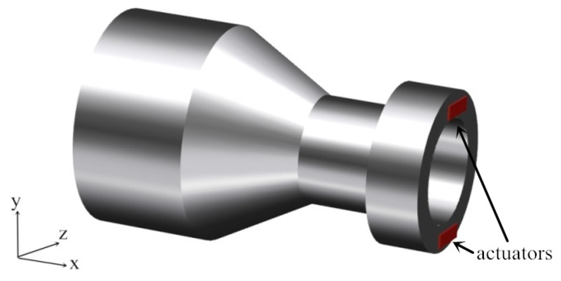
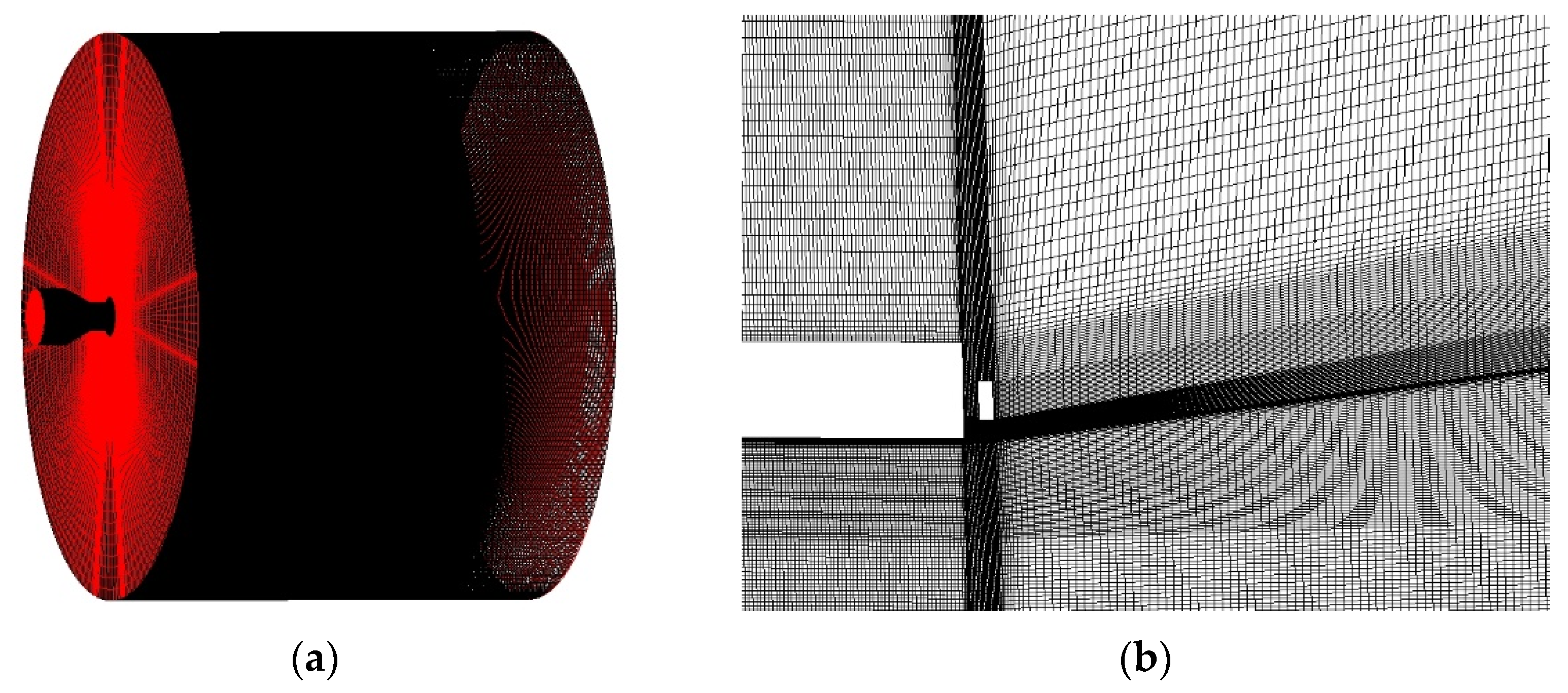
2. Computational Setup

The governing equations resolved in the current LES are the filtered incompressible Navier–Stokes equations:
u ¯ i x i = 0
u ¯ i t + u ¯ j u ¯ i x j = 1 ρ p ¯ x i + ν ( 2 u ¯ i x j 2 + 2 u ¯ i x i x j ) τ i j x j
where u ¯ i ( x i , t ) is the resolved velocity field and τ i j is the subgird stress tensor:
τ i j = u i u j ¯ u ¯ i u ¯ j
which is simulated by the eddy viscous model:
τ i j = 2 ν T S ¯ i j + 2 3 δ i j k s g s
where ν T = C k k s g s 1 / 2 Δ is the subgrid eddy viscosity, Δ is the filter width, ksgs denotes the subgrid kinetic energy and S ¯ i j = 1 2 ( u ¯ i x j + u ¯ j x i ) is the filtered strain rate tensor. In this work, the transport equation of ksgs is solved:
k s g s t + u ¯ j k s g s x j = τ i j u ¯ i x j ε + x i ( ( ν T + ν ) k s g s x i )
The dissipation rate is obtained by:
ε = C e k s g s 3 / 2 Δ
The model coefficients Ck and Ce are calculated by a dynamic procedure proposed by Kim and Menon [21]. The comparative studies of Fureby et al. [22,23] showed that this local dynamic one equation model is more tolerate for coarse grids and accurate for transition and unsteady flows.
The governing equations were discretized by the finite volume method. In the discretized equations, a second-order central difference scheme was used for the spatial terms, providing the least numerical dissipation. For the time discretization, the second-order Crank–Nicholson scheme was implemented. The above equations were solved by the PISO algorithm implemented as pisoFoam in the OpenFOAM.
A convergent nozzle with a pipe was used to produce the primary jet. Two slot-type fludic jet actuators were placed on opposite sides of the nozzle. The diameter of the nozzle exit was 4′′ and the length and width of the rectangle actuator exit were 1.7′′ and 0.08′′, respectively. Figure 1 shows their arrangement and the coordinate system. The origin of the coordinates is located at the center of nozzle exit. The computational domain was extended 15D in the streamwise direction from the nozzle exit and 10D in the radial direction from the centerline. LES is inherently grid-dependent due to its impact on the cutoff location within the spectrum of turbulence. Consequently, the multi-block approach was used to ensure higher mesh density at important regions, such as the nozzle wall boundary layer, jet shear layer and the region the primary jet and control jets interacted. The overall mesh and detailed mesh near the nozzle exit are shown in Figure 2. In the nozzle, the height of the first cell normal to the wall was set to keep y+ < 1 (approximately 0.00025D), ensuring a good boundary layer resolution. In the streamwise direction, the mesh was designed considering both the accuracy and cost. Near the nozzle entry, the length of the cell varied from 0.04D to 0.02D. In the converging part, the cell size was refined to 0.01D. To capture the transition of the boundary layer to shear layer, a relatively fine cell size of Δx/D = 0.0015 was used in the adjacent of the nozzle exit. Out of the nozzle, 600 cells were distributed in the streamwise direction, half of which were in the near field, resulting in a cell size equal to Δx/D = 0.02 at the end of the potential core (x/D = 5). In the azimuthal direction, 300 nodes were uniformly distributed, yielding a cell size of rΔθ/D = 0.01 at the nozzle exit. The radial grid length was 0.0005D at the lip of the nozzle exit and the resolution gradually decreased to 0.02D at r = 3D from the centerline. The total number of cells was about 40 million. In order to investigate the effect of mesh resolution on the results, a finer mesh with 1.5 times more cells in the shear layer and potential core region for the unforced jet was used. To validate the simulation result, Figure 3 compares the centerline and radial profiles of the time-averaged streamwise velocity between the cases with different mesh resolution and the available experimental data by Wickersham [13]. Uj is the bulk velocity at the nozzle exit and Uc is the time-averaged streamwise velocity along the centerline. The length of potential core is slightly overpredicted, but the decay rate of centerline velocity and radial profile are consistent with the experiment, which suggests the simulation can reasonably predict the jet development. The fine mesh case slightly improves the accuracy, but the difference is negligible. Considering the computing cost, the moderate mesh is employed in this study.
A uniform velocity without considering boundary layer and fluctuation was used at the nozzle entrance, resulting in bulk velocity Uj = 10 m/s at the nozzle outlet. For wall boundaries, the no-slip condition was used. Non-reflective boundary conditions implemented by solving a convective equation were employed at outflow. To allow entrainment at the circumferential boundary, free stream conditions were applied. The pulsed jet was achieved by switching the velocity magnitude from 0 to target value with a 0.5 duty cycle. The two pulsed jets are working with 180° phase difference. The amplitude of the pulsed jet was adjusted by the velocity magnitude of the actuator inlet.
The time step of each case was set to limit the maximum Courant number at approximately 0.5. The total solution ran for two phases. The first phase was carried out to allow the flow field fully developed and lasted 75 characteristic time (D/Uj). Subsequently, another 150 characteristic time was executed to do average and sample statistics.

3. Results and Discussion
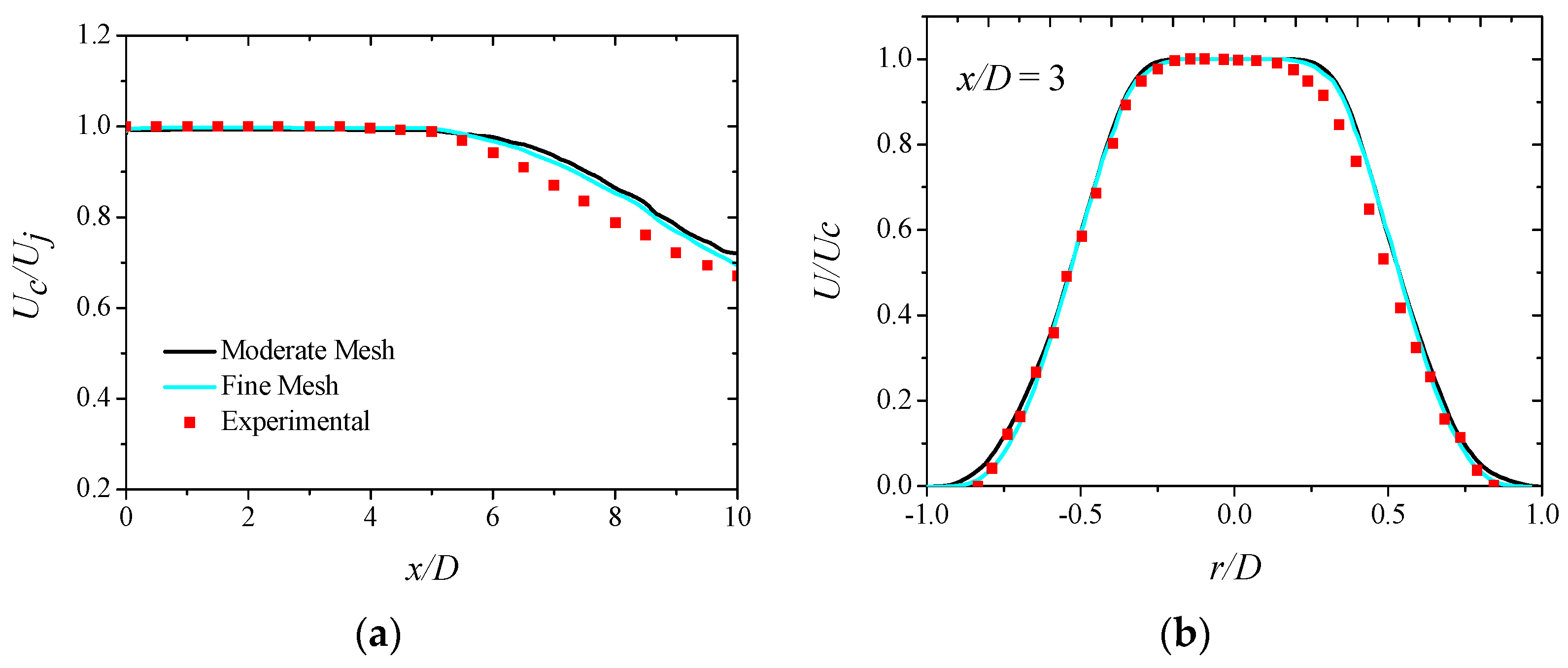
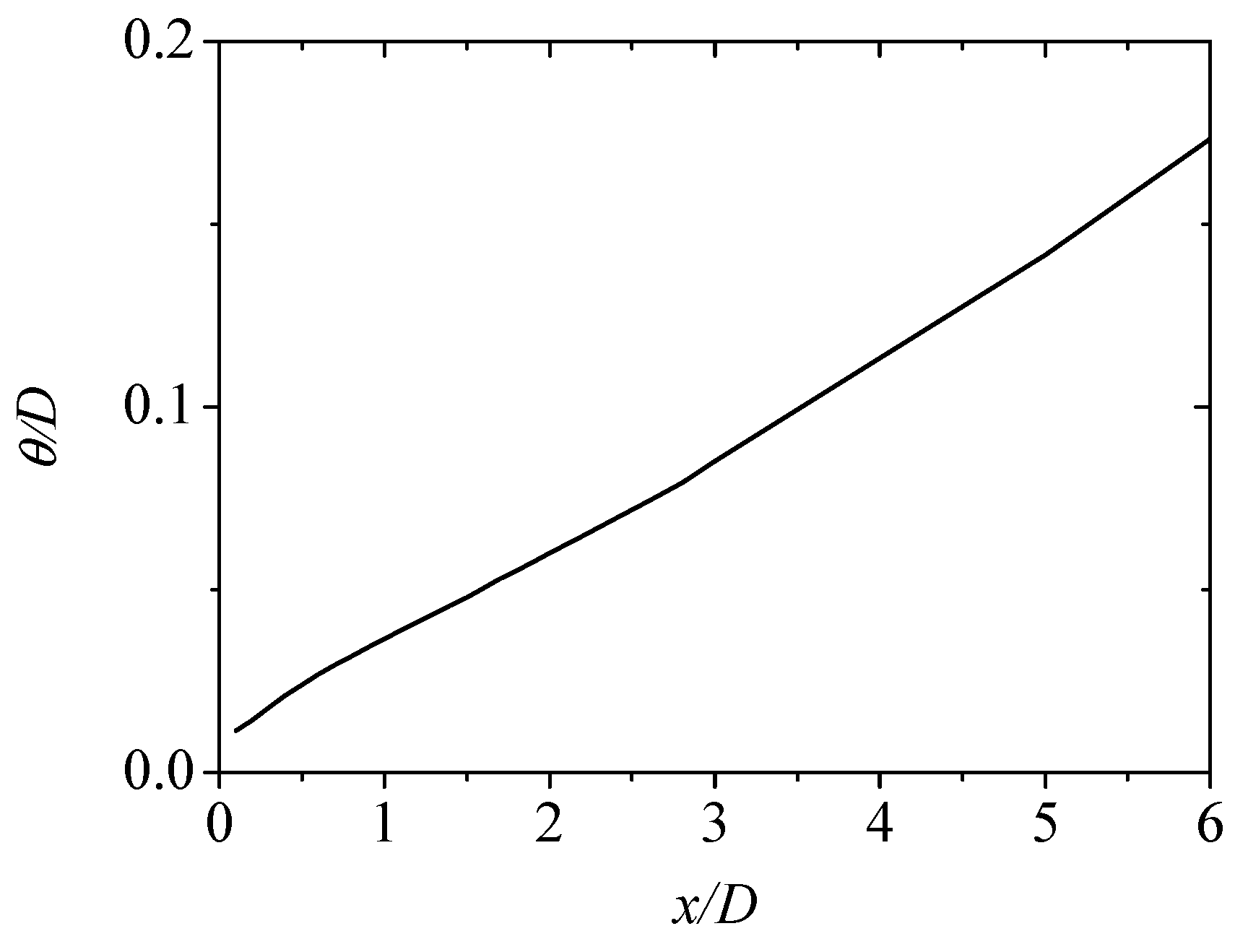
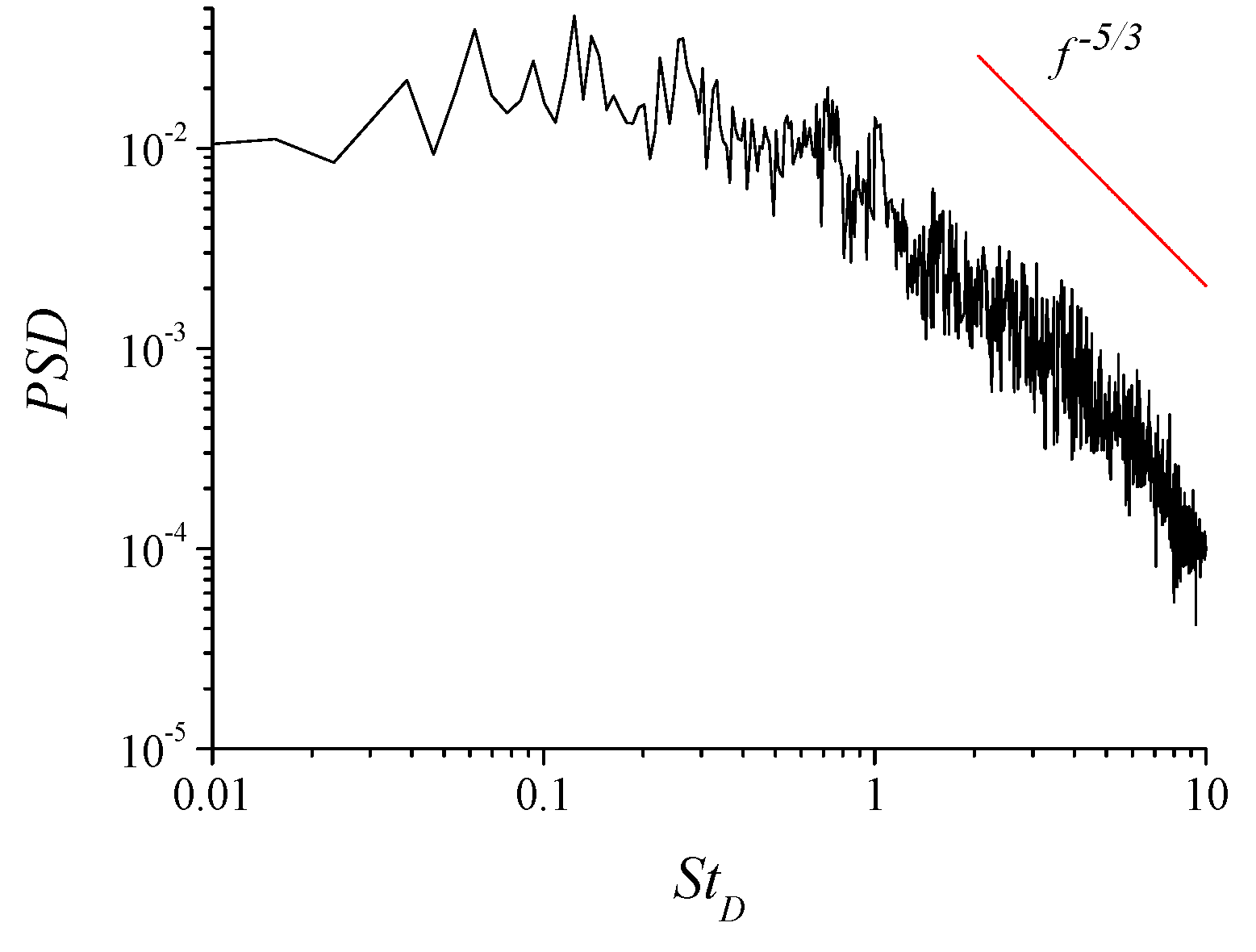
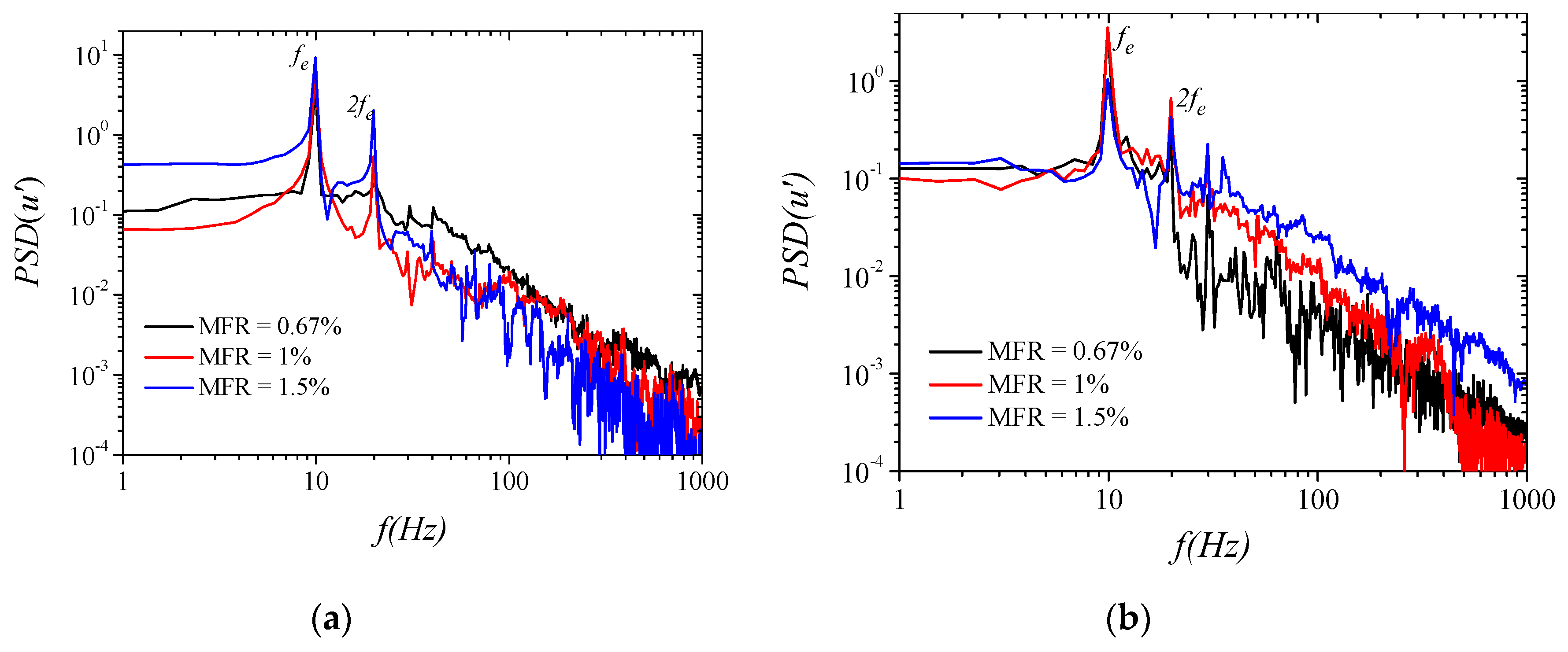
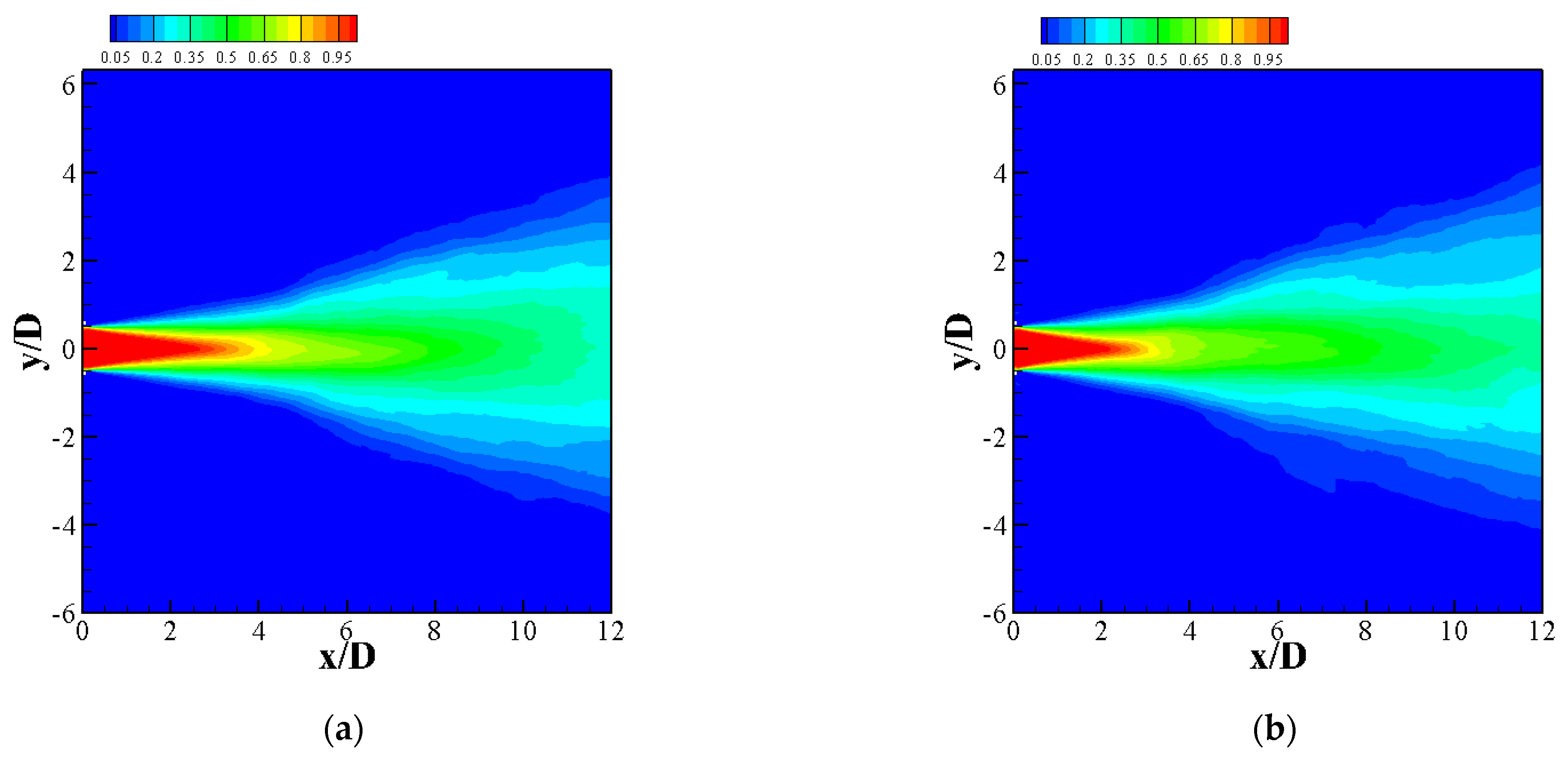
3.1. No Control

The unforced jet is introduced here briefly; more details can be found in previous work [20]. The boundary layer develops in the nozzle and reaches a nearly turbulent state at the nozzle exit. The momentum thickness of the initial shear layer is D/θ = 135; its shape factor is H = 1.52, which lies between the fully turbulent value (H = 1.3) and the laminar value (H = 2.6), while it is closer to the former one. The growth of the shear layer is investigated based on the development of momentum thickness θ in Figure 4. The momentum thickness is estimated from the mean streamwise velocity U as:
θ = 0 r 0.04 U U c ( 1 U U c ) d r
where r0.04 is the position where U = 0.04Uc. The momentum thickness for the initial laminar jet grows rapidly near the nozzle exit, after which the rate of growth decreases progressively [24,25]. Regarding the initial turbulent jet, the streamwise variation can be fitted with two straight lines and the slope of the second line is higher than that of the first line. The profile in Figure 3 resembles that of the initial turbulent jet, and the changeover of slopes is approximately at x/D = 3, but it is not distinct, as reported by Husain [24].
Figure 5 displays the coherent structures identified by the pressure iso-surface. The structures indicate a fully turbulent state with small scales, while no dominant direction could be distinguished in these vortices. Figure 6 illustrates the plot of the power spectral density (PSD) of streamwise velocity fluctuation velocity at x/D = 1 on the lip line. A broadband spectrum is observed and no dominant peak could be detected. The spectrum decay rate corresponds to the Kolmogorov −5/3 spectrum, indicating the existence of the inertial subrange.

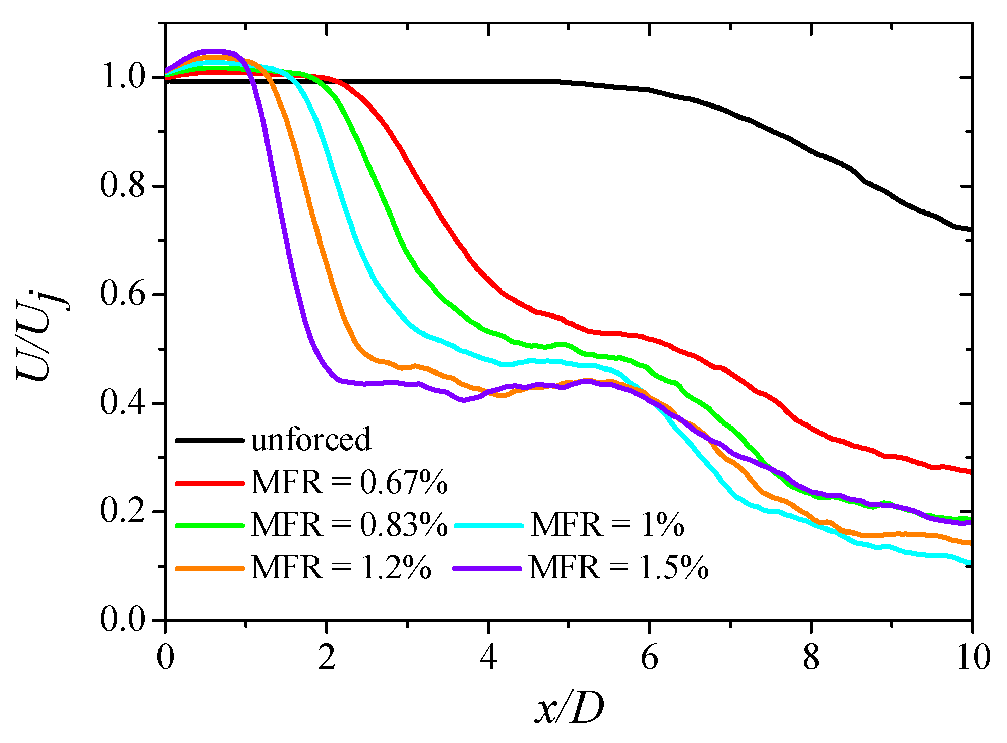
3.2. Forcing at Different Amplitudes

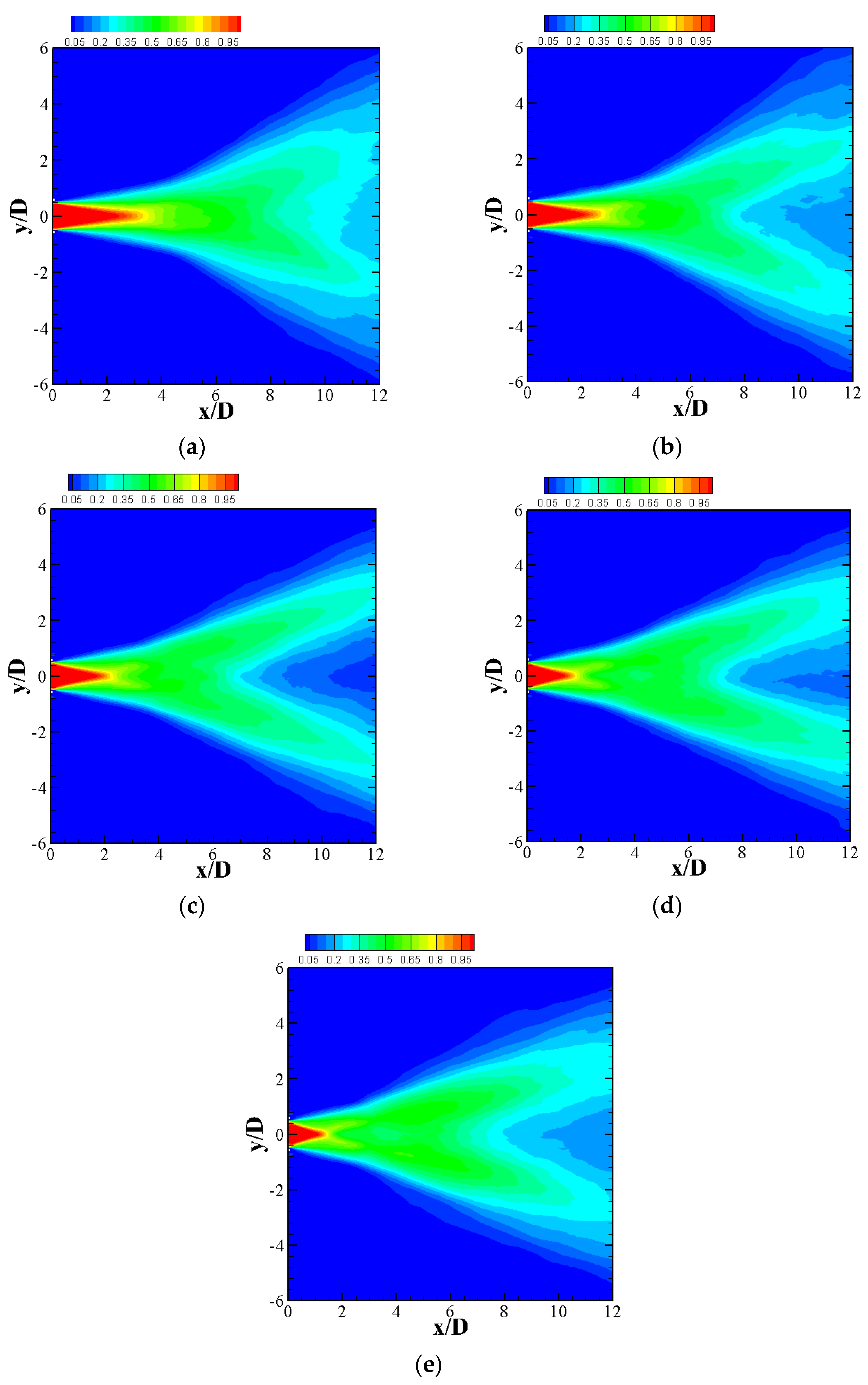
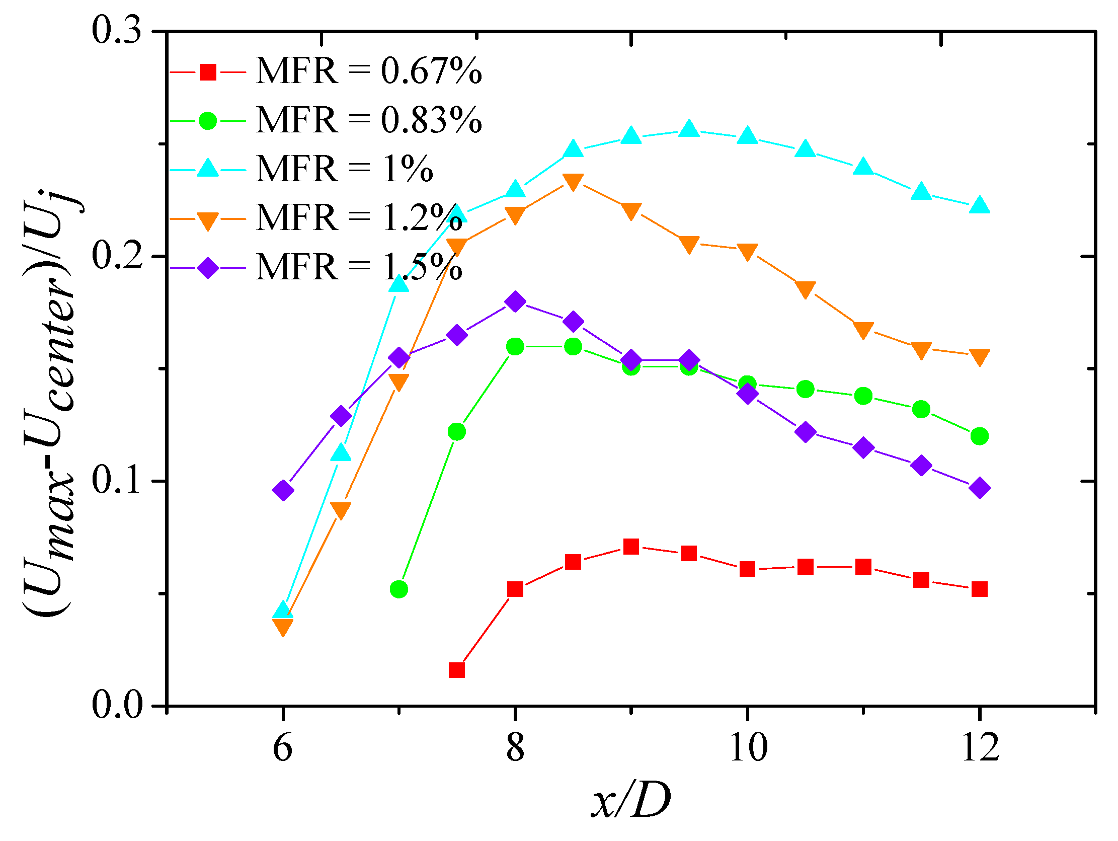
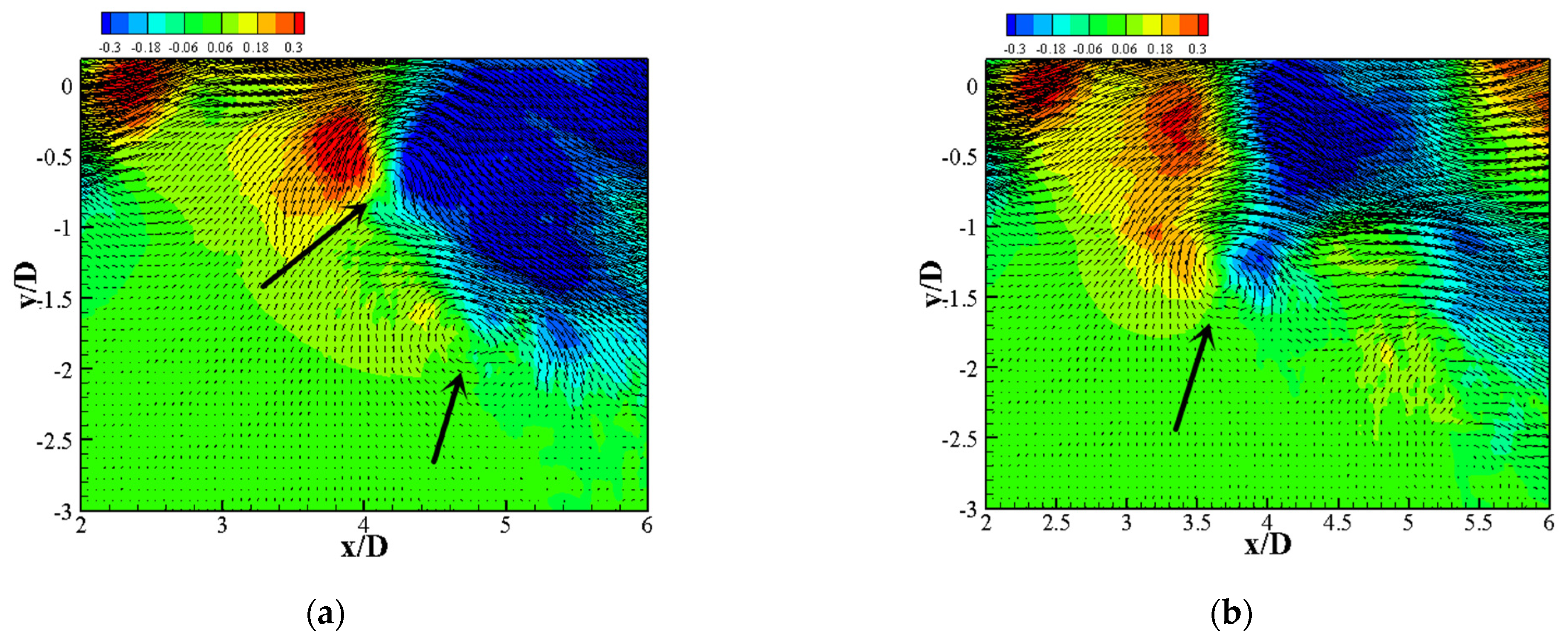
3.2.1. Effect on Mean Flow Field

At first, the velocity decay metric U*, defined as the ratio of the forced jet average velocity to the unforced jet average velocity at a downstream location of 10D along the centerline, i.e., U = U 10 D , f o r c e d U 10 D , u n f o r c e d , is used to evaluate the jet entrainment and spread. It has been proved that U* has direct relevance of jet entrainment and mixing [11,13,14]. Figure 7 shows the dependence of U* on MFR at StD = 0.1. At low MFR, U* decreases rapidly, implying a better mixing. When MFR is increased beyond 1%, it increases, suggesting an adverse impact on the control. Figure 8 shows the time-averaged streamwise velocity along the centerline for different amplitudes. The results exhibit a consistent trend. In particular, the velocity decays faster in the near field with increasing amplitude. However, beyond the x/D = 6 position, the MFR = 1% case displays the maximum velocity decay rate compared to the other cases. Figure 9 presents contours of the time-averaged streamwise velocity in the forced plane in order to examine the primary jets development. The results indicate that the jet shear layer spreads faster in the near field with increasing control jet amplitude. It could be noticed that, downstream, the jet splits into two branches, forming a bifurcating jet. Once the bifurcation has been established, two velocity peaks are displayed in bifurcation plane in radial direction and the jet separates as flows downstream. The spreading rate and mixing are significantly amplified [16]. Moreover, Figure 8 reveals that the forcing amplitude has a significant effect on jet bifurcation. When the MFR is below 1%, the jet bifurcates in the upstream with a larger angle with increasing amplitude, so the bifurcation is enhanced. However, when the MFR is further increased, the two branches tend to move towards each other, resulting in a smaller bifurcation angle. This variation trend is consistent with that of the U* depicted in Figure 8.
To quantify these observations, the jet half-width in the forced plane, defined as U(x, δ0.5, 0) = 0.5U(x, 0, 0), is plotted in Figure 10. The results illustrate that the MFR = 1% case exhibits the largest jet width downstream of x/D = 8. This is consistent with the distinct bifurcation that can be observed in Figure 9c. For an MFR higher than 1%, the jet width grows faster in the near field. However, downstream of x/D = 6, the spreading rate changes to a lower and more homogeneous value, indicating that the jet bifurcation is constrained. The difference between peaks and centerline velocities can be used to evaluate the strength of the bifurcation [26]. Figure 11 shows the strength of the bifurcation with different amplitudes. The results suggest that the jet bifurcated at an upstream location as the forcing amplitude increases. Then, the bifurcating strength decays in a nearly linear relationship with distance. It is remarkable that, at MFR = 1%, the jet exhibits the largest bifurcation strength and the slowest decrease of its magnitude. As can be seen in Figure 12, the radial location of the peak velocity also increases linearly with increasing streamwise location. The slope of the line can be defined as the bifurcation angle of the jet. Table 1 lists the bifurcation angles with different forcing amplitudes, confirming that forcing at MFR = 1% yields the largest bifurcation angle, while when the MFR of the pulsed jet is further increased; the effect on jet bifurcation is negative.

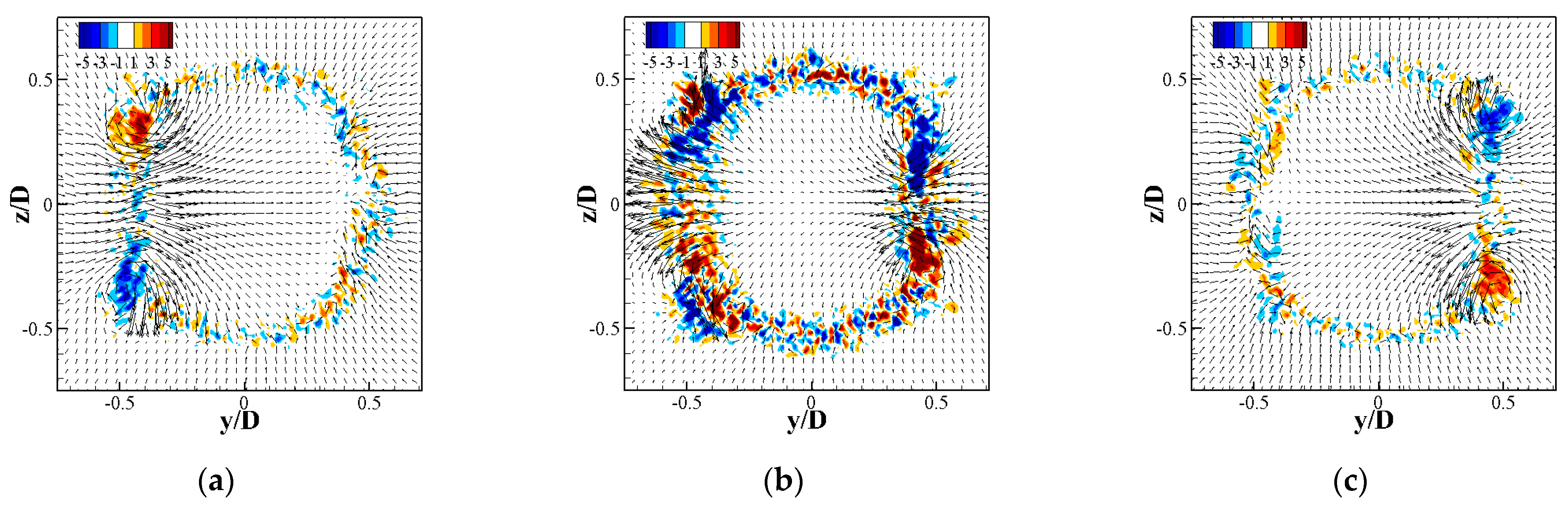
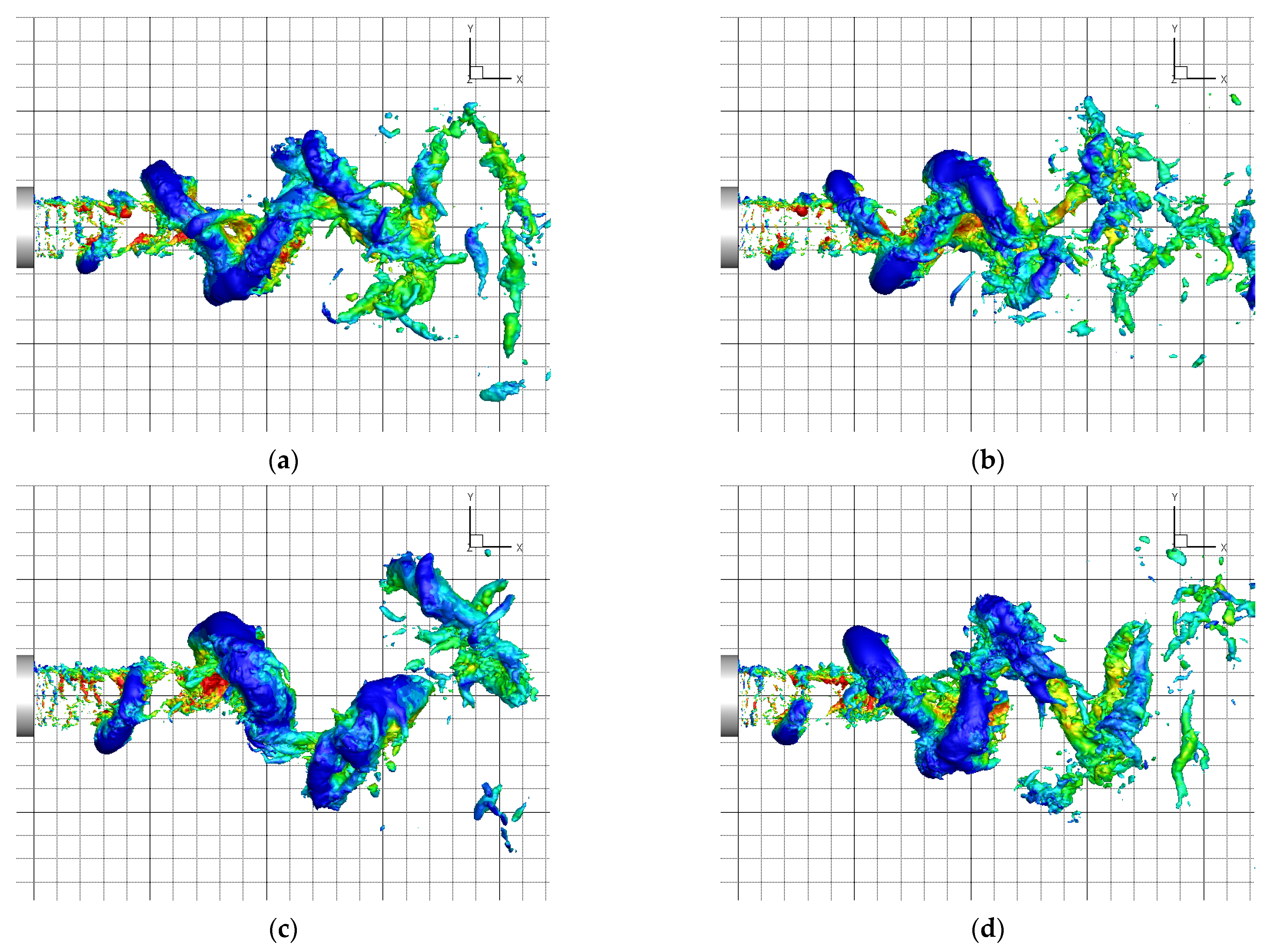
3.2.2. Effect on Azimuthal Structures

The mechanism of the bifurcating jet can be described as follows. The flapping perturbation promotes the generation of inclined vortex rings with uneven vorticity distribution. Consequently, the vortex rings have different self-induced velocities. When the induced radial velocity is large enough, the vortex rings alternatively separate, forming two distinct branches [16]. The experiment of Parekh et al. [27] revealed that the spreading angle increases dramatically with increasing excitation amplitude. They also mentioned that a saturation level in amplitude should be expected; however, this was not reached in the experiments. The observations of the present study prove the existence of an amplitude saturation value. This implies the existence of an unclear mechanism of bifurcating jet in this kind of forcing method, as the bifurcations are restrained at higher amplitudes. In order to further investigate these problems, the present work firstly focused on the large-scale vortex structures. Figure 13 displays the coherent structures in the flow field at the same phase in one forcing cycle. The length of the major grid is 2D in these figures. As reported in our previous study, inclined vortex fragments generated by the perturbation of the pulsed jets gradually grow in the azimuthal direction into full rings and then alternatively move to opposite directions in the downstream [20]. As the forcing amplitude increases, the vortex ring tends to be larger in scale and grows faster in the azimuthal direction. When the formation of the vortex tube begins, both ends have a smaller cross-section, which leads to a higher self-induced velocity compared to that at the middle part. In the downstream direction, the mutual interaction of neighboring rings promotes the inclination so that there is a larger radial velocity, ultimately resulting in the splitting of the primary jet [20,28]. According to Figure 13, when the azimuthal vortex structure grows into a full ring, it tends to tilt at a smaller angle with respect to the nozzle exit with increasing amplitude. This results in a smaller projection of the induced velocity in the radial direction, which has a negative effect on bifurcating.
In addition, the forcing amplitude also has a crucial impact on the strength of the azimuthal structures. To subtract large-scale structures from fine turbulence, the instantaneous velocity snapshots were processed using the proper orthogonal decomposition (POD) method, after which they were reconstructed with only the first few modes. This method has been introduced in our previous study [20]. In Figure 14, the vorticity in the near field of the forced plane is displayed. It can be observed that the vortices generated at higher forcing amplitudes have a larger vorticity magnitude and a less elliptical shape. These observations are related to the generation of the vortex. As explained in our previous study, the injection of the control jet induces a large negative velocity gradient ( V x ), which promotes the roll-up of the shear layer [20]. A higher forcing amplitude corresponds to a higher momentum ratio, which leads to deeper penetration in the primary jet and larger velocity gradient. Hence, the vortex is stronger and causes larger self-induced velocity in the near field, which has positive effect on jet bifurcation based on the mechanism of formation of bifurcating jet. Consequently, there is a balance of effects on vortex rings when the amplitude is increased, and apparently, the primary jet exhibits the largest bifurcation angle at medium amplitudes.
Figure 15 illustrates the spanwise vortices under different amplitudes further downstream. At this position, the vortex has grown into a full ring. The vorticity lumps with opposite signs in the shear layers are the cross-sectional plane of the vortex ring. Figure 15 also reveals that the vortex ring inclines less to the downstream with increasing forcing amplitude. While the upper part of the ring is located at the same place, the lower part is located at a further upstream position as the amplitude increases. It is also noteworthy that the vorticity magnitude at the lower shear layer is decreased at higher amplitudes. At the highest amplitude investigated in this study, the lower part of the vortex ring moves upstream of the upper part and the vortex becomes hardly discernible. This is the result of the stronger interaction between the streamwise vortex pair and the vortex ring, which will be discussed later in this paper.
The behavior of the azimuthal vortex can also be indicated by the PSD of the velocity fluctuation in the shear layer. The instantaneous velocity was collected at the lip line of the forced plane at different streamwise positions (y/D = 0.5, x/D = 2, 4). In Figure 16a, the peak value at forcing frequency fe implies that the vortex strength increases with increasing amplitude. This is consistent with the observations in Figure 14. When the spanwise structure evolves into a full ring, two rings go through the shear layer in a cycle; thus, the peak at 2fe emerges. At x/D = 2, this value is distinct at MFR = 1.5%, while it is hardly discernible at MFR = 0.67%. This result proves the difference in azimuthal growth rate of the spanwise structure that was observed in Figure 13. In the downstream, the peak values at MFR = 1% become the largest, which indicates that the coherence of the vortex ring is impaired at higher amplitudes.

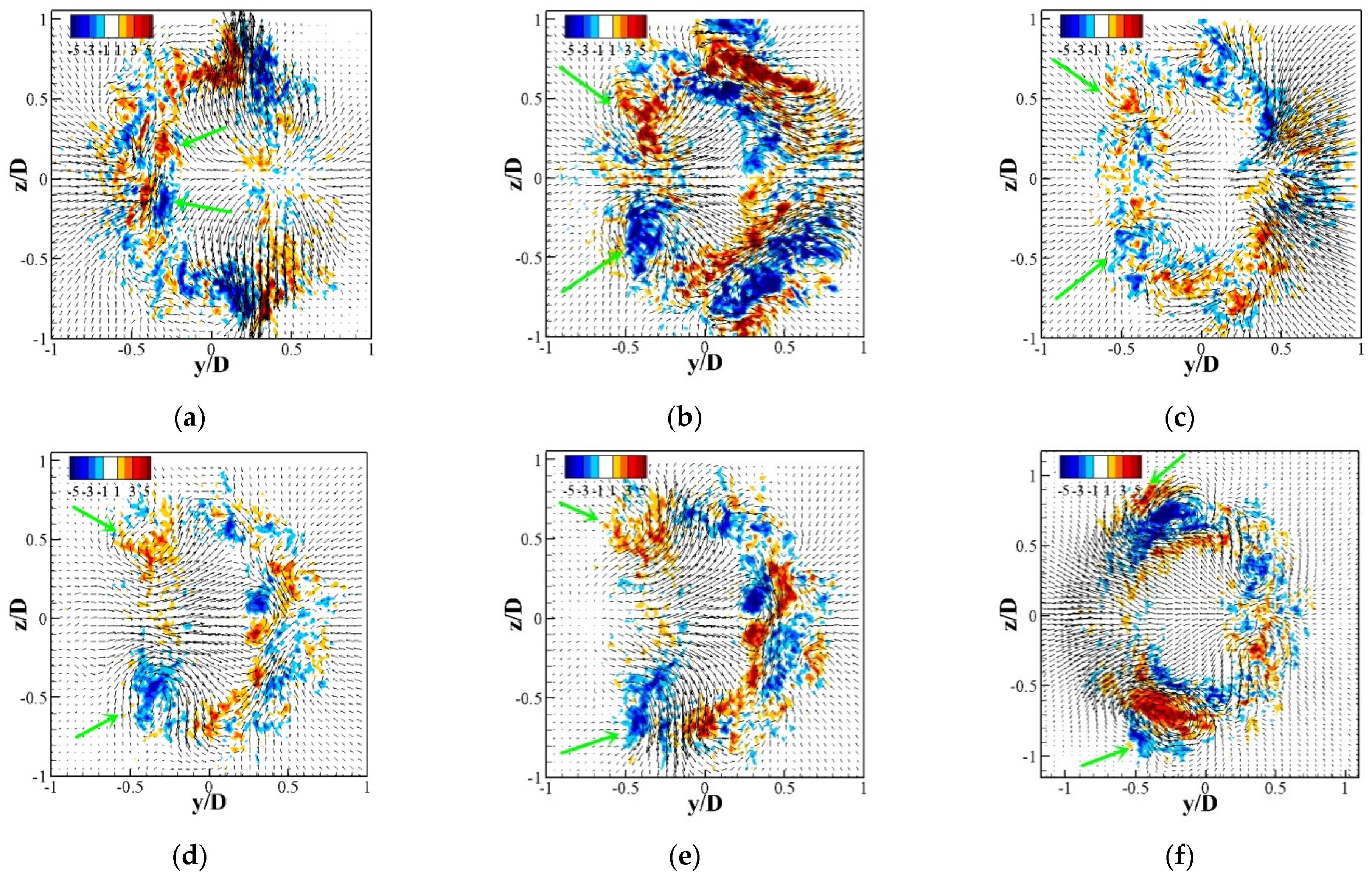
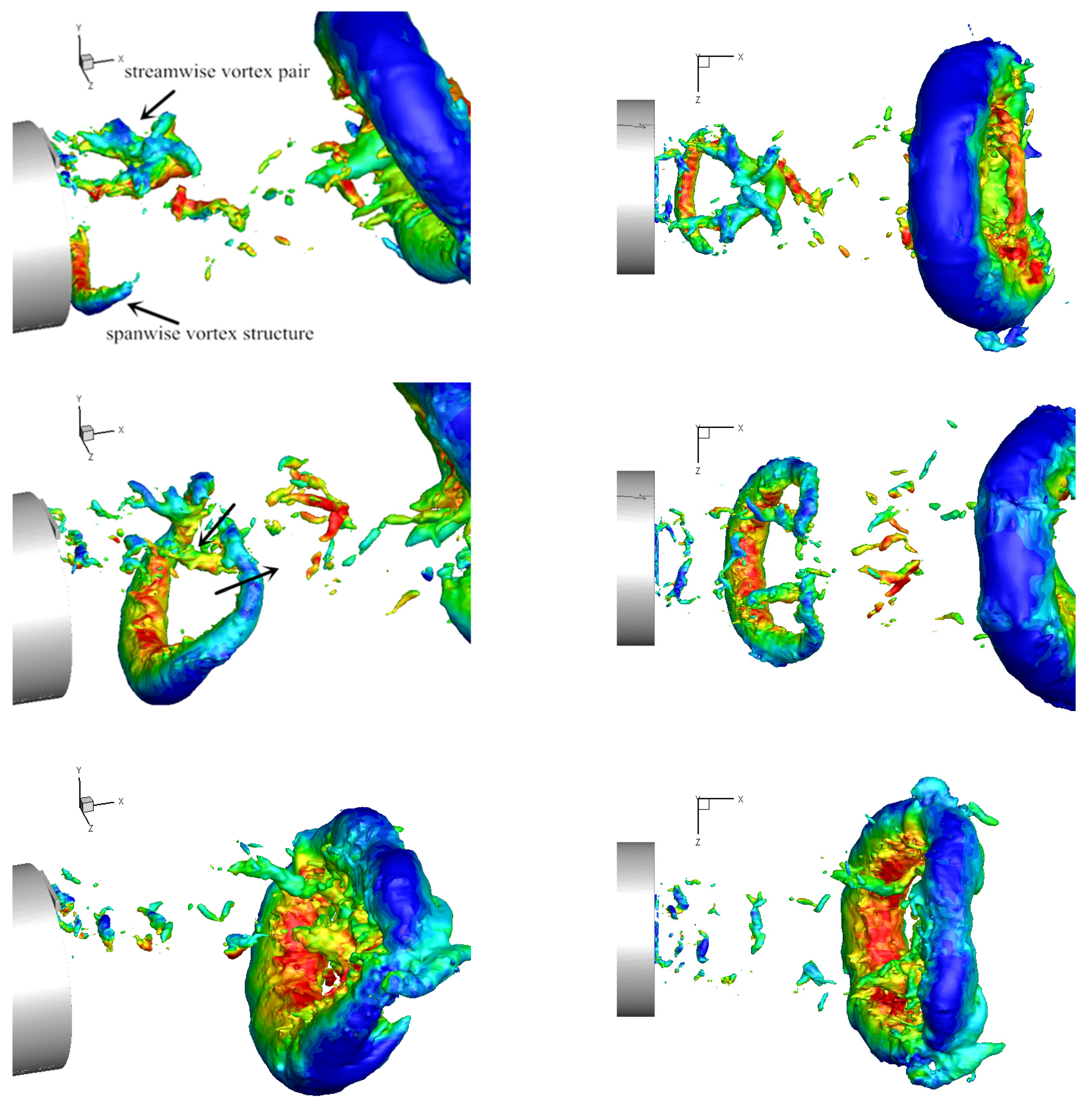
3.2.3. Effect on Streamwise Structures

When the azimuthal structures grow in the azimuthal direction, they interact with the structures produced by the control jets. Figure 13 illustrates that these structures are a leading vortex followed by a counter-rotating vortex pair (CVP) in the braid region, and are formed by the deflection of the secondary flow [29]. It is believed that the interaction between streamwise structures and titled vortex rings makes the rings less inclined. In order to investigate the behavior of the CVP, the instantaneous streamwise vorticity in fixed cross-sectional planes was acquired over a series time sequence to reflect the passage of the streamwise vortex structures. The original flow field is also processed by POD. The streamwise vorticity and in-plane velocity vectors of the MFR = 0.67% case at x/D = 0.5 are demonstrated in Figure 17. At t = 0, the control jet on the y-direction suspends the ejection and the control jet at the opposite side begins to work. The CVP produced during the previous period remains around (−0.5D, ±0.4D). Then, at t = 0.125 T, another CVP emerges with larger vorticity, which is the front part of the streamwise vortex tubes. At the same time, the CVP at the y-direction disappears, since it has convected downstream. At t = 0.5 T, the vortex structure is similar to that in the beginning, but it is actually a mirror image. It can be deduced that the front parts of the two vortex tubes are closer than their tail parts. In this plane, the structure of the vortex is simple, since the tilted azimuthal vortex near the nozzle exit is still small and does not interact with the CVPs. Figure 18 illustrates the development process of the CVP at the x/D = 2 plane. Figure 18a is the moment when the front part of the CVP in y-direction interacts with the inclined vortex ring, which has been produced by the control jet in the y-direction. It can be seen that the CVP is located at approximately (−0.3D, ±0.2D), and penetrates deeper into the primary jet. This is attributed to that the front part of the tilted vortex ring (in the y-direction) has inward induced velocity, inhaling the CVP into its interior. As the vortex ring moves downstream, the inward induction becomes weaker, causing the CVP to gradually separate in a further radial position with larger size. It should be mentioned that the lump of vorticity in the elliptic shape in Figure 18b is the projection of the rear part of the tilted ring on the cross-sectional plane. When the vortex ring leaves the plane, it induces a large velocity in the y-direction, which is adverse to that of the CVP. This weakens the CVP significantly and makes it difficult to be distinguished (Figure 18c). As the vortex ring moves further downstream, its adverse effect on the CVP is diminished, while the next vortex ring arrives at the x/D = 2 plane. This vortex ring is behind the CVP; thus, its outward induced velocity makes the CVP to gradually separate. This can be observed in Figure 18d,e, where the distance between the two streamwise vortices increases evidently. Moreover, the occurrence of other CVPs in the y+ direction can be observed at (0.3D, ±0.2D). In Figure 18f, the CVP, entirely separated, has smaller size and magnitude and is located around (−0.5D, ±0.9D). It shows that the tails of the streamwise vortex tubes are attached on the outer surface of the vortex ring. The location is determined by the balance between its induced inward velocity and the outward velocity induced by the azimuthal vortical structure. The dynamics of the CVP are very similar to that of the streamwise structures formed due to the azimuthal instabilities in the braid region, at which the downstream portions are pulled inside the jet, while the upstream parts are stretched outwards and then wrapped around the vortex ring [6,30].
In Figure 19, the time-averaged streamwise vorticity at the x/D = 0.5 cross-sectional plane at the three different amplitudes is presented in order to investigate the effect of forcing amplitude on the streamwise structures. At higher amplitudes, the streamwise vortices have a larger size and penetrate deeper into the primary jet. The vorticity magnitude also increases significantly. Therefore, the entrainment of the CVP becomes stronger, leading to a faster spread of the primary jet in the near field (Figure 11). Consequently, the strength of the mutual induction between streamwise and azimuthal structures is also enhanced.

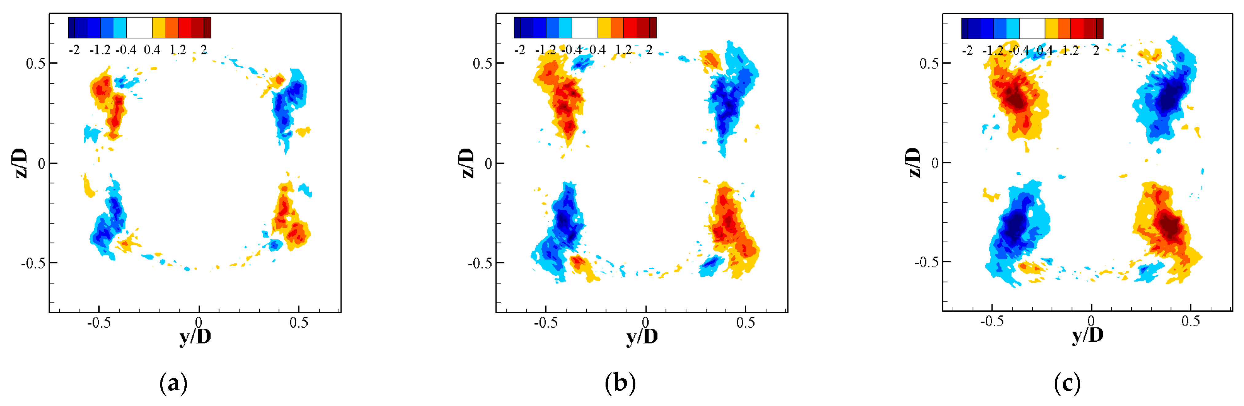
3.2.4. Mutual Interaction

As mentioned above, the mutual interaction between vortex rings and streamwise structures reduces the inclination angle of the vortex ring, which has a negative effect on jet bifurcation. In order to clearly observe the critical process, the evolution of these three-dimensional structures is visualized by iso-surfaces of pressure in Figure 20. In the first image, the upper control jet has just been activated. A streamwise vortex pair has formed, and at the opposite side, the resulting azimuthal vortex fragment with both ends inclined downstream is visible. Since the size of the azimuthal vortex is still small, it does not interact with the streamwise vortex pair at this time point. As these structures move downstream, the streamwise vortex pair penetrates deeper into the primary jet and the spanwise structure grows along the azimuthal direction. When these structures interact, the large inward induced velocity between the two streamwise vortices pulls the azimuthal structures towards the center of the jet. At the same time, out of the streamwise vortices, the induced velocity pushes the vortex ring to larger radial place and broadens the front part of the ring. In addition, this effect makes this part of the ring to move further away from the high-speed region of jet, lowering its convection velocity. Since the leading parts of the streamwise vortices are inclined towards the primary jet, these vortices also drag the front part of the vortex ring backwards. These combined effects undulate the vortex ring, increasing its shape complexity. Consequently, the leading part of the vortex ring is gradually pulled back, and the inclination is decreased. Moreover, some induced streamwise vortices are generated at the position where the ring has been folded, and can be clearly observed in the last image. The induced structures are very similar to those formed at the corners of a rectangular jet [31]. According to the discussion on Figure 19, as the forcing amplitude increases, the strength of the streamwise vortices increases significantly, after which the effect of mutual interaction on the vortex ring becomes stronger. As a result, the inclination of vortex ring is restrained (Figure 13).

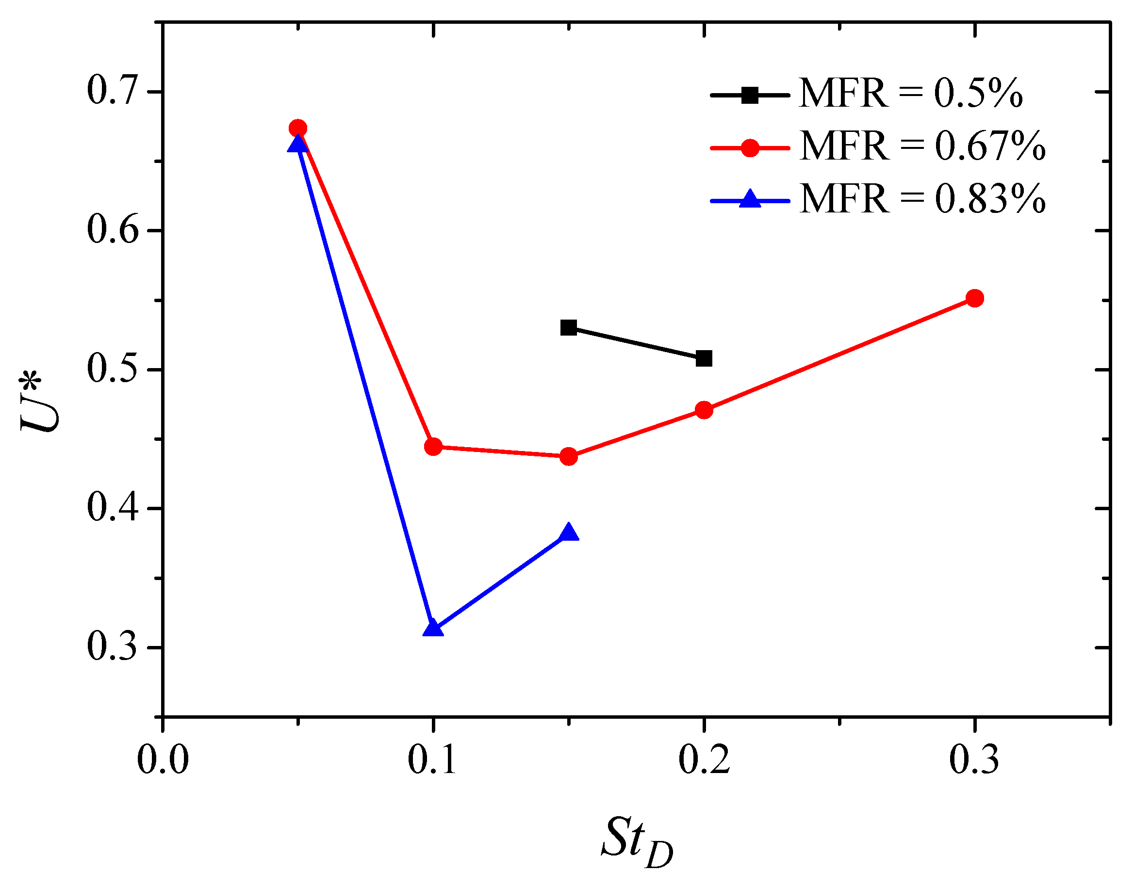
3.3. Coupling Effect of the Forcing Frequency and Amplitude

The forcing frequency is one of the most important parameters in the pulsed jet flow control method. Previous studies have shown that the major effect of the forcing frequency mainly affects the streamwise spacing between two successive vortex rings [20]. At low frequencies, although each ring can grow to a larger size, the mutual induction between two neighboring rings is very weak, since the distance between them is large. At high frequencies, the vortex structures are closely spaced; thus, each vortex is of a small size. The structures interact near the nozzle exit before evolving to full vortex rings. Hence, the mutual induction is also not strong. At the optimal frequency, the vortex rings are well arranged, and the front part of a full ring can be pulled into the rear part of the preceding ring. This causes a strong mutual interaction that significantly increases the inclination of these two rings. Consequently, the jet bifurcates further downstream. In addition, as thoroughly explained in the previous subsection, the forcing amplitude also affects the evolution of the vortex structures. Therefore, there must be a coupling effect between these two factors. This has been previously discussed in the study by Wickersham [13].
In order to investigate and verify this phenomenon, some additional simulations with various combinations of frequencies and amplitudes were carried out, and the centerline velocity decay metric U* is displayed in Figure 21. These results confirm that the optimal frequency with regard to centerline velocity decay rate decreases with an increasing forcing amplitude. When the forcing amplitude is low, the optimal frequency is within the range of the preferred mode frequency of an unforced jet (StD = 0.2~0.6, which varies for different initial conditions). At high amplitudes, the optimal frequency converges to approximately 0.1. This can be inferred from the fact that the value of U* increased abruptly when StD decreased from 0.1 to 0.05, regardless of the forcing amplitude. One possible explanation for the shift of the optimal frequency may be the following. When the forcing amplitude increases, the azimuthal vortex has a higher vorticity magnitude and grows faster in the azimuthal direction. Therefore, the interaction between the successive structures will occur earlier compared to that at a lower forcing amplitude. The upstream half of a preceding vortex ring, which is stronger, will engulf the front half of a newly generated vortex structure before it develops to a full ring. In this case, the intensive mutual induction between these two structures, which is crucial for the off-centerline movement of the vortex ring, would not happen. A lower forcing frequency would result in a long distance between two neighboring vortex rings, preventing the weaker part of the succeeding ring being engulfed by the preceding one. Consequently, a slip-through motion between the two full vortex rings will take place. Due to the induction, the weaker half of the upstream vortex ring is inhaled and slips through the stronger part of the preceding vortex. During this process, the preceding vortex is pulled to outward and becomes more inclined. Consequently, a large off-centerline velocity is produced by these two vortices [28].
To illustrate this, the coherent structures under different amplitudes and frequencies are displayed in Figure 22. When the MFR is 0.67%, the vortex ring is stronger and more complete at the location where mutual induction occurs at StD = 0.15, which is the optimal frequency at this forcing amplitude. When the amplitude is increased to 0.87%, the vortex becomes stronger and larger in size. The two vortices mentioned above coalesce to a larger one. While the StD is reduced to 0.1, which is the optimal frequency at this forcing amplitude, the two vortices become more separated and inclined, indicating vigorous induced velocity between them. Figure 23 shows the radial velocity at this moment, the arrows point to the vortices. This result is consistent with the interpretation of Figure 22. Concerning the saturation of the optimal frequency at higher amplitudes, two main reasons may be responsible. First, when the frequency is further decreased, the distance of two neighboring vortex rings is too far to result in intensive induction. The slight oscillation of the primary jet attributes to the initial inclination of the vortex ring. Second, at higher amplitudes, the streamwise vortex pair plays an important role in pulling the vortex backwards, which also makes the vortices less inclined. The time-averaged streamwise velocity contours for StD = 0.05 at two different amplitudes are displayed in Figure 24. It can be seen that, under these conditions, these jets do not bifurcate at all and are very similar to an unforced jet.

4. Conclusions

In the present work, a turbulent jet controlled by two pulsed jets operating at a flapping mode was investigated using LES. The effect of forcing amplitude has been investigated in detail. Moreover, the coupling effect of forcing frequency and amplitude has also been discussed.
According to the results of this study, it has been found that the forcing amplitude has a significant effect on jet development. As the amplitude increases, the primary jet bifurcates at a further upstream position with a larger angle. At MFR = 1%, the jet exhibits two distinct branches with the largest angle. When the forcing amplitude is further increased, the two branches tend to approach each other. This phenomenon is attributed to by the effect of amplitude on the streamwise vortex pair and azimuthal vortex ring. As the amplitude is increased, the streamwise vortex pair increases in strength and penetrates in primary jet deeper. The front part of the streamwise vortex pair is inhaled into the inner part of the preceding vortex ring, while its tail is pushed outwards and is then wrapped on the outer surface of the following vortex ring. The front part of the streamwise vortex drags the front half of the preceding vortex ring backwards. This makes the vortex ring less inclined, and thus, it impacts on the jet bifurcation. Meanwhile, higher forcing amplitudes can generate a vortex ring with larger vorticity and size. This leads to a more uneven distribution of vorticity, which promotes the jet bifurcation. These combined effects indicate in the existence of optimal forcing amplitude that the jet bifurcates and spreads the most.
The coupling effect of forcing amplitude and frequency is also investigated. The results demonstrate that the optimal frequency with regard to mixing efficiency decreases with increasing amplitude and saturates at larger amplitude. At the optimal frequency, two successive vortex rings have an intensive mutual induction, which causes the primary jet to bifurcate and spread rapidly. When the amplitude increases, the interaction occurs earlier before the succeeding vortex develops to a full ring, impairing the effect of mutual induction on the vortices. A lower frequency is needed to enlarge the space between neighboring rings so that the vortex structures can recover to optimal pattern. The saturation of the optimal frequency is related to the too large distance between neighboring rings and the increasing effect of the streamwise vortex pair, which inhibits the mutual induction.

Author Contributions

Conceptualization, Q.E. and B.K.; methodology, B.K.; software, B.K.; validation, W.D.; formal analysis, B.K.; investigation, W.D.; resources, W.D.; data curation, W.D.; writing—original draft preparation, Q.E.; writing—review and editing, B.K.; visualization, W.D.; supervision, B.K.; project administration, Q.E.; funding acquisition, Q.E. All authors have read and agreed to the published version of the manuscript.

Funding

This research was funded by the National Natural Science Foundation of China grant number [11572027]. And the APC was funded by the National Natural Science Foundation of China.

Acknowledgments

The authors are grateful to the National Supercomputer Center in Tianjin (NSCC-TJ), where the computations were carried on.

Conflicts of Interest

The authors declare no conflict of interest.

Nomenclature

MFRMass flow ratio
CVPCounter-rotating vortex pair
faAxial frequency, Hz
fhHelical frequency, Hz
StStrouhal number
LESLarge-eddy simulation
uVelocity, m/s
ρDensity, kg/m3
pPressure, pascal
νViscosity, m2/s
τijSubgird stress tensor
νTSubgrid eddy viscosity, m2/s
ΔFilter width
ksgsSubgrid kinetic energy
S ¯ i j Filtered strain rate tensor
εDissipation rate
DNozzle exit diameter
y+Wall Y plus
UjBulk velocity, m/s
UcTime-averaged streamwise velocity, m/s
HShape factor
θMomentum thickness
UMean streamwise velocity, m/s
PSDPower spectral density
U*Velocity decay metric
PODProper orthogonal decomposition
feForcing frequency, Hz

References

  1. Banken, G.J.; Cornette, W.M.; Gleason, K.M. Investigation of infrared characteristics of three generic nozzle concepts. In Proceedings of the 16th AIAA/SAE/ASME Joint Propulsion Conference, Hartford, CT, USA, 30 June–2 July 1980; p. AIAA-80-1160. [Google Scholar]
  2. Castelain, T.; Sunyach, M.; Juvé, D.; Béra, J.C. Jet-Noise Reduction by Impinging Microjets: An Acoustic Investigation Testing Microjet Parameters. AIAA J. 2008, 46, 1081–1087. [Google Scholar] [CrossRef] [Green Version]
  3. Behrouzi, P.; McGuirk, J.J. Flow Control of Jet Mixing Using a Pulsed Fluid Tab Nozzle. In Proceedings of the 3rd AIAA Flow Control Conference, San Francisco, CA, USA, 5–8 June 2006. [Google Scholar]
  4. Cattafesta, L.N.; Sheplak, M. Actuators for Active Flow Control. Annu. Rev. Fluid Mech. 2011, 43, 247–272. [Google Scholar] [CrossRef] [Green Version]
  5. Crow, S.C.; Champagne, F.H. Orderly structure in jet turbulence. J. Fluid Mech. 1971, 48, 547–591. [Google Scholar] [CrossRef]
  6. Liepmann, D.; Gharib, M. The role of streamwise vorticity in the near-field entrainment of round jets. J. Fluid Mech. 1992, 245, 643–668. [Google Scholar] [CrossRef] [Green Version]
  7. Zaman, K.B.M.Q.; Hussain, A.K.M.F. Vortex pairing in a circular jet under controlled excitation. Part 1: General jet response. J. Fluid Mech. 1980, 101, 449–491. [Google Scholar]
  8. Tamburello, D.A.; Amitay, M. Active control of a free jet using a synthetic jet. Int. J. Heat Fluid Flow 2008, 29, 967–984. [Google Scholar] [CrossRef]
  9. Ioannou, V.; Laizet, S. Numerical investigation of plasma-controlled turbulent jets for mixing enhancement. Int. J. Heat Fluid Flow 2018, 70, 193–205. [Google Scholar] [CrossRef]
  10. Kamran, M.A.; McGuirk, J.J. Unsteady Predictions of Mixing Enhancement with Steady and Pulsed Control Jets. AIAA J. 2015, 53, 1262–1276. [Google Scholar] [CrossRef] [Green Version]
  11. Parekh, D.E.; Kibens, V.; Glezer, A.; Wiltse, J.M.; Smith, D.M. Innovative Jet Flow Control: Mixing Enhancement Experiments. In Proceedings of the 34th Aerospace Sciences Meeting and Exhibit, Reno, NV, USA, 15–18 January 1996; AIAA: Reston, VA, USA, 1996; p. 308. [Google Scholar]
  12. New, T.H.; Tay, W.L. Effects of cross-stream radial injections on a round jet. J. Turbul. 2006, 7, N57. [Google Scholar] [CrossRef]
  13. Wickersham, P. Jet Mixing Enhancement by high amplitude pulsed fluidic actuation. Ph.D. Thesis, Georgia Institute of Technology, Atlanta, GA, USA, 2007. [Google Scholar]
  14. Yang, H.; Zhou, Y. Axisymmetric jet manipulated using two unsteady minijets. J. Fluid Mech. 2016, 808, 362–396. [Google Scholar] [CrossRef]
  15. Perumal, A.K.; Zhou, Y. Parametric study and scaling of jet manipulation using an unsteady minijet. J. Fluid Mech. 2018, 848, 592–630. [Google Scholar] [CrossRef]
  16. Reynolds, W.C.; Parekh, D.E.; Juvet, P.J.D.; Lee, M.J.D. Bifurcating and blooming jets. Annu. Rev. Fluid Mech. 2003, 35, 295–315. [Google Scholar] [CrossRef] [Green Version]
  17. Lee, M.; Reynolds, W.C. Bifurcating and blooming jets at high Reynolds number. In Proceedings of the 5th Symposium on Turbulent Shear Flows, New York, NY, USA, 7–9 August 1985. [Google Scholar]
  18. Danaila, L.; Boersma, B.J. Direct numerical simulation of bifurcating jets. Phys. Fluids 2000, 12, 1255. [Google Scholar] [CrossRef]
  19. Da Silva, C.B.; Métais, O. Vortex control of bifurcating jets: A numerical study. Phys. Fluids 2002, 14, 3798. [Google Scholar] [CrossRef]
  20. Kong, B.; Li, T.; Qitai, E. Large eddy simulation of turbulent jet controlled by two pulsed jets: Effect of forcing frequency. Aerosp. Sci. Technol. 2019, 89, 356–369. [Google Scholar] [CrossRef]
  21. Kim, W.W.; Menon, S. A new dynamic one-equation subgrid-scale model for large eddy simulations. In Proceedings of the 33rd Aerospace Science Meeting and Exhibition, Reno, NV, USA, 9–12 January 1995. [Google Scholar]
  22. Fureby, C.; Tabor, G.; Weller, H.; Gosman, A.D. A Comparative Study of Sub Grid Scale Models in Homogeneous Isotropic Turbulence. Phys. Fluids 1997, 9, 1416–1429. [Google Scholar] [CrossRef]
  23. Fureby, C.; Gosman, A.D.; Tabor, G.; Weller, H.G.; Sandham, N.; Wolfshtein, M. Large Eddy Simulation of Turbulent Channel Flows. 1997. Available online: https://citeseerx.ist.psu.edu/viewdoc/download?doi=10.1.1.45.5126&rep=rep1&type=pdf (accessed on 27 December 2021).
  24. Husain, Z.D.; Hussain, A.K.M.F. 1979 Axisymmetric mixing layer: Influence of the initial and boundary conditions. AIAA J. 1979, 17, 48–55. [Google Scholar] [CrossRef]
  25. Bogey, C.; Bailly, C. Influence of nozzle-exit boundary-layer conditions on the flow and acoustic fields of initially laminar jets. J. Fluid Mech. 2010, 663, 507–538. [Google Scholar] [CrossRef] [Green Version]
  26. Tyliszczak, A.; Geurts, B.J. Parametric Analysis of Excited Round Jets–Numerical Study. Flow Turbul. Combust 2014, 93, 221–247. [Google Scholar] [CrossRef] [Green Version]
  27. Parekh, D.E.; Reynolds, D.E.; Mungal, M.G. Bifurcation of round air jets by dual-mode acoustic excitation. In Proceedings of the 25th AIAA Aerospace Sciences Meeting, Reno, NV, USA, 12–15 January 1987. [Google Scholar]
  28. Suzuki HKasagi, N.; Suzuki, Y. Active control of an axisymmetric jet with distributed electromagnetic flap actuators. Exp. Fluids 2004, 36, 498–509. [Google Scholar] [CrossRef]
  29. New, T.H.; Tay, W.L. Cross-Stream Radial Fluid Injection into a Round Jet. In Proceedings of the 2nd AIAA Flow Control Conference, Portland, OR, USA, 28 June–1 July 2004. [Google Scholar]
  30. Grinstein, F.F.; Gutmark, E.J.; Parr, T.P.; Hanson-Parr, D.M.; Obeysekare, U. Streamwise and spanwise vortex interaction in an axisymmetric jet. A computational and experimental study. Phys. Fluids 1996, 8, 1515. [Google Scholar] [CrossRef]
  31. Gohil, T.B.; Saha, A.K.; Muralidhar, K. Direct numerical simulation of free and forced square jets. Int. J. Heat Fluid Flow 2015, 52, 169–184. [Google Scholar] [CrossRef]
Figure 1. Nozzle and actuators arrangements.
Energies 15 00640 g001
Figure 2. Computational mesh of (a) the overall domain and (b) the axial near the nozzle exit.
Energies 15 00640 g002
Figure 3. Comparison of the time-averaged axial velocity profile between the simulation and experiment (a) along the centerline [20] ad (b) along the radial direction at x/D = 3.
Energies 15 00640 g003
Figure 4. Streamwise variation of the shear layer momentum thickness.
Energies 15 00640 g004
Figure 5. Coherent structures of the unforced jet, visualized by the iso-surface of pressure and colored by the streamwise velocity magnitude, p/ρUj2 = −0.03.
Energies 15 00640 g005
Figure 6. Power spectral density of the streamwise velocity fluctuation at x/D = 1, y/D = 0.5.
Energies 15 00640 g006
Figure 7. Velocity decay metric U* for different amplitudes.
Energies 15 00640 g007
Figure 8. Decay of the time-averaged streamwise velocity along the centerline for different amplitudes.
Energies 15 00640 g008
Figure 9. Time-averaged streamwise velocity in the forced plane, normalized by Uj. (a) MFR = 0.67%, (b) MFR = 0.83%, (c) MFR = 1%, (d) MFR = 1.2%, (e) MFR = 1.5%.
Energies 15 00640 g009
Figure 10. Jet half-width in the forced plane for different amplitudes.
Energies 15 00640 g010
Figure 11. Bifurcation strength for different amplitudes.
Energies 15 00640 g011
Figure 12. Radial location of the velocity peaks with streamwise distance for different amplitudes.
Energies 15 00640 g012
Figure 13. Coherent structures under different amplitudes, visualized by the iso-surface of pressure and colored by the streamwise velocity magnitude, p/ρUj2 = −0.05. (a) MFR = 0.67%, (b) MFR = 0.83%, (c) MFR = 1%, (d) MFR = 1.2%, (e) MFR = 1.5%.
Energies 15 00640 g013
Figure 14. Spanwise vorticity in the forced plane in the near field under different amplitudes, normalized by Uj/D. (a) MFR = 0.67%, (b) MFR = 1%, (c) MFR = 1.5%.
Energies 15 00640 g014
Figure 15. Spanwise vorticity in the forced plane in the downstream field under different amplitudes, normalized by Uj/D. (a) MFR = 0.67%, (b) MFR = 1%, (c) MFR = 1.5%.
Energies 15 00640 g015
Figure 16. PSD of the velocity fluctuation in the shear layer. (a) x/D = 2, (b) x/D = 4.
Energies 15 00640 g016
Figure 17. Streamwise vorticity and in-plane velocity vectors for the MFR = 0.67% case at the x/D = 0.5 cross-sectional plane in a time sequence, normalized by Uj/D. (a) t = 0, (b) t = 0.125 T, (c) t = 0.5 T.
Energies 15 00640 g017
Figure 18. Streamwise vorticity and in-plane velocity vectors for the MFR = 0.67% case at the x/D = 2 cross-sectional plane in a time sequence, normalized by Uj/D. (a) t = 0.875 T, (b) t = 1 T, (c) t = 0.125 T, (d) t = 0.3 T, (e) t = 0.35 T, (f) t = 0.47 T.
Energies 15 00640 g018
Figure 19. Time-averaged streamwise vorticity at the x/D = 0.5 cross-sectional plane under different amplitudes, normalized by Uj/D. (a) MFR = 0.67%, (b) MFR = 1%, (c) MFR = 1.5%.
Energies 15 00640 g019
Figure 20. Interaction between the streamwise vortex pair and azimuthal vortex, visualized by the iso-surface of pressure and colored by the streamwise velocity magnitude, p/ρUj2 = −0.15.
Energies 15 00640 g020
Figure 21. Velocity decay metric U* versus frequency for different amplitudes.
Energies 15 00640 g021
Figure 22. Coherent structures under different amplitudes and frequencies, visualized by the iso-surface of pressure and colored by the streamwise velocity magnitude, p/ρUj2 = −0.05. (a) MFR = 0.67%, StD = 0.15, (b) MFR = 0.67%, StD = 0.2, (c) MFR = 0.83%, StD = 0.1, (d) MFR = 0.83%, StD = 0.15.
Energies 15 00640 g022
Figure 23. Radial velocity induced by the vortex rings, normalized by Uj. (a) MFR = 0.83%, StD = 0.1, (b) MFR = 0.83%, StD = 0.15.
Energies 15 00640 g023
Figure 24. Time-averaged streamwise velocity in the forced plane under different amplitudes. (a) MFR = 0.67%, StD = 0.15, (b) MFR = 0.83%, StD = 0.05.
Energies 15 00640 g024
Table 1. Bifurcation angle under different amplitudes.
MFR%0.670.8311.21.5
α°16.4520.3421.5917.7610.67
Publisher’s Note: MDPI stays neutral with regard to jurisdictional claims in published maps and institutional affiliations.

