Article

A Quantile Regression Random Forest-Based Short-Term Load Probabilistic Forecasting Method

1
Meteorology Center of Guangdong Power Grid Co. Ltd., Guangzhou 510600, China
2
School of Electrical Engineering and Automation, Wuhan University, Wuhan 430072, China
*
Author to whom correspondence should be addressed.
Energies 2022, 15(2), 663; https://doi.org/10.3390/en15020663
Submission received: 10 November 2021 / Revised: 31 December 2021 / Accepted: 11 January 2022 / Published: 17 January 2022
(This article belongs to the Special Issue Modeling, Analysis and Control of Power System Distribution Networks)

Abstract

:
In this paper, a novel short-term load forecasting method amalgamated with quantile regression random forest is proposed. Comprised with point forecasting, it is capable of quantifying the uncertainty of power load. Firstly, a bespoke 2D data preprocessing taking advantage of empirical mode decomposition (EMD) is presented. It can effectively assist subsequent point forecasting models to extract spatial features hidden in the 2D load matrix. Secondly, by exploiting multimodal deep neural networks (DNN), three short-term load point forecasting models are conceived. Furthermore, a tailor-made multimodal spatial–temporal feature extraction is proposed, which integrates spatial features, time information, load, and electricity price to obtain more covert features. Thirdly, relying on quantile regression random forest, the probabilistic forecasting method is proposed, which exploits the results from the above three short-term load point forecasting models. Lastly, the experimental results demonstrate that the proposed method outperforms its conventional counterparts.

1. Introduction

Load forecasting is an important part of the planning and operation of power systems, which is essential for energy management, economic dispatching, and maintenance planning [1]. Power load forecasting methods can be categorized into point forecasting and probabilistic forecasting according to the output form [2]. As the uncertainty of the supply side and the demand side in the power system increases, traditional deterministic power load point forecasting theory will no longer meet the new demands of the development of smart grid. Compared with traditional point forecasting, probabilistic forecasting could successfully quantify the uncertainty of power demand and provide more comprehensive information about future moments [3]. Therefore, probabilistic forecasting of the power load has become an increasingly useful technology in smart grid data analysis.
In recent years, the combination of deep neural networks and intelligent algorithms for probabilistic prediction has gradually become a hot spot in the research field of load forecasting. Li et al. [4] conducted a new exploration of interval forecasting technology and proposed a proportional coefficient method based on an extreme learning machine. Vossen et al. [5] put forward a short-term load probabilistic forecasting method based on density estimation and artificial neural network. Zhang et al. [6] came up with a method of constructing a forecasting interval via multi-point forecasting based on bootstrap technology. Wang et al. [7] figured out a short-term load probabilistic forecasting model based on long short-term memory (LSTM). Chen et al. [8] proposed a day-ahead load forecasting model based on deep residual network, and then gave an integration strategy combining multiple networks. The model was further extended to probabilistic load forecasting using the Monte Carlo (MC) dropout algorithm, while results of point forecasting task were obtained directly. Zhang et al. [9] integrated widely used technologies in deep learning and proposed a short-term load probabilistic forecasting model based on an improved quantile regression neural network. Fan et al. [10] proposed a probabilistic forecasting method of short-term power load based on LSTM to predict the power load of each hour in the next week. Although some achievements have been made in applying deep learning to load probabilistic forecasting, the short-term load probabilistic forecasting method based on deep neural networks is scarcely investigated and has the following problems:
(1)
The use of a single deep neural network leads to some limitations of the prediction model, and the prediction performance is difficult to improve.
(2)
Most of the load point forecasting based on DNN is converted to probabilistic forecasting by linear methods; hence, it is difficult to analyze the nonlinear relationship between load point forecasting results and load probabilistic forecasting results.
With the above consideration, this paper combines three point forecasting models to propose a method which can transform point forecasting into probabilistic forecasting, and it analyzes the effectiveness of the proposed method according to an actual dataset experiment. Experimental results demonstrate that the proposed method has higher accuracy in short-term load probabilistic forecasting than the traditional method.
The main research results and conclusions of short-term load probabilistic forecasting based on a deep neural network are summarized as follows:
(1)
For the missing values and outliers of the actual load data, missing data filling and outlier correction technology are used to process the load dataset. Through analyzing the features of short-term power load, the original load series is decomposed by EMD. Then, those load decomposition components are converted into two-dimensional matrices, which are subsequently used as the input of CNN to effectively assist the model to learn local implicit features from the load series with different timescales. Moreover, the similar daily load selection algorithm is used to select the similar daily load as the input of point prediction and probabilistic prediction models to generate additional effective features. The continuous features and discrete features in the dataset are standardized by different standardization approaches. The preprocessed features are used as the input of the model proposed in this paper.
(2)
To solve the feature extraction problem of short-term power load point prediction, this paper combines the EMD method with a CNN-LSTM [11] combined model and proposes three short-term load point prediction models based on multi-mode DNN: a point prediction model based on Visual Geometry Group networks (VGGNet) [12] and LSTM [13], a point prediction model based on residual neural networks (ResNet) [14] and LSTM, and a point prediction model based on Inception and LSTM. Specifically, those three short-term load point prediction models adapt VGGNet, ResNet, and Inception subnets to extract spatial features hidden in a two-dimensional load EMD component matrix. Subsequently, the spatial features, load data, and load price are input into the LSTM subnetwork as temporal information. Long-term dependencies between data are captured through the LSTM subnets to estimate the load value for the next hour. Therefore, the three proposed point prediction models can extract multimodal spatial–temporal features with more hidden information.
(3)
With regard to the problem of being unable to quantify the uncertainty of load forecasting, this paper puts forward a short-term load probabilistic forecasting method based on random forests with quantile regression. The proposed method uses the three multimodal DNN based point prediction models mentioned above and a similar day load selection algorithm to extract the hidden features of the original data, and then get the representative to extract the features from the prediction of the transition point. Random forest with quantile regression is used to predict short-term power load probability in the form of loci according to transition point prediction results. In order to verify the reliability and effectiveness of the method proposed, the quantile score and Winkler score are used to evaluate the comprehensive index of the probabilistic forecasting result on the actual load of the Singapore electricity market. The analysis indicates that the short-term load probabilistic forecasting method proposed in this paper has higher accuracy and reliability than other baseline approaches.

2. Methodology

2.1. Convolutional Neural Network

Convolutional neural network (CNN) is a typical kind of deep artificial neural network to deal with local and global correlation. In recent years, there have been many papers on CNN architecture research. However, from some famous competitions held by ImageNet and COCO, seven standard designed CNN architectures can be summarized as SqueezeNet, ResNet, AlexNet, GoogLeNet, VGGNet, and ZFNet. In this paper, VGGNet, ResNet, and GoogLeNet structures were used to construct a short-term power load point forecasting model.
(1)
VGGNet
VGGNet is a deep convolutional network structure proposed by the Visual Geometry Group (VGG) of Oxford University. The core idea is to replace large convolutional kernels with repeatedly stacked small convolutional kernels, to increase the network depth and improve the model performance. The entire VGGNet is built using the convolution layer and the maximum pooling layer. The continuous stacking of the convolutional layer and maximum pooling layer continuously deepens the model structure, while the increase in the number of network layers does not cause an explosion of network parameters. The series of multiple convolutional layers can provide multiple nonlinear activation operations, making the network more capable of learning features.
(2)
GoogLeNet
GoogLeNet [15] is a deep neural network model launched by Google. In 2014, GoogLeNet won the champion with 6.65% error rate in the ILSVRC classification task, beating VGGNet and other models. The core element of GoogLeNet is the Inception module, which operates multiple convolutional kernels of different sizes in parallel and can provide performance effects of different convolutional kernels at the same time. After iterations of research and development, the Inception module has evolved into Inception V1, Inception V2, and Inception V3 versions. The width of the network was expanded while the number of parameters was gradually reduced.
(3)
ResNet
ResNet was proposed by He and other scholars in 2015 [14] to solve the degradation problem of deep neural networks. The core element is identity shortcut connection, which adds a jump between several network layers, so that the output of the upper network layer is connected identically to the lower network layer. ResNet solves the degradation problem of a lower accuracy rate in a deeper network, and it is the most widely used CNN feature extraction network at present.

2.2. Long Short-Term Memory

A typical LSTM block consists of four parts: (1) memory unit; (2) forget gate; (3) input gate; (4) output gate. The memory unit of the LSTM block runs through the whole chain structure and is only subjected to the linear operation of the forgetting gate and input gate. The information of the memory unit can be easily transmitted through the whole chain continuously. Therefore, some information stored in the storage unit can still be learned by the network even after a long time interval. LSTM is a variant model of the recurrent neural network (RNN) with excellent performance. While inheriting most of the characteristics of RNN, it can solve the problems of gradient disappearance and gradient explosion caused by RNN backpropagation to a certain extent. LSTM introduces a gate mechanism to improve the RNN structure and long-term dependent learning problem, it has long-term memory ability, better performance, and more advantages in processing timeseries modeling tasks.

2.3. Quantile Regression

Quantile regression [16] is a classical probabilistic forecasting technique first proposed by Koenker and Bassett Jr. in 1978 [17], which is used to model the relationship between the conditional quantiles of independent and dependent variables. The random forest was modified to account for the concept drift phenomenon by Zhukov et al. in [18]. However, traditional regression analysis methods, such as linear regression and multilinear regression, generally study the conditional expectation of dependent variables by establishing regression equations of independent and dependent variables, whose objective optimization function is to minimize the square sum of residuals. These methods are mean regressions in essence and are often weak in dealing with complex problems. Compared with the traditional regression analysis method, the quantile regression method can more comprehensively describe the conditional distribution of dependent variables without any distribution assumptions.
The traditional point prediction method provides the conditional expectation y ˜ t of target y t by minimizing 2-norm, as shown in Equation (1), and only one output value is given.
Γ ( y ˜ t , y t ) = | | y ˜ t y t | | 2 ,
where Γ : ( y ˜ t , y t ) , y ˜ t , and y t . The probabilistic forecasting method is used to estimate the probability distribution to fully reveal the uncertainty of the future. The quantile method, as one of the most widely accepted and applied probability methods, is used to discretely predict the density function of the target time interval by calculating a group of quantiles. The quantile function is the inverse of the cumulative density function. Assuming Y is a real-valued random variable, its cumulative density function is shown in Equation (2).
F Y ( y ) = P ( Y y ) ,
where F Y : ( y ) , Y , and y . The corresponding Q quantile can be defined as
Q Y ( q ) = F Y 1 ( q ) = inf { y | F Y ( y ) q } .
Quantile regression can be expressed as an optimization problem to minimize the Pinball loss function. In probabilistic forecasting, the Pinball loss function is often used to comprehensively evaluate the reliability, sharpness, and correction of prediction results, and it is expressed as
Pinball ( y ˜ t , q , y t ) = ( 1 q ) ( y ˜ t , q y t ) , y ˜ t , q y t q ( y t y ˜ t , q ) , y ˜ t , q < y t ,
where Pinball : ( y ˜ t , q , y t ) , y ˜ t , q , and y t ; y t is the condition of the prediction target, and y ˜ t , q is its expectation.
For the quantile regression problem, y ˜ t , q can be expressed in the following linear form:
y ˜ t , q = X t β q ,
where X t is the input feature vector at timepoint t , and β q is the estimated parameter at quantile q . Assuming k features, then X t 1 × k , and β q k × 1 .
For a quantile regression model, its parameters can be optimized by the following optimization problem:
β q = arg min β q t q Pinball ( X t β q , y t ) .
The estimated parameter β q can be obtained from Equation (6), and then the estimated value y ˜ t , q of the dependent variable under the conditional quantile q can be obtained from Equation (5). When q is continuously valued within the interval of (0, 1), the conditional distribution function of the prediction target can be obtained. Thus, compared to the traditional regression analysis model, this quantile regression model can obtain more intact and useful information.
Although linear quantile regression can comprehensively describe the distribution of dependent variables when dealing with linear problems, it is not ideal when solving nonlinear problems such as load forecasting. Therefore, when faced with nonlinear tasks, quantile regression is often combined with other models. In Equation (5), y ˜ t , q can be estimated in other forms, such as artificial neural network and random forest.

2.4. Quantile Regression Random Forest

Random forest (RF) is a learning method of establishing decision tree sets proposed by Breiman [19]. For the regression task, random forest is a typical point prediction model, which takes the arithmetic mean of predicted values of multiple decision trees as the final output result. Therefore, random forest can only give a certain predictive value, but cannot describe the uncertainty of prediction. In order to address this shortcoming, many researchers combined probabilistic prediction theory with random forest to construct a new probabilistic forecasting model. The quantile regression random forest is one of the most effective and widely used models.
Meinshausen and Ridgeway [20] applied the random forest model to quantile regression and formed a new quantile regression random forest technology. Quantile regression random forest combines the advantages of both methods. Specifically, random forest is suitable for high-dimensional regression and classification problems, while quantile regression is a nonparametric estimation method for predicting conditional quantiles of variables. The main idea of quantile regression random forest is that, instead of preserving the average of predicted values in each leaf node of the forest, all observed predicted values in the leaf node are saved and the conditional distribution is obtained. Quantile regression random forest can give not only the mean value of the predicted values, but also the complete conditional distribution of each predicted value. Suppose N R F represents the number of trees that will grow in the forest, and M R F represents the number of random selections of all features of the dataset at each split in the decision tree. The random parameter of each independent decision tree is W q n R F ; then, the decision tree is expressed as T W q n R F , T W q n R F T , and T = { T * | T * = T ( W q n R F ) , W q n R F R } . The parameters of each decision tree are trained by sampling subsets of the original training set using the self-service sampling method, and the training method is the same as the CART algorithm. Each decision tree provides a predicted result,
y ˜ t , n R F = T W q n R F ( X t )   ,
where y ˜ t , n R F .
Then, the prediction of random forest is expressed as
y ˜ t = 1 N R F n R F = 1 N R F y ˜ t , n R F .
Traditional random forests attempt to reduce absolute errors by approximating the conditional mean. Random forest can provide multiple y t estimates, and distribution functions and quantiles can be calculated on the basis of y ˜ t , n R F , thereby realizing the quantile regression random forest.

3. Implementation

3.1. Data Preparation

(1)
Data standardization and transformation
As the feature data used in this paper include not only the historical data of power load, but also the load price load components after the EMD process, it is necessary to standardize the feature data to solve the problems of different dimensions.
As for load data, EMD load components, and load price data, these components are processed by min–max normalization in the range of [0,1] for better training results. The min–max normalization is as follows:
x ¯ i = x i x min x max x min ,
where x max and x min are the maximum and the minimum of each component, respectively, x i is the i -th sample value of each type of data, and x ¯ i is the i -th sample value of each type of data after min–max normalization processing.
The prediction model uses standardized data for training; hence, the prediction results of this model need to be reversely normalized to the actual power load value, and the inverse normalization formula is as follows:
x ^ i = ( x max x min ) x i p + x min ,
where x i p is the standardized predicted value of power load, and x ^ i is the power load predicted value of the actual dimension after anti-standardization.
For calendar and hour information, one-hot coding is used for standardization. One-hot encoding, also known as one-bit efficient encoding, is conducted by transforming m possible values of each feature into m binary features, and these binary features are mutually exclusive; that is, for any state, only one digit is 1, while the others are 0.
(2)
EMD
Empirical mode decomposition (EMD) [21] is a nonlinear analysis method that converts nonstationary and nonlinear data into stationary and linear data. Unlike Fourier decomposition and wavelet decomposition, EMD [22] overcomes the problem that the basis function is not adaptive and only decomposes the timeseries based on its own timescale. Furthermore, the EMD method decomposes the original timeseries into a set of intrinsic mode functions (IMF) and a residual. Each eigen modal function contains the local features of the original timeseries at different timescales, and the residual represents the trend of the original timeseries. In the empirical mode decomposition method, each eigenmode function has the following two properties:
(1)
The difference between the number of extreme points and zero-crossing points is not more than 1;
(2)
The average of the upper envelope and the lower envelope must be zero.
The specific execution process of the empirical mode decomposition algorithm is as follows:
(1)
Identify all local maxima and minima in a given timeseries y ( t ) ;
(2)
According to local extremum, upper envelope y u ( t ) and lower envelope y l ( t ) are generated by cubic spline interpolation;
(3)
Calculate the average sequence of the two envelopes:
m ( t ) = y u [ t ] + y l [ t ] 2 ;
(4)
Calculate the difference between the initial data and the mean:
d ( t ) = y ( t ) m ( t ) ;
(5)
Check d ( t ) to see whether it meets the two required properties of the eigenmode function mentioned above:
If d ( t ) is an eigen modal function, the residual r ( t ) can be calculated as
r ( t ) = y ( t ) d ( t ) ;
If d ( t ) is not an eigen modal function, replace y ( t ) with d ( t ) , and repeat steps (1) to (4).
(6)
Take r ( t ) as the new initial time series y ( t ) , and return to step (1). The process terminates when the trend of the final residuals is monotonous.
In this way, after empirical mode decomposition, timeseries y ( t ) can be decomposed to obtain n eigenmode components d 1 ( t ) , , d n ( t ) . The residual component is r ( t ) . The original timeseries y ( t ) can be reconstructed as
y ( t ) = r ( t ) + i = 1 n d i ( t ) .
EMD has two significant advantages in timeseries analysis or prediction. One is its powerful reconstruction feature, whereby all eigenmode components can reconstruct the original timeseries data without losing any data. The other is that it is good at obtaining the trend of nonstationary data. Therefore, EMD is very helpful for timeseries analysis or prediction. In this paper, empirical mode decomposition is used to decompose power load timeseries. The normalized EMD component of power load is converted into an appropriate form as the input of CNN. For example, the EMD components of historical power load data 168 h ahead of the time to be predicted can be rearranged into the following matrix:
X M ( t ) = i m f 1 ( t 1 ) i m f 1 ( t 2 ) i m f 1 ( t 168 ) i m f 2 ( t 1 ) i m f 2 ( t 2 ) i m f 2 ( t 168 ) i m f C ( t 1 ) i m f C ( t 2 ) i m f C ( t 168 ) ,
where t represents the time to be predicted, i m f c t i is the value of the C-th EMD component after normalization processing i hours before the time t , and C is the number of components, which is 12 in this experiment. Thus, the normalized load EMD component is transformed into a two-dimensional matrix of size (12,168).
(3)
Similar day load selection
The similar day selection algorithm is a method to find similar days from historical data, and the similar day load selection is to extract the power load value corresponding to the time to be predicted from the similar days. Selected similar day loads are used as input of the prediction task. In power load forecasting, selecting an appropriate similarity date is one of the effective ways to improve the performance of the forecasting model.
Under different circumstances, there are different factors influencing load variation, but only a few are dominant factors. For example, the holiday index is the dominant factor in the metropolitan area, since the main electricity loads in the metropolitan area are commercial and residential loads, which have very different demands on weekdays and holidays. A good similarity day selection algorithm should be able to identify the main factors of load variation under different conditions, so as to ensure a reasonable choice of similarity days.
Let the standardized variable x ( n ) , n = 1 , 2 , , N represent a load influencing factor; then, the load influencing factor vector can be obtained as follows:
X = [ x ( 1 ) , x ( 2 ) , , x ( N ) ] .
For the days to be predicted and the historical days, vector X is expressed as X 0 and X j .
X 0 = [ x 0 ( 1 ) , x 0 ( 2 ) , , x 0 ( N ) ] .
X j = [ x j ( 1 ) , x j ( 2 ) , , x j ( N ) ] .
The similarity between the predicted date and the historical date can be defined as
F j = n = 1 N ε j ( n ) ,
ε j ( n ) = min j min n | x 0 ( n ) x j ( n ) | + ρ max j max n | x 0 ( n ) x j ( n ) | | x 0 ( n ) x j ( n ) | + ρ max j max n | x 0 ( n ) x j ( n ) | ,
where ε j ( n ) represents the correlation between the influence factors X 0 and X j for the n -th load, and ρ is the recognition coefficient, which is usually set to 0.5.
Using the continuous multiplication in Equation (19), the dominant load factors can be easily identified automatically without the need to assign a weight to each factor. The steps of the similarity day selection algorithm are as follows:
(1)
Starting from the historical day nearest to the day i to be predicted, the similarity value F j between the day to be predicted and the historical day j is reversely calculated daily according to Equations (19) and (20);
(2)
Select D days with the highest similarity to the day i to be predicted in the recent N days as its similarity day.
On this basis, this paper uses the similarity in Equation (20) to select the 3 days that are most similar to the days to be predicted from the recent 30 days according to the historical load data, prices, and calendar information. The load influencing factor vector is described as follows:
V S = [ L H , P H , D I ] ,
where L H and P H respectively represent the loads and prices of the most recent 168 h prior to the day, and D I represents the days of the week and the holiday index. Moreover, the day 1 year earlier than the day to be predicted is also selected as another similar day. The power load value corresponding to the time to be predicted is extracted as similar day loads in the above four similar days.

3.2. Point Forecasting Model

The short-term load point prediction model is the prerequisite for realizing probabilistic forecasting. This section constructs three short-term load point prediction models based on multimode DNN using VGGNet, Inception, and ResNet variants of the convolutional neural network [11].
(1)
Point forecasting model based on VGGNet and LSTM
As illustrated in Figure 1, the construction process of the point forecasting model based on VGGNet and LSTM is mainly divided into two steps. In the first step, the VGGNet subnetwork is constructed on the basis of VGGNet, and the spatial features of X M ( t ) are extracted using the sensitivity of the subnetwork to obtain spatial information. The VGGNet subnetwork consists of two VGGNet blocks, each containing two 3 × 3 convolution layers and a 2 × 2 maximum pooling layer. The results after each convolution layer are activated by ReLU activation function. At the end of the VGGNet subnetwork, the feature extracted by the VGGNet block is flattened, and a fully connected layer is employed for outputting the feature vectors. As a result, the extracted features can be taken as the encoded features that represent the input X M ( t ) .
In the second step, a fusion layer integrates feature vectors extracted from the VGGNet subnetwork with load series, electricity price series, and time information. The vector after fusion is described as follows:
X f ( t ) = [ X C N N ( t ) , X l o a d ( t ) , X p r i c e ( t ) , X t i m e ( t ) ] ,
where X C N N ( t ) is the feature vector extracted from VGGNet subnetwork, X l o a d ( t ) is the historical load vector, X p r i c e ( t ) is the historical electricity price vector, and X t i m e ( t ) is the time information vector.
The output of the fusion layer serves as the input of the LSTM, which learns the long-term dependence between data and realizes the power load point forecasting in the next hour. Through the above two steps, the point forecasting model based on VGGNet and LSTM can extract multimodal spatial–temporal features containing more hidden information.
(2)
Point forecasting model based on Inception and LSTM
As illustrated in Figure 2, the structure of the point forecasting model based on Inception and LSTM is similar to that of the point forecasting model based on VGGNet and LSTM, which is divided into two main subnetworks: CNN and LSTM. Unlike point forecasting models based on VGGNet and LSTM, the CNN subnetwork is composed of Inception modules. The internal structure diagram of the Inception module is presented in Figure 3.
The Inception subnetwork consists of two Inception modules with no pooling layer used between module connections. The last Inception module follows a layer of average pooling with a pooling kernel of 3 × 3 and step of 2, which reduces the size of the output from the Inception module. Finally, the output of the mean pooling layer is flattened, and a fully connected layer is used to output feature vectors, which represents the spatial features extracted from the load EMD component matrix X M ( t ) .
The main function of the LSTM subnetwork is to make deterministic point forecasting of the load value in the next hour as a function of the time characteristics of input vector learning. The input of the LSTM subnetwork is also a fusion vector X f ( t ) , whose specific composition is depicted in Equation (9), except that X C N N ( t ) changes as an eigenvector output by the Inception subnetwork, and other sub-vectors remain the same.
(3)
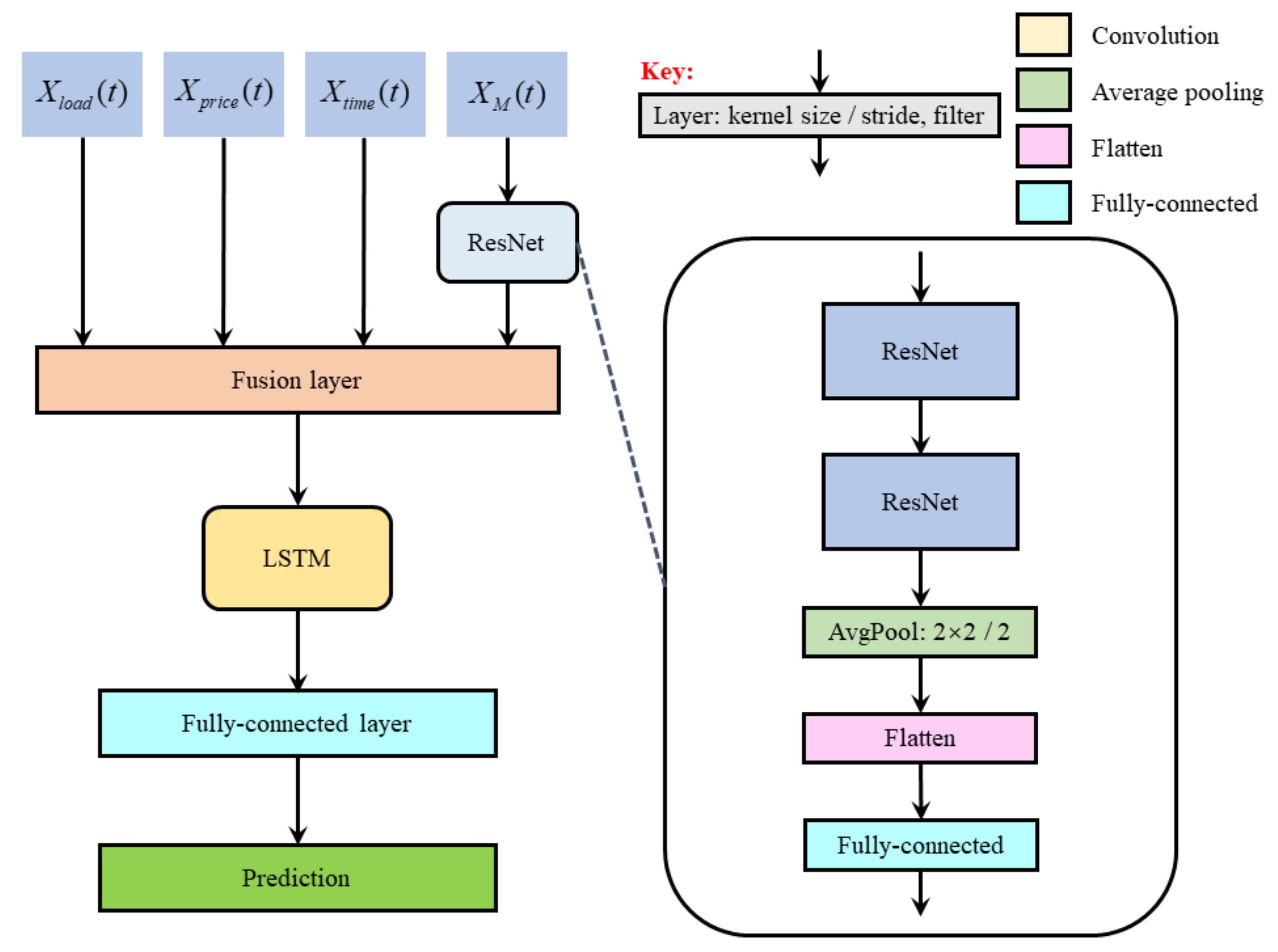
Point forecasting model based on ResNet and LSTM
As illustrated in Figure 4, the point forecasting model based on ResNet and LSTM is also divided into two main subnetworks, the ResNet subnetwork and LSTM subnetwork, which is similar to the above two point forecasting models. The ResNet subnetwork is mainly composed of two ResNet modules, which are used to extract the spatial features of the load EMD component matrix X M ( t ) . The convolutional results of each layer of the ResNet subnetwork are activated by the ReLU activation function.
This is the same as the above two point forecasting models. The input of the LSTM subnetwork is the fusion vector X f ( t ) output by the fusion layer, and X C N N ( t ) changes as an eigenvector extracted by the ResNet subnetwork. The LSTM subnetwork learns the relationship between fusion vector and load, captures the long-term dependence, and realizes the prediction of power load points in the future hour.

3.3. Probabilistic Forecasting Method Based on Quantile Regression Random Forest

The point forecasting models based on VGGNet and LSTM, Inception and LSTM, and ResNet and LSTM were proposed in the previous section. According to the results obtained by the three point forecasting models, quantile regression random forest was used to generate short-term load probabilistic forecasting results at the model end. The frame diagram of the short-term load probabilistic forecasting method based on quantile regression random forest is shown in Figure 5.
For convenience, the definition of some variables is listed in Table 1 where t is the time to be forecast. As shown in Figure 5, the load probabilistic forecasting method based on quantile regression random forest mainly includes four layers, which are the input layer, the feature extraction layer, the forecasting layer, and the output layer.
The feature data required for short-term load probabilistic forecasting are fed to the input layer, including X M ( t ) , X S ( t ) , and V S ( t ) . The feature extraction layer includes four sub-models, which are the three point forecasting sub-models on the basis of VGGNet and LSTM, Inception and LSTM, and ResNet and LSTM, as well as a similar day load selection sub-model. These four sub-models forecast the short-term power load points on the basis of load influencing factors. The forecasting results from these sub-models are the transition forecasting values, which represent the features extracted from the input data. y ˜ 1 ( t ) , y ˜ 2 ( t ) , y ˜ 3 ( t ) , and S d a y ( t ) are the transition point forecasting results obtained from the feature extraction layer. The three point-forecasting models use the subnetworks of VGGNet, Inception, and ResNet to extract the spatial features hidden in the load EMD component matrix. Then, the spatial features are integrated with the information of load, electricity price, and time as the supplementary information and input into the LSTM subnetwork. Next, the LSTM subnetwork captures the long-term dependence in the data and estimates the load value for the next hour.
The similarity daily load selection sub-model uses the similarity defined in Equation (19) to select the 3 days most similar to the day to be predicted from the past 30 days according to the historical loads, prices, and calendar information. In addition, a date 1 year earlier than the predicted date was chosen as another similar date. In the above four similar days, the power load values corresponding to the time to be predicted were extracted as similar daily loads as the prediction output of the sub-model. The similar daily load selection sub-model was used to provide additional effective features for the prediction layer and improve the prediction accuracy of the method.
According to Equation (20) and on the basis of the information of the calendar, the historical power load, and historical electricity prices, the 3 days most similar to the forecast day could be selected from the past 30 days. In addition, the day 1 year earlier than the day to be predicted was also selected as another similar day. In the above four similar days, the power load corresponding to the time to be forecast was extracted as the similar day load and used as the forecasting output of the sub-model. The similar day load selection sub-model was adopted to provide additional effective features for the forecasting layer and improve the forecast accuracy of the method.
The process of the forecasting layer can be divided into two steps. In the first step, the output of feature extraction layer is feature-fused to generate a new feature vector. In the second step, the quantile regression random forest realizes the short-term power load probabilistic forecasting in the form of a quantile based on the new feature vector obtained in the first step.
In the final part of the proposed probabilistic forecasting method, an output layer is constructed to get the short-term power load probabilistic forecasting results.
The training process of can be divided into two stages. In the first stage, the input training data sets are used to train the sub-models in the feature extraction layer. In the second stage, the point forecasting outputs obtained by the four sub-models are used to generate a new dataset, on which the quantile regression random forest of the forecasting layer is trained. In the test process, the test data are input into the feature extraction layer of the four trained sub-models. The final quantile forecasting value is generated by the forecasting layer of quantile regression random forest using the output of the feature extraction layer in the point forecasting model.

4. Numerical Simulations

To verify the validity of the proposed probabilistic forecasting method, a series of simulations were conducted on the basis of the Singapore National Electricity Market electricity load dataset. Hourly data from a total of 35,064 timepoints in 4 years from 2016 to 2019 were selected as training and test datasets. The training samples comprised 75% of the datasets, from 2016 to 2018. The test samples comprised the remaining 25% of the datasets, in 2019. In addition, 0.1, 0.2, 0.3, 0.4, …, 0.9 were selected as the nine quantiles. The number of decision trees in the quantile regression random forest was 200.
The comprehensive evaluation indicator of probabilistic forecasting is introduced in this section. Moreover, the analysis of the probabilistic forecasting results obtained by the proposed method is provided. Lastly, the probabilistic forecasting accuracy of the proposed method is compared with other existing probabilistic forecasting methods.
The probabilistic forecasting model was trained using the efficient Adam optimizer with default parameters as suggested in [23]. All models were built and trained on a desktop PC with a 3.4 GHz Intel i5 processor and 8 GB of memory using the Keras 2.4.3 with Tensorflow 2.3.1 as backend in the Python 3.6 environment. Training the model took approximately 3.2 h.

4.1. Evaluation Indicators

Probabilistic forecasting accuracy is mainly evaluated from the aspects of reliability, sharpness, and resolution. At present, most studies related to load probability forecasting simultaneously consider the above three aspects to comprehensively evaluate the probability forecasting accuracy. Quantity score and Winkler score are the two most commonly used comprehensive indicators.
(1)
Quantity Score
The Global Energy Forecasting Competition 2014 formally introduced probability score into the load forecasting field and put forward quantity score indicator to evaluate the probabilistic forecasting result. The quantity score indicator uses the Pinball loss function to measure the forecast error of the quantile forecast. T is the total number of time points in the test set, K is the total number of the subpoints, and y t is the true load value at t in the test set. The average value of quantity score can be defined as
Avg . QS = 1 T K t = 1 T k = 1 K Pinball ( y ˜ t , q k , y t ) ,
where Pinball ( y ˜ t , q k , y t ) represents the Pinball loss function at quantile q k and time t in the test set. A smaller Avg . QS means a better performance of the probabilistic forecasting method.
(2)
Winkler Score
The Winkler score is a probabilistic forecasting evaluation method proposed by Winkler, which considers both coverage rate and forecast interval width. Let L t and U t denote the lower and upper bounds of the prediction interval, respectively, while δ t is the width of the prediction interval, which is given by
δ t = U t L t .
Then, the Winkler Score at time t can be defined as
WS t = δ t U t y t L t , δ t + 2 ( L t y t ) / α L t > y t , δ t + 2 ( y t U t ) / α U t < y t .
According to the above analysis, when y t is located in the forecast interval and δ t is the smallest, the Winkler score is the minimum. Thus, a smaller Winkler score means a better prediction interval. When Winkler score is used to evaluate the probabilistic forecasting performance, the value at all timepoints should be calculated, and their average is considered as the accuracy of the probabilistic forecasting model using the whole test set. The average value of Winkler score can be defined as
Avg . WS = t = 1 T WS t .
To comprehensively evaluate the probabilistic forecasting performance of the proposed method, the quantile score and Winkler score were both used to evaluate the accuracy of probabilistic forecasting.

4.2. Forecasting Results and Analysis

The probabilistic forecasting method based on the mixed point forecasting model was implemented to obtain the probabilistic forecasting results. The probabilistic forecasting results are analyzed in detail below.
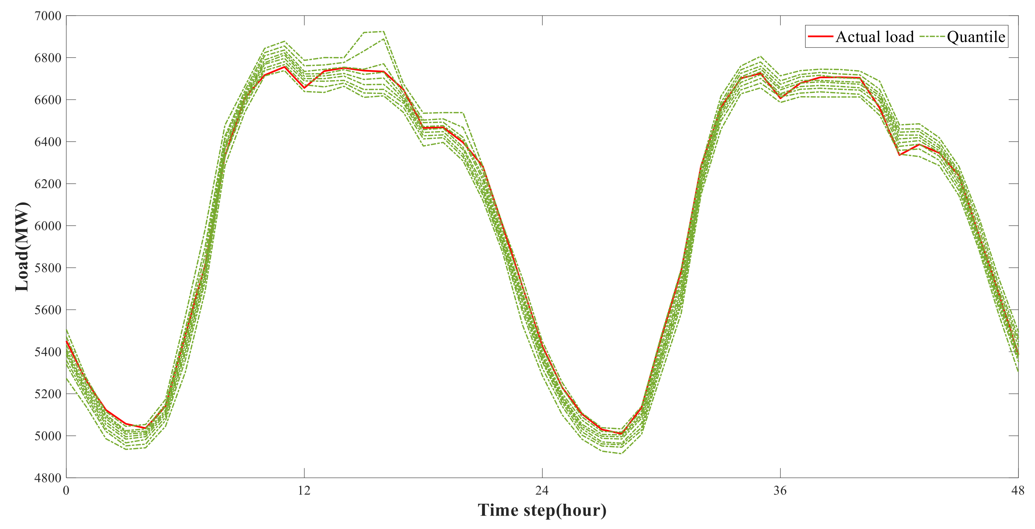
The 48 h load probability prediction results based on the mixed point prediction model are shown in Figure 6 and Figure 7. Figure 6 shows the short-term load probabilistic forecasting results within 48 h on weekdays, and Figure 7 shows the short-term load probabilistic forecasting results within 48 h on weekends. The solid red line represents the actual load, and the dotted green line represents the forecast quantile of load probability from 0.1 to 0.9 with an interval of 0.1. The actual load at each timestep is compared with the forecast quantile. The quantile curve of load probabilistic forecasting can track the overall trend of load change. In most cases, the actual load value stays in the quantile range. Therefore, it is believed that the proposed method has high reliability and accuracy on probabilistic forecasting.
Three existing short-term load probabilistic forecasting methods (quantile gradient enhanced regression tree [24], quantile regression random forest [25], and probabilistic forecasting method based on prediction residual modeling [26]) are introduced to verify the performance improvement of the proposed method. To ensure the fairness and validity of the numerical simulations, all the load probabilistic forecasting methods were tested on the same dataset. The specific information of the three short-term load probabilistic forecasting methods used for comparison is as follows:
(1)
Comparison method 1: quantile gradient enhanced regression tree. This method uses a quantile gradient enhanced regression tree to directly predict short-term load probability. The input features are historical load data and related factors, and the output is the quantile of load.
(2)
Comparison method 2: quantile regression random forest. The quantile regression random forest was briefly introduced in Section 4.1. This method uses quantile regression random forest to directly predict short-term load probability, and the input features are historical load data and related factors.
(3)
Comparison method 3: probabilistic forecasting method based on prediction residual modeling. Firstly, it uses historical load data and related factors to realize a point prediction and obtain the result. Then, the result is used as an additional input feature to describe the conditional distribution of residuals on the point prediction. Finally, the point prediction is combined with the conditional distribution of residuals to obtain the final load probabilistic forecasting result.
The comparison results of the forecast performance based on Avg . QS and Avg . WS with different methods are listed in Table 2. The value of Avg . WS was calculated under the condition α = 60 % . As shown in Table 2, Avg . QS and Avg . WS of the proposed method were significantly smaller than the other three methods on the test set, proving the superiority of the proposed method.
The comparison results of Avg . WS under different confidence levels with the four methods are listed in Table 3. It can be found that, under the same confidence level, Avg . WS of the proposed method was smaller than that of the other three methods. Therefore, compared with the other three methods, the proposed method is more effective in short-term load probabilistic forecasting.
According to the above analysis, compared with comparison methods 1, 2, and 3, the proposed method significantly improved the probabilistic forecasting accuracy, with a smaller prediction interval, higher coverage rate, and higher reliability.
From the above analysis, it can be concluded that, among the three comparison methods, the performance of comparison method 3 was optimal. Therefore, in order to intuitively show the performance improvement of the proposed method, Figure 8 describes the probabilistic forecasting results of the proposed method and comparison method 3 under the confidence level of 80%. The forecast time duration in the figure is from 2 August 2019 to 8 August 2019. The 0.1 and 0.9 quantiles of the forecast results were selected as the upper and lower limits of the forecast interval.
According to the figure analysis, when the confidence level was 80%, the actual load values at most timepoints were within the upper and lower limits of the two methods. Especially in the time periods from peak to trough and trough to peak, the upper and lower limits of the two methods were smaller and more consistent with the actual value. Compared with comparison method 3, the upper and lower bounds of the proposed method were closer to the actual value, and the width of the prediction interval was smaller. In particular, the prediction interval of the proposed method was significantly narrower than that of comparison method 3. During the week from 2 August 2019 to 8 August 2019, the quantile score of comparison method 3 was 15.33 and the quantile score of the proposed method was 15.15. Therefore, in these 2 weeks, the probabilistic forecasting effect of the proposed method was better than that of comparison method 3.
On the basis of the above analysis of short-term load probabilistic forecasting results, the load probabilistic forecasting method based on quantile regression random forest proposed in this paper has high probabilistic forecasting accuracy. Compared with other existing load probabilistic forecasting approaches, the proposed method has a better probabilistic forecasting performance, narrower forecasting interval, higher coverage, and higher reliability, while significantly improving the accuracy of probabilistic forecasting.

5. Conclusions

To solve the problem that the point forecasting model cannot quantify the uncertainty of power load, this paper proposes a short-term load probabilistic forecasting method based on quantile regression random forest. Firstly, three short-term load point forecasting models based on multi-model deep neural networks are established to extract multimodal spatial–temporal features containing more hidden information. Using these three short-term load point forecasting models and the similar day algorithm, the transition point forecasting results can be obtained. According to the forecasting results, the quantile regression random forest method was used to achieve short-term power load probabilistic forecasting. Lastly, taking the Singapore National Electricity Market electricity load dataset as a case study, the comprehensive evolution indicators quantity score and Winkler score were used to measure the short-term probabilistic forecasting accuracy. The numerical simulations showed that, compared to QGERT, QRF, and PFPRM, the proposed method has higher forecasting accuracy and higher reliability.
Although the probabilistic forecasting method proposed in this paper significantly improved the prediction accuracy, due to the limitations of subjective and objective conditions, further research is needed in the following aspects:
(1)
Although LSTM has a strong performance in processing timeseries modeling tasks, its parameters still have some room for optimization. In order to reduce the computation and time consumption of model training and improve computing efficiency, it should be considered to reduce the parameters while keeping the prediction accuracy unchanged.
(2)
In this paper, only historical load, historical load prices, month, week, holiday, and hour information are used to predict the probability of short-term power load. However, in practice, the influencing factors of power load are complicated, and the accurate prediction of short-term power load may not be achieved only by relying on the above features. Therefore, subsequent research needs to consider the influence of other factors on power load such as temperature, humidity, regional economy, and environment, so as to improve the accuracy of short-term load forecasting.
(3)
The data used in this paper only correspond to the Singapore National Electricity Market. In future research, different power load datasets can be selected to train and verify the proposed model and method, as well as optimize it to enhance its generalization ability. In addition, it is also necessary to classify the types of electricity users, such as residential, industrial, and commercial, and construct load probabilistic forecasting models for all types of users according to the differences in the behavior characteristics of each type, so as to provide suggestions for personalized electricity sales services.

Author Contributions

Conceptualization, S.D. and L.P.; methodology, S.D.; software, L.P.; validation, S.D., L.P. and J.Z.; formal analysis, S.D.; data curation, J.Z.; writing—original draft preparation, S.D.; writing—review and editing, J.L. and Z.K. All authors have read and agreed to the published version of the manuscript.

Funding

This research received no external funding.

Data Availability Statement

The data can be obtained from this link: https://www.sgx.com (accessed on: 1 November 2021).

Acknowledgments

This work was supported by the China Southern Power Grid Science and Technology Program 035900KK52200005 (GDKJXM20200741).

Conflicts of Interest

The authors declare no conflict of interest.

References

  1. Kang, C.; Wang, Y.; Xue, Y.; Mu, G.; Liao, R. Big Data Analytics in China’s Electric Power Industry: Modern Information, Communication Technologies, and Millions of Smart Meters. IEEE Power Energy Mag. 2018, 16, 54–65. [Google Scholar] [CrossRef]
  2. Hong, T.; Fan, S. Probabilistic electric load forecasting: A tutorial review. Int. J. Forecast. 2016, 32, 914–938. [Google Scholar] [CrossRef]
  3. Kang, C.; Xia, Q.; Liu, M. Load Forecasting of Power System; China Electric Power Press: Beijing, China, 2007. [Google Scholar]
  4. Li, Z.; Ding, J.; Wu, D.; Wen, F. Integrated extreme learning machine method for power load interval prediction. J. North China Electr. Power Univ. (Nat. Sci. Ed.) 2014, 41, 78–88. [Google Scholar]
  5. Vossen, J.; Feron, B.; Monti, A. Probabilistic forecasting of household electrical load using artificial neural networks. In Proceedings of the 2018 IEEE International Conference on Probabilistic Methods Applied to Power Systems (PMAPS), Boise, Idaho, 23–28 June 2018; pp. 1–6. [Google Scholar]
  6. Zhang, J.; Wang, Y.; Sun, M.; Zhang, N.; Kang, C. Constructing probabilistic load forecast from multiple point forecasts: A bootstrap based approach. In Proceedings of the 2018 IEEE Innovative Smart Grid Technologies-Asia (ISGT Asia), Singapore, 22–25 May 2018; pp. 184–189. [Google Scholar]
  7. Wang, Y.; Gan, D.; Sun, M.; Zhang, N.; Lu, Z.; Kang, C. Probabilistic individual load forecasting using pinball loss guided LSTM. Appl. Energy 2019, 235, 10–20. [Google Scholar]
  8. Chen, K.; Wang, Q.; He, Z.; Hu, J.; He, J. Short-term load forecasting with deep residual networks. IEEE Trans. Smart Grid 2018, 10, 3943–3952. [Google Scholar] [CrossRef] [Green Version]
  9. Zhang, W.; Quan, H.; Srinivasan, D. An improved quantile regression neural network for probabilistic load forecasting. IEEE Trans. Smart Grid 2018, 10, 4425–4434. [Google Scholar] [CrossRef]
  10. Fan, Y.; Fang, F.; Wang, X. Probability forecasting for short-term electricity load based on LSTM. In Proceedings of the 2019 International Conference on Sensing, Diagnostics, Prognostics, and Control (SDPC), Beijing, China, 15–17 August 2019; pp. 516–522. [Google Scholar]
  11. Song, X.; Yang, F.; Wang, D.; Tsui, K.-L. Combined CNN-LSTM network for state-of-charge estimation of lithium-ion batteries. IEEE Access 2019, 7, 88894–88902. [Google Scholar] [CrossRef]
  12. Simonyan, K.; Zisserman, A. Very deep convolutional networks for large-scale image recognition. In Proceedings of the International Conference on Learning Representations, San Diego, CA, USA, 7–9 May 2015. [Google Scholar]
  13. Hochreiter, S.; Schmidhuber, J. Long short-term memory. Neural Comp. 1997, 9, 1735–1780. [Google Scholar] [CrossRef] [PubMed]
  14. He, K.; Zhang, X.; Ren, S.; Sun, J. Deep residual learning for image recognition. In Proceedings of the 2016 IEEE Conference on Computer Vision and Pattern Recognition (CVPR), Las Vegas, NV, USA, 27–30 June 2016; pp. 770–778. [Google Scholar]
  15. Szegedy, C.; Wei, L.; Yangqing, J.; Sermanet, P.; Reed, S.; Anguelov, D.; Erhan, D.; Vanhoucke, V.; Rabinovich, A. Going deeper with convolutions. In Proceedings of the 2015 IEEE Conference on Computer Vision and Pattern Recognition (CVPR), Boston, MA, USA, 7–12 June 2015; pp. 1–9. [Google Scholar]
  16. Liu, B.; Nowotarski, J.; Hong, T.; Weron, R. Probabilistic load forecasting via quantile regression averaging on sister Forecasts. IEEE Trans. Smart Grid 2015, 8, 730–737. [Google Scholar] [CrossRef]
  17. Koenker, R.; Bassett, G., Jr. Regression quantiles. Econom. J. Econom. Soc. 1978, 15, 33–50. [Google Scholar] [CrossRef]
  18. Zhukov, A.; Sidorov, D.N.; Foley, A.M. Random forest based approach for concept drift handling. Commun. Comp. Inf. Sci. 2017. [Google Scholar] [CrossRef] [Green Version]
  19. Breiman, L. Random Forests. Mach. Learn. 2001, 45, 5–32. [Google Scholar] [CrossRef] [Green Version]
  20. Meinshausen, N.; Ridgeway, G. Quantile Regression Forests. J. Mach. Learn. Res. 2006, 7, 984–987. [Google Scholar]
  21. Kurbatsky, V.; Sidorov, D.N.; Spiryaev, V.A.; Tomin, N.V. Forecasting nonstationary time series based on Hilbert—Huang transform and machine learning. Autom. Remote Control 2014, 75, 922–934. [Google Scholar] [CrossRef]
  22. Kurbatskii, V.; Sidorov, D.N.; Spiryaev, V.A.; Tomin, V.N. On the neural network approach for forecasting of nonstationary time series on the basis of the hilbert-huang transform. Autom. Remote Control. 2011, 72, 1405–1414. [Google Scholar] [CrossRef]
  23. Kingma, D.P.; Ba, J. Adam: A method for stochastic optimization. In Proceedings of the 3rd International Conference on Learning Representations (ICLR), SanDiego, MA, USA, 7–9 May 2015. [Google Scholar]
  24. Wang, Y.; Zhang, N.; Tan, Y.; Hong, T.; Kirschen, D.S.; Kang, C. Combining probabilistic load forecasts. IEEE Trans. Smart Grid 2018, 10, 3664–3674. [Google Scholar] [CrossRef] [Green Version]
  25. Zhang, W.; Quan, H.; Srinivasan, D. Parallel and reliable probabilistic load forecasting via quantile regression forest and quantile determination. Energy 2018, 160, 810–819. [Google Scholar] [CrossRef]
  26. Wang, Y.; Chen, Q.; Zhang, N.; Wang, Y. Conditional residual modeling for probabilistic load forecasting. IEEE Trans. Power Syst. 2018, 33, 7327–7330. [Google Scholar] [CrossRef]
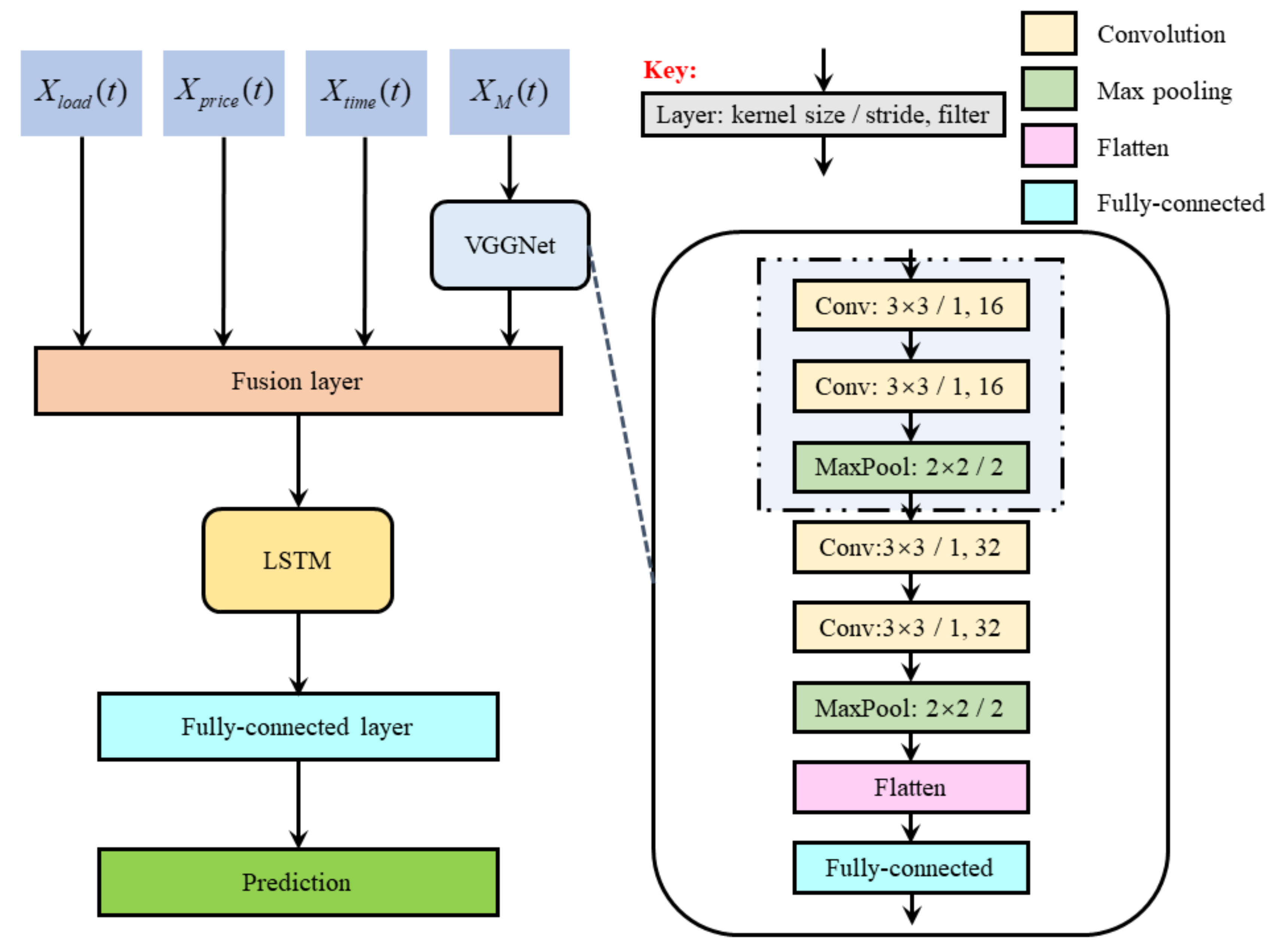
Figure 1. Structure diagram of point forecasting model based on VGGNet and LSTM.
Energies 15 00663 g001
Figure 2. Structure diagram of point forecasting model based on Inception and LSTM.
Energies 15 00663 g002
Figure 3. Inception module internal structure diagram.
Energies 15 00663 g003
Figure 4. Structure diagram of point forecasting model based on ResNet and LSTM.
Energies 15 00663 g004
Figure 5. The frame diagram of the short-term load probabilistic forecasting method based on quantile regression random forest.
Energies 15 00663 g005
Figure 6. Short-term load probabilistic forecasting results within 48 h on weekdays.
Energies 15 00663 g006
Figure 7. Short-term load probabilistic forecasting results within 48 h on weekend.
Energies 15 00663 g007
Figure 8. Short-term load probabilistic forecast for the week from 2 August 2019 to 8 August 2019.
Energies 15 00663 g008
Table 1. Description of the defined variables.
VariableSizeDescription
X S ( t ) (1,379)Input vector containing the load and the electricity price information 168 h before t , and the time information of the hour, week, month, and holiday at t .
V S ( t ) (1,344)Input load influencing factors vector at t .
y ˜ 1 ( t ) (1,1)Output forecasting results obtained by the point forecasting sub-model based on VGGNet and LSTM in the feature extraction layer at t .
y ˜ 2 ( t ) (1,1)Output forecasting results obtained by the point forecasting sub-model based on Inception and LSTM in the feature extraction layer at t .
y ˜ 3 ( t ) (1,1)Output forecasting results obtained by the point forecasting sub-model based on ResNet and LSTM in feature extraction layer at t .
S d a y ( t ) (1,4)Output vector of the forecasting results obtained by the similar day load selection sub-model at t .
Table 2. Comparison results of the short-term load probabilistic forecasting performance with different methods on test sets.
MethodAvg.QSAvg.WS
Comparison method 131.09237.60
Comparison method 230.37233.18
Comparison method 327.26198.72
The proposed method24.44185.80
Table 3. Comparison results of Avg . WS with different methods on test sets under different confidence levels.
Methodα = 20%α = 40%α = 60%α = 80%
Comparison method 1599.85296.87237.60247.76
Comparison method 2601.90282.84233.18269.12
Comparison method 3583.45275.05198.72199.91
The proposed method503.75238.58185.80204.64
Publisher’s Note: MDPI stays neutral with regard to jurisdictional claims in published maps and institutional affiliations.