Feasibility Study on the Influence of Data Partition Strategies on Ensemble Deep Learning: The Case of Forecasting Power Generation in South Korea

Abstract

Ensemble deep learning methods have demonstrated significant improvements in forecasting the solar panel power generation using historical time-series data. Although many studies have used ensemble deep learning methods with various data partitioning strategies, most have only focused on improving the predictive methods by associating several different models or combining hyperparameters and interactions. In this study, we contend that we can enhance the precision of power generation forecasting by identifying a suitable data partition strategy and establishing the ideal number of partitions and subset sizes. Thus, we propose a feasibility study of the influence of data partition strategies on ensemble deep learning. We selected five time-series data partitioning strategies—window, shuffle, pyramid, vertical, and seasonal—that allow us to identify different characteristics and features in the time-series data. We conducted various experiments on two sources of solar panel datasets collected in Seoul and Gyeongju, South Korea. Additionally, LSTM-based bagging ensemble models were applied to combine the advantages of several single LSTM models. The experimental results reveal that the data partition strategies positively influence the forecasting of power generation. Specifically, the results demonstrate that ensemble models with data partition strategies outperform single LSTM models by approximately 4–11% in terms of the coefficient of determination (R²) score.

1. Introduction

Renewable energy refers to the generation of electricity from natural, sustainable resources such as the sun, wind, and water. Solar energy is one of the most popular renewable energy sources. It supplies electric energy to homes or businesses by capturing sunlight. Countries have recently been paying attention to solar energy development because of their advantages: inexhaustible, non-polluting emissions, competitive sources, reducing fossil fuel and natural gas, R² and many others [1]. Even during the COVID-19 pandemic, the solar energy market development did not have a significant impact, excluding some delays due to lockdowns [2]. Like many other countries, South Korea’s government is interested in increasing solar energy usage. More specifically, the government declared the goal of a low-carbon and eco-friendly nation by increasing the renewable energy market to 40% by 2030 from the current 30% [3]. Despite the benefits of solar energy, the provision of electrical energy from solar panels also has some drawbacks. More specifically, there is a high initial investment, ample space required for installing solar panels, and inefficient solar panels [1]. Moreover, solar energy is considered to be intermittent because solar panels produce energy from sunlight. Thus, there are energy storage systems that do not interrupt the power supply. However, persistent bad weather, such as cloudy, rainy, or snowy weather, can result in power outages. Consumers need to monitor weather, electricity production, and consumption to prevent this potential power outage. Energy production forecasting can aid the government’s renewable energy policy as well as help consumers and businesses plan their consumption and develop new products.

Solar panel power generation forecasting is considered a time-series data analysis, which predicts a future outcome based on historical time-stamped data such as the weather. Deep learning methods, particularly long short-term memory (LSTM), have been successfully applied to forecasting time-series data across many domains, including solar panels [4,5,6,7,8,9,10,11,12]. In particular, some studies [4,5,6] have shown the superiority of LSTM models by comparing simple LSTM with other state-of-the-art models, such as back propagation neural networks (BPNN), wavelet neural networks (WNN), support vector machines (SVM), simple recurrent neural networks (RNN), XGBoost, and artificial neural network (ANN). Moreover, incorporating simple LSTM and other deep learning methods such as RNN [7,8], convolutional neural network (CNN) [9,10,11], and autoencoders [12] achieve high performance in forecasting power generation. Even though single LSTM models have achieved significant success in forecasting power generation, single methods may still be weak in overcoming time-series data challenges [13]. More specifically, effectively capturing data characteristics, such as trends, seasonality, and noise robustness, is essential in time-series data analysis.

Ensemble learning-based deep learning methods have shown significant improvements in forecasting the solar panel power generation to overcome these challenges [14,15,16,17,18]. Ensemble learning combines the results from two or more predictive models (i.e., member or base model) to achieve better accuracy than any base model. A common ideology of ensemble learning is that, even if a member is weak in a specific case, the other can be strong. The steps involved in ensemble learning are as follows: (1) base independent models predict an outcome based on various modeling or training data, and (2) ensemble models combine the results of all models to produce a final output. Khan et al. [14] forecasted the solar panel power generation by proposing a stacked ensemble algorithm that combines LSTM and ANN models. The authors reported that the proposed ensemble method demonstrated an improvement in the R² score of 10–12% for a single LSTM and ANN. Pirbazari et al. [15] also predicted solar panel energy generation and household consumption based on an ensemble method combined with several sequence-to-sequence LSTM networks. Experiments on the proposed method showed the potential of the ensemble LSTM to provide more stable and accurate forecasts. Although numerous studies have employed ensemble methods with various data partitioning methods, most have emphasized enhancing the predictive methods by associating many different models or integrating different hyperparameters and interactions. In practice, the performances of ensemble machine learning models are highly dependent on the data partitioning strategy, the number of partitions, and subset sizes. Choosing only a dedicated data partition strategy and subset size may weaken the prediction model for neglected fluctuations. Liang et al. [19] and Wang et al. [20] mentioned the problems of ensemble methods: (1) the number of members significantly affects the accuracy and diversity of ensemble methods, and (2) if the similarity between members is high, the ensemble method may lead to poor performance. Therefore, a feasibility study of data partitioning strategies is essential to effectively reveal the characteristics and features of time-series data and improve the accuracy of power generation forecasting.

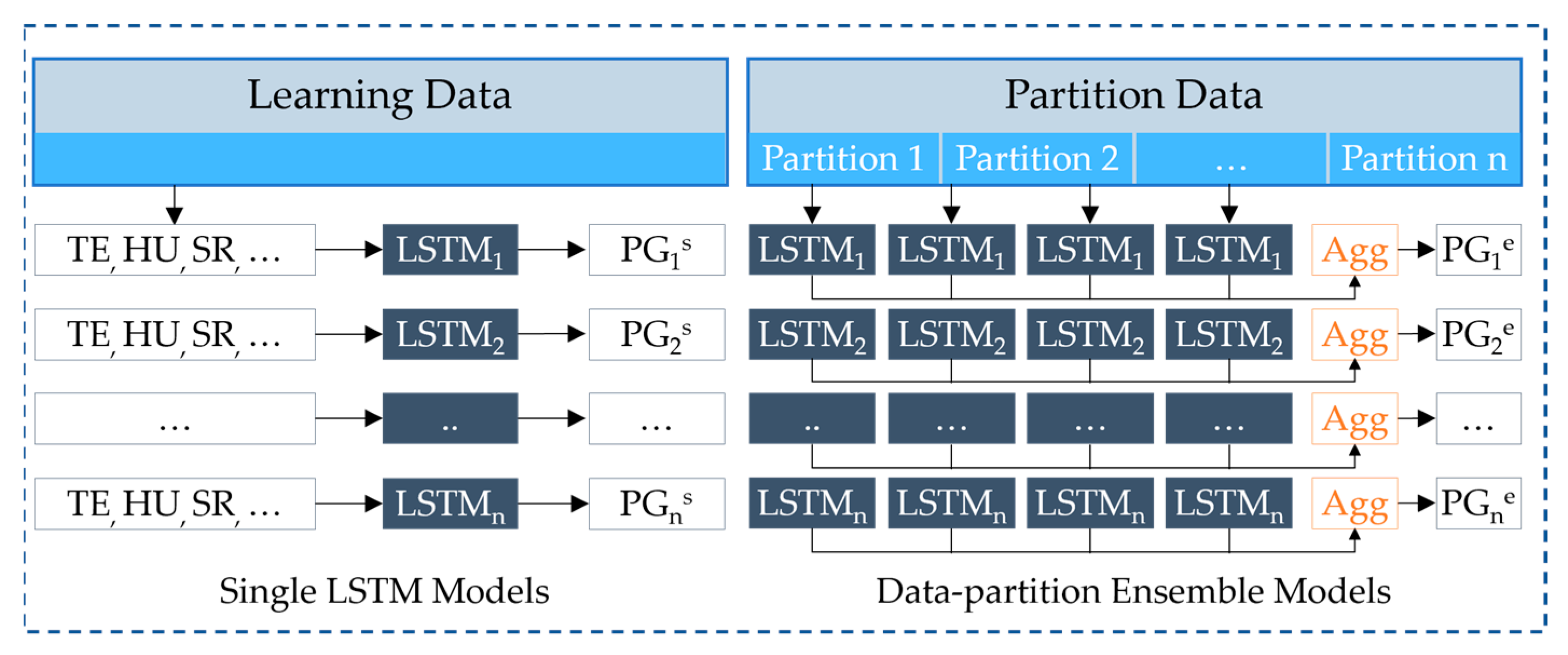
We propose a method for an ensemble deep learning method and data partition strategies to accurately forecast the daily and hourly solar panel power generation. We conducted empirical experiments, in contrast to existing ensemble learning methods, to evaluate the influence of time-series data partition strategies, the number of partitions, and subset sizes. Here, we used an ensemble LSTM model with five time-series data partition strategies: window, shuffle, pyramid, vertical, and seasonal. These data partition strategies enable us to recognize different characteristics and features in time-series data. The main contributions of this study are as follows:

• First, we propose an accurate methodology for forecasting daily and hourly solar panel power generation using an ensemble deep learning model and data partitioning. The method consists of three steps: partitioning time-series data, training models using partitioned subsets, and aggregating the results of each model to obtain the final forecasted power generation.
• Furthermore, we use five simple data partition strategies, namely window, shuffle, pyramid, vertical, and seasonal, to investigate the influence of each strategy on the accuracy of forecasting the solar panel power generation. Data partition strategies are selected to divide the datasets into effective subsets with different characteristics and features in the time-series data. The ensemble model can comprehend multiple characteristics of data by learning from various characteristics. The experiments evaluated the subset sizes and the number of partitions.
• Finally, we evaluated the proposed data partition strategies through extensive experiments using LSTM to forecast the power generation of the solar panels. The experiments examined each data partition using LSTM models with different hyperparameters and checked the influence of different numbers of partitions and subset sizes. We evaluate the experiments on two independent datasets to demonstrate the applicability of the proposed method.

The remainder of this paper is organized as follows: prior studies on the forecasting of solar panel power generation are explained and discussed in Section 2; the materials and methods used in this study are explained in Section 3; the evaluation methods and evaluation results are presented in Section 4; and finally, Section 5 summarizes and concludes this study and discusses future works.

2. Related Work

This section explains the related works that proposed machine learning and deep learning methods to forecasting power generation in renewable energy sources such as wind, hydropower, and solar panels. We explain every study in the following categories: single and ensemble. Additionally, the distinctions between our methodology and that of related studies are discussed.

2.1. Single Methods

Lee et al. [5] predicted the daily solar panel power generation using time-sequential predictive methods: RNN, LSTM, and gated recurrent units (GRU). The monitoring system in Tainan, Taiwan, provided the data that were used in this study. It contains information from three sources, including the Central Weather Bureau of Taiwan, the Environmental Protection Administration of Taiwan, and data from solar power monitoring systems. Experiments in the single inverter showed an accuracy of 89%. Furthermore, the authors used the generative adversarial network (GAN) method to extend the number of inverters to eight. In the experiments, the accuracy (i.e., 93%) of the bidirectional GRU model outperformed other models, such as GRU and LSTM, by approximately 2–17%. Abdel-Nasser and Mahmoud [7] forecasted hourly solar panel power generation using a LSTM-RNN. The experimental results showed that the forecasting error of LSTM was lower than that of other methods, such as multiple linear regression (MLR), bagged regression trees (BRT), and neural networks. The authors noted that the recurrent architecture and memory units of LSTM are efficient for pursuing temporal changes in the solar panel power generation. However, the authors declared the limitations of the study as follows: the effect of outliers was not studied, and environmental features were incorporated.

Deenadayalan and Vaishnavi [21] forecasted the future solar panel power generation and wind turbines using fault identification and remediation. Specifically, the proposed deep learning method consists of parameter adjustment using modified grey wolf optimization (MGWO), fault identification using a CNN-based classifier, power generation forecasts using a regression neural network, and fault remediation using a discriminative gradient. The study dataset was obtained from solar panels and wind turbos in India. The performance analysis of the proposed method showed that the proposed system has a lower error rate than other state-of-art methods. Wang et al. [22] forecasted solar irradiance using a new direct explainable neural network in which it is easy to interpret the prediction result. The proposed network can explain the relationship between the input and the output by extracting the nonlinear mapping features in solar irradiance. The experiments that were conducted using the solar irradiance dataset from Lyon, France, show better prediction performance and explanation. Zsibor’acs et al. [23] studied the difference between day-ahead and intraday solar panel power generation forecasts and the actual generation data in the European Network of Transmission System member states’ operators. The study results show that the intraday forecasts are less skillful than the day-ahead forecasts in all but one of the countries, which highlights the significance of further application-related studies on the intraday horizon. Tu et al. [24] proposed a grey wolf optimization-based general regression neural network for short-term solar power forecasting. The authors claimed that the proposed method provides more accurate predictions with shorter computational times. The performance of their experiments revealed that the proposed method can significantly enhance the prediction accuracy of PV systems.

2.2. Ensemble Methods

Tan et al. [17] explained that it is challenging to develop an accurate and robust model to forecast power demand owing to the intense volatility of industrial power loads. Therefore, they proposed a hybrid ensemble method to forecast ultra-short-term industrial power demand. The ensemble method employs different ensemble strategies such as bagging, random subspace, and boosting. The study evaluated the proposed methods using an open dataset collected from the Australian Energy Market Operator (AEMO), open half-hourly electricity load data from 2013, and a practical dataset from a real-time practical steel plant. The proposed method demonstrated that the ensemble method had greater accuracy and robustness. Wang et al. [18] used a LSTM deep learning model based on the bagging ensemble method to forecast the inflow of hydropower stations. The bagging ensemble method integrates the outputs of member models. There are other ways to integrate the outputs, and this study employs a weighted average, which takes the accuracy of each member model into account. Data from a hydropower station in southern China from 2015 to 2017 was used by the authors. In the experiments, the proposed ensemble method outperformed the other individual models by 0.2% (i.e., deep belief network, random forest regression, GBRT, and LSTM) to 18.7% (i.e., support vector regression). Su et al. [25] proposed a modification to improve the ensemble learning framework for forecasting solar power generation. This study implemented a novel adaptive residual compensation (ARC) algorithm and an evolutionary optimization technique. ARC increases the reliability of conventional models by considering the residuals brought on by prediction mistakes. The authors aimed to forecast the hourly power generation at three solar panel sites. The experimental results proved that the proposed method improves the traditional ensemble methods by approximately 12% in terms of the R² score.

Lotfi et al. [26] presented a novel ensemble method based on kernel density estimation (KDE) to forecast the solar panel power generation. The proposed method forecasts inverter AC power using meteorological variables, such as wind speed, temperature, solar irradiance, precipitation, and humidity. The dataset for one year, from 15 March 2015 to 15 March 2016, was taken from an actual solar panel site located in the vicinity of the city of Coimbra, Portugal. First, the authors calculated the most similar cases from the historical dataset using KDE. The results from all individual models were then ensembled using similar cases in one individual model. The suggested method performed better in the spring, summer, and fall than the irradiance forecast and neural network methods. However, it cannot overcome the limitations of the neural network method in winter. Wen et al. [27] used a hybrid ensemble model to forecast solar panel output intervals. The ensemble model has four individual models: BPNN, radial basis function neural network (RBFNN), extreme learning machine (ELM), and Elman NN. First, the ensemble model forecasts the irradiance, temperature, and wind speed. The authors proposed a ship motion model to predict the power output based on the forecasted features. This study focuses on solar panels deployed on shipboard, in contrast to other solar panel locations. The authors emphasized how the location, date, time zone, and local time, as well as the rolling angle of the ship, affected the solar panel output. The authors designed seven ensemble combination models, and the seventh model, which has members of the BPNN, RBFNN, ELM, and Elman NN, showed the lowest error in root mean squared error (RMSE). Zhang et al. [28] presented an ensemble method to forecast day-ahead power generation in solar panel systems. The dataset of this study comes from free data sources, such as the SolrenView server and the North American Mesoscale Forecast System. The authors combined clustering and blending strategies to improve solar power forecasting accuracy. The proposed forecasting method reduced the normalized RMSE by 13.8–61.21% over the three baseline methods. Kim et al. [29] developed a stacking ensemble SARIMAX-LSTM model for power generation prediction for several solar power plants in various regions of South Korea. The authors used the spatial and temporal characteristics of solar PV generation from satellite images and numerical text data were combined and used. The experimental results revealed that their proposed model outperformed other state-of-art methods, such as SARIMAX, LSTM, Random Forest, and others.

2.3. Discussions

In the field of renewable energy, forecasting power generation benefits from both single and ensemble methods. Even though the single machine learning method has been quite effective in forecasting power generation, the method may not be strong enough to handle time-series data challenges. Therefore, ensemble learning aims to overcome these challenges by combining the results from two or more predictive models to create a more stable and accurate model than single predictive models. Although numerous studies have employed ensemble methods with different data partitioning methods, most of them have focused on enhancing the predictive methods by integrating various models or hyperparameters and interactions. We performed empirical experiments, unlike existing ensemble learning methods, to evaluate the influence of time-series data partition strategies, the number of partitions, and subset sizes.

3. Materials and Methods

3.1. Overview

This study aimed to forecast the solar panel power generation using LSTM and data partitions. Figure 1 illustrates the overall flow of the proposed methodology. This methodology generally consists of the following steps: data fusion, data partitioning, model training, and model evaluation. We concatenated the datasets from different domains based on the DateTime field and applied data preprocessing methods, such as filling missing hours, filling missing values, filtering hours, and scaling. We trained the data-based ensemble LSTM models after prepping the data using various data partitions: window, shuffle, pyramid, vertical, and seasonal. The proposed methodology is evaluated using R², RMSE, and mean absolute error (MAE) which are widely used to measure regression problems. The proposed method is extensively discussed in the subsequent subsections.

3.2. Study Area

This study used datasets from two types of solar panel plants: testbed and actual (Figure 2). The first location (Site A) was a testbed solar panel plant in Seoul, South Korea. The installed capacity of the plant was 30 kW/h. The second location (Site B) was an actual solar panel plant in Gyeongju City, South Korea. The installed capacity of the plant was 1500 kW/h. The datasets of Sites A and B consist of solar panels and weather features, while the dataset of Site A has some additional features, such as power factor and slope. All datasets were provided by Daeyeon C&I [30], a South Korean renewable energy company that has been developing solar power generation and monitoring systems since 1998.

3.3. Data Collection

Table 1. Details of the datasets.

Location	Number of Features	Number of Samples	Date
Site A	12	26,280	1 January 2017~31 December 2019
Site B	8	35,487	1 January 2017~31 December 2020

shows detailed information on the raw datasets before preprocessing. The dataset of Seoul (Site A) consisted of 12 features and 26,280 samples over three years, and the dataset of Gyeongju (Site B) had eight features and 35,487 samples over four years. Both original datasets do not include missing values. The source, name, abbreviation, and description of all the features of the datasets are listed in

Table 2. Feature description of datasets.

Source	Feature	Abbr.	Site A	Site B	Description
Solar panel	Power generation	PG	o	o	The power output of panels (kWh).
	Power factor	PF	o	-	The ratio between the utilized and generated power.
	Slope	SL	o	-	The angle at which the panels are positioned relative to a flat surface.
	Horizontal irradiation	HI	o	-	The total solar radiation incident on a horizontal surface.
	Module temperature	MT	o	-	The temperature of solar panels (°C).
Weather	Temperature	TE	o	o	Outside temperature (°C).
	Humidity	HU	o	o	The concentration of water vapor present in the air (%).
	Cloud	CO	o	o	Amount of cloud.
	Dew point	DP	-	o	Dewpoint (°C).
	Sunshine	SS	o	-	Sunlight reaches the ground without being covered by clouds.
	Solar radiation	SR	o	o	The amount of solar radiation energy on the ground (W/m2).
Derived	Month	MO	o	o	Month of date stamp.
	Hour	HO	o	o	Hour of date stamp.

. These features consist of two primary sources: solar panels and weather. Moreover, we used two more derived features: month and hour. Implementing machine learning or deep learning models on a single dataset might not be convincing due to the likelihood that the chosen dataset could randomly fit the models well. Therefore, we intend to prove the viability of our proposed methodology based on the different locations, features, and characteristics of the two datasets.

3.4. Data Preprocessing

The data preprocessing part generally comprises two sections: exploratory analysis and normalization. Time-series data are collected over time intervals, such as minutes, hours, and days. Time-series data, though, are frequently intermittent in the real world. This issue causes the daily distribution of our datasets to be uneven. Specifically, there are usually data of 24 h a day, but on some days, data of 23 or fewer hours are recorded. In the exploratory analysis, we first filled up these missing hours with NaN values. Next, we filled in the NaN values using the linear interpolation technique. After the datasets were combined, we extracted the relevant information from all the raw data. More specifically, solar panels do not collect power all day, but there are some active hours such as 6 a.m. to 6 p.m. Therefore, data from other hours (i.e., 7 p.m. to 5 a.m.) can affect a prediction model adversely, and this problem is called “bias in the data” in data analysis. Figure 3 shows the power generation of the solar panels by the hour in the Site B dataset. Based on the figure information, data were obtained from 7 a.m. to 5 p.m., and the rest were not used.

Figure 4 shows the correlation between the power generation of the solar panels and the time in the datasets. The data distributions of the datasets were similar, as demonstrated by the figures. The rush hours for solar panels are from 10 a.m. to 3 p.m. Additionally, solar panels produce more power from April to June. The solar panel power generation is low in July and August because they are the rainiest months in South Korea.

Table 3. Five statistical indices of the datasets.

Feature	Site A					Site B
	Count	Mean	Std	Min	Max	Count	Mean	Std	Min	Max
Power generation	12,045	8.89	7.13	0.00	25.76	16,060	525.38	373.94	0.00	1396.85
Power factor	12,045	90.59	22.90	0.00	99.00	-	-	-	-	-
Slope	12,045	353.34	257.74	0.00	942.73	-	-	-	-	-
Horizontal irradiation	12,045	304.26	219.16	0.00	880.52	-	-	-	-	-
Module temperature	12,045	25.09	16.00	−19.79	65.25	-	-	-	-	-
Temperature	12,045	16.66	11.83	−16.81	42.21	16,060	16.11	373.94	−12.90	39.20
Humidity	12,045	51.28	20.46	7.00	100.00	16,060	58.59	23.34	0.00	100.00
Cloud	12,045	5.02	4.00	0.00	10.00	16,060	3.11	3.98	0.00	10.00
Dew point	-	-	-	-	-	16,060	6.81	12.14	−26.90	28.00
Sunshine	12,045	0.60	0.44	0.00	1.00	-	-	-	-	-
Solar radiation	12,045	1.18	0.90	0.00	3.59	16,060	313.00	243.47	0.00	975.00

describes the statistical information of each feature of the datasets after applying the exploratory analysis. The features in the datasets differ significantly from one another. For example, the range of power generation was from 0 to 1400 at Site B, while the range of temperature was from −13 to 39. Therefore, larger differences between the data points of features increase the uncertainty of the prediction models. Consequently, we scaled the datasets using min–max normalization.

3.5. Data Partition

This study proposes a methodology for ensemble LSTM models using several data partition strategies: window, shuffle, pyramid, vertical, and seasonal. Each data partition strategy revealed different characteristics and features in time-series data. These data partition strategies enable us to recognize different features in the time-series data. Moreover, different numbers of partitions and subset sizes are assessed in empirical experiments. The data were first divided by 80% and 20% for learning and testing after preprocessing to process the experiments of the data partition strategies. The learning data was used to extract the training and validation datasets. The evaluation of the prediction models and comparison of the proposed data partition strategies, number of partitions, and subset sizes were performed using the testing data.

3.5.1. Window Data Partition

The window data partition divides the learning data into a given number of partitions by moving a fixed-size window through the learning data samples. The extracted subsets had the same size, and each subset contained similar characteristics because the subsets covers the similar period. This data partition strategy is a straightforward method for reducing the noise in large data samples. Because smaller dataset contains less noise than larger dataset. Algorithm 1 explains the window data partition procedure. The learning data $D$, length of the learning data $N$, length of one partition $n$, and number of data partition $splitN$ are the inputs for the algorithm. The output of the algorithm is a set of partitions $P$. The length of a partition $n$ and the number of partitions $splitN$ are initialized in line 1. In line 2, the algorithm calculates the step size $stepSize$ by dividing the difference between the length of learning data $N$ and the length of one partition $n$ by the difference between the number of partitions $splitN$ and 1. Line 3 selects the partition index from the number of partitions $splitN$. In lines 4–5, the algorithm calculates the start and end indices for data selection. Then, lines 6–7 select the data between the calculated indices and place them into the set of partition $P$. The algorithm is completed in line 8 when the set of partitions is filled by the given number of partitions.

Algorithm 1. Window data partition
Input:	$D$ ← learning data, $N$ ← length of learning data, $n$ ← length of a partition, $splitN$ ← number of partitions
Output:	$P$ ← set of partitions
Procedure:
1	Initialize: $n$, $splitN$
2	Calculate step size: $stepSize=\frac{N-n}{splitN-1}$
3	foreach $i$ in $range\left(0, splitN\right)$ do
4	Calculate start index: $startIndex=i\ast stepSize$
5	Calculate end index: $endIndex=startIndex+n$
6	Select data between the indices: $p=D\left[startIndex:endIndex\right]$
7	Append $p$ into $P$
8	end

3.5.2. Shuffle Data Partition

The shuffle data partition divides the learning data into a given number of fixed-size partitions. The subsets are the same size as the window data partition, and they all contain similar characteristics. It has a similar advantage to the window partition in that it selects a specific part of the training dataset. As opposed to window data partitioning, each partition, in this case, refers to a random portion of the total data. It is also possible that a particular part of the total data does not fit any partition. Algorithm 2 shows the procedure for the shuffle data partition. The inputs and outputs of Algorithm 2 are the same as those of Algorithm 1. In line 1, the length of a partition $n$ and the number of partitions $splitN$ are initialized. Line 2 calculates the highest point that can be selected as a random-start index. If an index exceeds the highest point, we cannot select a partition of $n$ size. In line 3, the repetition of the number of partitions begins. Line 4 obtains a random start index lower than the highest point, and line 5 calculates the end index. Then, lines 6–7 select the data between the calculated indices and put them into the set of partition $P$. The algorithm is completed in line 8 when the set of partitions is filled by the number of partitions.

Algorithm 2. Shuffle data partition
Input:	$D$ ← learning data, $N$ ← length of learning data, $n$ ← length of a partition, $splitN$ ← number of partitions
Output:	$P$ ← set of partitions
Procedure:
1	Initialize $n$, $splitN$,
2	Calculate the limit for start index: $startLimit=N-n$
3	foreach $i$ in $range\left(0, split\_n\right)$ do
4	Get random start index: $startIndex=randomInt\left(0, startLimit\right)$
5	Calculate end index: $endIndex=startIndex+n$
6	Select data between the indices: $p=D\left[startIndex:endIndex\right]$
7	Append $p$ into $P$
8	end

3.5.3. Pyramid Data Partition

The pyramid data partition is a strategy in which the partition size increases from small to large. The first partition was initiated by a fixed-size partition from the center of the data samples. Subsequently, the fixed size was broadened to both sides of the total dataset. Simply put, this data partitioning strategy has the advantage of producing subsets of different sizes, which the ensemble model can combine. Algorithm 3 shows the procedure for the pyramid data partition. The inputs and outputs of Algorithm 3 are identical to those of Algorithms 1 and 2. In line 1, the length of a partition $n$ and the number of partitions $splitN$ are initialized. In lines 2–3, the first start and end indices were calculated. Line 4 calculates the step size, which broadens the start and end indices. In line 5, the repetition of the number of partitions begins. In lines 6 and 9, the algorithm selects the data for a partition. If the start index is equal to or lower than 0, the total learning data is selected as a partition (Line 7). In contrast, a partition is selected between the start and end indices. In line 10, the algorithm places the selected data into a set of partitions. In lines 10–11, the $startIndex$ is updated by subtracting the step size from the start index, and the $endIndex$ is updated by adding the step size to the end index. The algorithm is completed in line 13 when the set of partitions is filled by the number of partitions.

Algorithm 3. Pyramid data partition
Input:	$D$ ← learning data, $N$ ← length of learning data, $n$ ← length of a partition, $splitN$ ← number of partitions
Output:	$P$ ← set of partitions
Procedure:
1	Initialize $n$, $splitN$,
2	Calculate the first start index: $startIndex=N-n$
3	Calculate the first end index: $endIndex=startIndex+n$
4	Calculate the step size: $stepSize=\frac{startIndex}{splitN-1}$
5	foreach $i$ in $range\left(0, split\_n\right)$ do
6	$\hspace{1em}\hspace{1em}if startIndex\le 0$then
7	Get all dataset $p=D$
8	$\hspace{1em}\hspace{1em}else$then
9	Get data between the indices: $p=D\left[startIndex:endIndex\right]$
10	Append $p$ into $P$
11	Update start index: $startIndex=startIndex-stepSize$
12	Update end index: $endIndex=endIndex+stepSize$
13	end

3.5.4. Vertical Data Partition

The vertical data partition strategy splits the learning dataset vertically rather than horizontally, in contrast to other data partition strategies. It splits datasets by selecting a subset of relevant variables and reduces dimensionality. It is inspired by variable selection methods in machine learning. A set of features is first created by manually. Specifically, all the features of the datasets were divided into several subsets. In Site A, the feature sets consist of “Slope, Power Factor, Horizontal Irradiation, PV Temperature, Temperature,” “Power Factor, Horizontal Irradiation, PV Temperature, Temperature, Humidity,” “Horizontal Irradiation, PV Temperature, Temperature, Humidity, Sunshine,” “PV Temperature, Temperature, Humidity, Sunshine, Solar Radiation,” and “Temperature, Humidity, Sunshine, Solar Radiation, Cloud.” At Site B, the feature sets consisted of “Temperature, Humidity,” “Humidity, Dew Point,” “Dew Point, Solar Radiation,” and “Solar Radiation, Cloud.” Additionally, “Month” and “Hour” features are added to all subsets. Algorithm 4 shows the procedure for the vertical data partition. The inputs for the algorithm are the learning data $D$, and feature sets $S$. The output of the algorithm is a set of partitions $P$. In line 1, the feature set $S$ is initialized. Line 2 selects a feature set from all feature sets. In lines 3–4, the algorithm creates partitions based on the selected features. The algorithm is completed in line 5.

Algorithm 4. Vertical data partition
Input:	$D$ ← learning data, $S$ ← feature sets
Output:	$P$ ← set of partitions
Procedure:
1	Initialize $S$
2	foreach $s$ in $S$ do
3	Select data related to the set $s$: $p=D\left[s\right]$
4	Append $p$ into $P$
5	end

3.5.5. Seasonal Data Partition

Seasonal data partitioning is a two-level data partition strategy. It can be used to catch the seasonal features of the datasets. Algorithm 5 presents the procedure for seasonal data partitioning. First, the datasets were divided into subsets by time-logical splitters, such as monthly or hourly. Monthly, we split the datasets based on seasons, such as winter (December, January, and February), spring (March, April, and May), summer (June, July, and August), and autumn (September, October, and November). We split the datasets based on three hours ranges: morning (7-10), noon (11-14), and evening (15-17). Each subset was then subjected to a window partition strategy. The datasets were split based on seasonal factors, which created subsets with similar characteristics and improved the accuracy and stability of the model. The reason for this is that the predictive model can always learn from the same time ranges, such as the winter, summer, morning, or evening.

Algorithm 5. Seasonal data partition
Input:	$D$ ← learning data, $N$ ← length of learning data, $S$ ← set of seasonal data $n$ ← length of a partition, $splitN$ ← number of partitions
Output:	$P$ ← set of partitions
Procedure:
1	Initialize: $S$ by splitting D by seasonal (i.e., Monthly or Hourly)
2	foreach s in S do
3	Based on the subset initialize: $n$, $splitN$, $N$
4	Calculate step size: $stepSize=\frac{N-n}{splitN-1}$
5	foreach $i$ in $range\left(0, splitN\right)$ do
6	Calculate start index: $startIndex=i*stepSize$
7	Calculate end index: $endIndex=startIndex+n$
8	Select data between the indices: $p=D\left[startIndex:endIndex\right]$
9	Append $p$ into $P$
10	end
11	end

3.6. Training of LSTM Models

In this study, our principal predictive model was LSTM, an expendable type of RNN that overcomes the problem of long-term dependencies. Learning important parts and forgetting less important parts in sequence data makes LSTM prevalent in time-series data forecasting [31,32,33,34]. Figure 5 shows the structures of the LSTM models. It consists of two concepts: single and data partition ensemble LSTM models. We first used the entire learning data for different hyperparameters to train $n$ single LSTM models. Single models were specifically trained using the same data but different hyperparameters. After that, we used data partition strategies to create a dataset. The set contained $n$ training and validation data combinations. Subsequently, the data partition ensemble LSTM methods aggregate the outputs of the same single LSTM models.

4. Results

4.1. Dataset

This study conducted two types of experiments: a single LSTM and a data partition ensemble LSTM. The number of training and validation data for each experiment was slightly different. However, we used the same test data for all experiments to check the effectiveness of our methodology.

Table 4. Summary of datasets used in experiments.

LSTM		Site A			Site B
		Train	Validation	Test	Train	Validation	Test
Single		7231	2407	2407	9640	3210	3210
Data-based ensemble	Window	7200	1800	2407	8000	2000	3210
	Shuffle	7200	1800	2407	8000	2000	3210
	Pyramid	8000~9638	1600~1928	2407	8000~12850	1600~2570	3210
	Vertical	7231	2407	2407	9640	3210	3210
	Seasonal	2991~3618	318~1000	2407	1990~2969	43~1000	3210

summarizes the datasets used in the experiments. The last 20% of the total data were test data at each site. The remaining data were split by training and validation based on the methodology. We selected the same number of test data from the training data in the single LSTM models as the validation data. In total, 20% of the training data were used as validation data in the data partition ensemble methods.

4.2. Evaluation Metrics

We evaluated the experiments in this study by using three standard measures of regression problems. Specifically, R², RMSE, and MAE are provided in Equations (1)–(3). Here, $i$ and $n$ are the index of the sample and number of samples, respectively. Moreover, $y$, $\widehat{y}$, and $\overline{y}$ are the actual values, forecasted values, and mean of the actual values, respectively. R² measures the accuracy of a regression model with a value between 0 and 1. A value closer to 1 indicates that the model fits the data better. We multiplied R² by 100 to represent the accuracy as a percentage. The residuals or prediction errors are assumed to be the cause of the discrepancy between the actual and forecasted values. The standard deviation of the residuals is known as RMSE. MAE is a measure of errors between actual and forecasted values without considering their direction. A lower RMSE and MAE suggest that the actual and forecasted values are closer.

$$R^2=\left(1-\frac{{{\displaystyle \sum }}_{i=1}^n{\left(y_i-\widehat{y_i}\right)}^2}{{{\displaystyle \sum }}_{i=1}^n{\left(y_i-\overline{y}\right)}^2}\right)\times 100$$

(1)

$$RMSE=\sqrt{\frac{{{\displaystyle \sum }}_{i=1}^n{\left(y_i-\widehat{y_i}\right)}^2}{n}}$$

(2)

$$MAE=\frac{{{\displaystyle \sum }}_{i=1}^n\left|y_i-\widehat{y_i}\right|}{n}$$

(3)

4.3. Experimental Results

Table 5. Hyperparameter settings of the LSTM models.

LSTM	Optimizer	Learning Rate	Epochs	Batch Size	Patience	Units
Single	ADAM	0.001	1000	32	30	60,70,80,90,100
Ensemble	ADAM	0.001	1000	32	30	60,70,80,90,100

lists the hyperparameters of the proposed methods, such as single LSTM, model-based ensemble LSTM, and data-based ensemble LSTM. Our model consists of two layers, such as LSTM and fully connected, which returns final prediction value. We found that the ADAM optimizer with a learning rate of 0.001 was the optimal hyperparameter during several training sessions with different optimizers and learning rates. The number of epochs indicates how frequently the model trained the entire training dataset. In model training, setting the right epoch is crucial because low epochs might cause underfitting issues. High epochs, on the other hand, can result in overfitting issues and prolonged training time. The EarlyStopping function generally stops training if the accuracy cannot be increased during the number (i.e., patience) of epochs. Therefore, we set epochs to 1000 and early stopping with patience to 30. We trained the individual LSTM models with 60, 70, 80, 90, and 100 units. Subsequently, these single LSTM models were compared with the ensemble LSTM models.

4.3.1. Hourly Forecasting of Site A

Table 6. Experimental results of hourly forecasting of Site A.

Methods	LSTM60			LSTM70			LSTM80			LSTM90			LSTM100
	R2	RMSE	MAE	R2	RMSE	MAE	R2	RMSE	MAE	R2	RMSE	MAE	R2	RMSE	MAE
No partition	94.44	1.56	0.80	94.94	1.49	0.60	94.07	1.61	0.77	93.58	1.68	0.94	93.93	1.63	0.82
Window	97.95	0.95	0.47	97.98	0.96	0.50	97.97	0.94	0.49	97.89	0.96	0.45	98.18	0.89	0.41
Shuffle	97.94	0.95	0.45	97.74	1.00	0.51	97.99	0.94	0.44	97.93	0.95	0.45	98.19	0.89	0.38
Pyramid	96.52	1.24	0.83	96.68	1.17	0.76	96.96	1.16	0.74	96.94	1.16	0.64	97.49	1.05	0.62
Vertical	95.30	1.44	0.74	96.56	1.23	0.68	96.17	1.30	0.68	95.98	1.33	0.68	96.23	1.29	0.66
Seasonal	98.31	0.86	0.33	98.23	0.88	0.34	98.05	0.93	0.33	98.22	0.89	0.32	98.22	0.89	0.34

exhibits experimental results for forecasting power generation hourly in Site A. The table shows that all data partition strategies improve the accuracies of single LSTM models. More specifically, the seasonal data split technique consistently delivers the best results. The fundamental explanation is that we only train and evaluate the ensemble model during a particular season, such as the summer. Here, we discover that the ensemble model of seasonal partition with unit 60 is the best model to forecast the amount of energy per hour. This model outperforms other single LSTM models by around 3.4–4.7%.

Figure 6 shows the hourly forecasted power generation results for Site A. In the figure, we selected the results of the last 32 h of the test datasets, where the blue line represents the actual values, and the dashed lines represent the best cases in each data partition strategy. It is difficult to distinguish between the actual and forecasted values if the entire test dataset is selected. The figure illustrates that the results of data partitioning schemes more closely match actual observations than the results of a single model.

4.3.2. Daily Forecasting of Site A

Table 7. Experimental results of daily forecasting of Site A.

Methods	LSTM60			LSTM70			LSTM80			LSTM90			LSTM100
	R2	RMSE	MAE	R2	RMSE	MAE	R2	RMSE	MAE	R2	RMSE	MAE	R2	RMSE	MAE
No partition	90.09	12.84	10.10	93.98	10.00	7.15	92.98	10.80	7.99	87.84	14.22	10.86	86.81	14.81	11.73
Window	95.92	8.30	5.38	95.25	8.96	5.92	94.12	9.97	6.33	95.78	8.45	5.26	94.93	9.25	5.99
Shuffle	95.52	8.70	5.52	95.67	8.55	5.17	94.26	9.85	6.27	96.39	7.81	4.94	96.23	7.98	4.81
Pyramid	93.91	10.14	7.21	92.30	11.40	8.79	90.49	12.68	9.22	94.00	10.07	7.22	93.61	10.39	7.30
Vertical	88.59	13.88	10.16	92.75	11.07	6.93	94.14	9.95	5.79	93.22	10.70	6.81	92.53	11.23	6.77
Seasonal	98.00	5.77	2.88	98.00	5.78	2.91	97.49	6.47	3.16	97.89	5.93	2.92	97.73	6.15	2.95

displays the experimental findings for the daily power generation forecasting in Site A. The table demonstrates that, with the exception of specific vertical data partition strategy cases, all data partition strategies improve the accuracy of single LSTM models. Like the window data partition, the seasonal data partition strategy performs best in all cases. Here, we find that the best model to forecast the amount of energy per hour is the ensemble model of seasonal partition with unit 60. This model outperforms other single LSTM models by around 4–11.2%.

Figure 7 shows the hourly forecasted power generation results for Site A. In the figure, we selected the results of the last month of the test datasets, where the blue line represents the actual values, and the dashed lines represent the best cases in each data partition strategy. From the figure, we can see that the results of the data partition strategies follow the actual observations better than those of the single model.

4.3.3. Hourly Forecasting of Site B

Table 8. Experimental results of hourly forecasting of Site B.

Methods	LSTM60			LSTM70			LSTM80			LSTM90			LSTM100
	R2	RMSE	MAE	R2	RMSE	MAE	R2	RMSE	MAE	R2	RMSE	MAE	R2	RMSE	MAE
No partition	85.15	140.91	104.32	84.43	144.28	104.83	84.66	143.21	105.55	84.53	143.84	106.33	85.18	140.77	102.98
Window	86.85	132.61	94.09	86.87	132.50	95.01	87.11	131.28	94.05	87.21	130.77	92.85	87.18	130.92	93.09
Shuffle	87.11	131.26	91.97	87.31	130.28	91.38	87.31	130.28	91.93	87.36	130.00	91.26	87.55	129.03	90.76
Pyramid	86.97	131.98	93.33	87.32	130.20	91.80	86.92	132.26	96.40	87.44	129.62	91.23	86.93	132.22	94.12
Vertical	85.78	137.88	100.20	85.58	138.86	99.50	86.13	136.16	98.23	85.95	137.08	98.10	86.44	134.63	95.96
Seasonal	88.64	125.17	89.47	88.60	125.36	89.93	88.42	126.36	91.47	89.05	122.88	88.30	88.69	124.86	88.85

shows experimental results for forecasting power generation hourly in Site B. The table demonstrates how all data partition strategies increase the accuracies of single LSTM models. More specifically, the seasonal data partition strategy performs best in all cases. Here, we find that the best model to forecast the amount of energy per hour is the ensemble model of seasonal partition with unit 90. This model outperforms other single LSTM models by around 3.9–4.6%. Figure 8 exhibits the results for hourly forecasting power generation in Site B. We selected the test dataset results from the most recent 21 h to exhibit in the figure. The figure demonstrates that the results of data partition strategies more closely match actual observations than the results of a single model.

4.3.4. Daily Forecasting of Site B

Table 9. Experimental results of daily forecasting of Site B.

Method	LSTM60			LSTM70			LSTM80			LSTM90			LSTM100
	R2	RMSE	MAE	R2	RMSE	MAE	R2	RMSE	MAE	R2	RMSE	MAE	R2	RMSE	MAE
No partition	83.68	928.77	677.82	83.84	924.18	664.43	85.76	867.54	624.75	85.07	888.24	633.74	85.69	869.49	635.16
Window	87.19	822.94	613.09	86.47	845.68	640.72	86.34	849.73	639.83	87.36	817.29	603.58	87.90	799.55	581.59
Shuffle	86.67	839.39	615.75	86.68	838.86	625.65	86.06	858.30	639.80	87.10	825.70	612.01	87.08	826.28	591.23
Pyramid	87.22	821.65	596.28	87.11	825.51	616.56	87.34	817.85	605.42	87.12	824.90	605.30	87.14	824.25	593.65
Vertical	83.90	922.40	693.93	84.26	912.06	693.72	82.81	953.26	725.32	82.17	970.77	735.92	83.20	942.34	725.87
Seasonal	89.33	738.98	560.45	87.94	785.68	592.60	89.04	749.03	564.35	88.50	767.23	568.71	88.72	759.93	574.78

shows experimental results for daily power generation forecasting in Site B. The table demonstrates that, with the exception of specific vertical data partition strategy scenarios, all data partition strategies increase the accuracy of single LSTM models. Like the window data partition, the seasonal data partition strategy performs best in all cases. Here, we find that the best model to forecast the amount of energy per hour is the ensemble model of seasonal partition with unit 60. This model outperforms other single LSTM models by around 3.6–5.7%.

Figure 9 shows the results of forecasting power generation daily at Site B. In the figure, we selected the results of the last month of the test datasets, where the blue line represents the actual values, and the dashed lines represent the best cases in each data partition strategy. From the figure, we can see that the results of the data partition strategies follow the actual observations better than those of the single model.

4.3.5. Comparison of Seasonal Partition

We used two types of seasonal splitters, monthly and hourly, in the seasonal partition. We evaluated these two cases and used the better ones in the following experiments. Figure 10 shows the monthly and hourly split experimental results by the R² score. Here, using the months outperforms the hourly results, except at Site A. The results were similar at Site A. Therefore, we used the monthly split in subsequent experiments.

4.3.6. Partition Length and Subset Size

This experiment evaluated the relationship between the forecasting performance and different numbers of partitions and subset sizes. To this end, we ran three data partition strategies (window, shuffle, and pyramid) with five combinations of the number of partitions (5, 8, and 10) and subsite sizes (60%, 70%, and 80% of training data).

Table 10. Experimental results of comparing the partition length and subset size.

Site	Method	5_60%			5_70%			5_80%			8_80%			10_80%
		R2	RMSE	MAE	R2	RMSE	MAE	R2	RMSE	MAE	R2	RMSE	MAE	R2	RMSE	MAE
A/Hourly	Window	97.69	1.01	0.46	98.16	0.90	0.41	97.82	0.98	0.53	97.81	0.98	0.49	97.92	0.96	0.49
A/Hourly	Shuffle	95.97	1.33	0.67	97.22	1.10	0.61	97.86	0.97	0.50	97.91	0.95	0.47	98.02	0.93	0.44
A/Hourly	Pyramid	98.13	0.91	0.41	98.05	0.93	0.45	98.05	0.92	0.45	97.98	0.94	0.48	98.03	0.93	0.45
A/Daily	Window	95.49	8.73	5.22	95.71	8.51	5.11	93.65	10.36	6.67	90.86	12.43	8.37	92.16	11.59	8.21
A/Daily	Shuffle	93.78	10.25	5.41	94.96	9.23	5.57	96.68	7.49	4.72	96.66	7.50	4.65	96.85	7.30	4.44
A/Daily	Pyramid	96.59	7.59	4.66	95.86	8.37	5.06	96.31	7.90	4.72	96.37	7.84	4.70	95.99	8.23	4.99
B/Hourly	Window	87.41	129.75	91.54	87.44	129.61	91.81	85.97	137.00	95.11	87.44	129.60	91.44	87.63	128.63	89.72
B/Hourly	Shuffle	86.60	133.85	94.93	86.75	133.09	95.28	86.96	132.02	94.19	87.21	130.79	92.12	87.20	130.81	92.87
B/Hourly	Pyramid	87.40	129.78	90.67	87.48	129.39	90.60	87.56	128.98	90.34	87.39	129.83	90.24	87.39	129.85	90.94
B/Daily	Window	87.25	820.82	595.05	87.31	818.91	600.47	86.25	850.59	620.11	87.93	798.74	615.01	87.66	852.59	625.11
B/Daily	Shuffle	86.84	833.96	613.85	87.14	824.47	604.91	87.09	826.10	609.20	87.25	820.96	604.14	87.03	827.99	614.89
B/Daily	Pyramid	87.61	809.27	592.22	87.68	806.86	583.62	87.81	802.59	588.31	87.87	800.62	595.06	87.75	804.36	596.45

presents the detailed results of these experiments. The results specify the number of partitions, subset sizes, and optimal data partition strategy for each dataset. Specifically, the best number of partitions and subset sizes were determined as follows:

• Site A, hourly forecasting: window partition strategy with five partitions and subset size of 70%.
• Site A, daily forecasting: shuffle partition strategy with ten partitions and a subset size of 80%.
• Site B, hourly forecasting: window partition strategy with ten partitions and 80% subset size.
• Site B, daily forecasting: window partition strategy with eight partitions and subset size of 80%.

5. Discussion and Conclusions

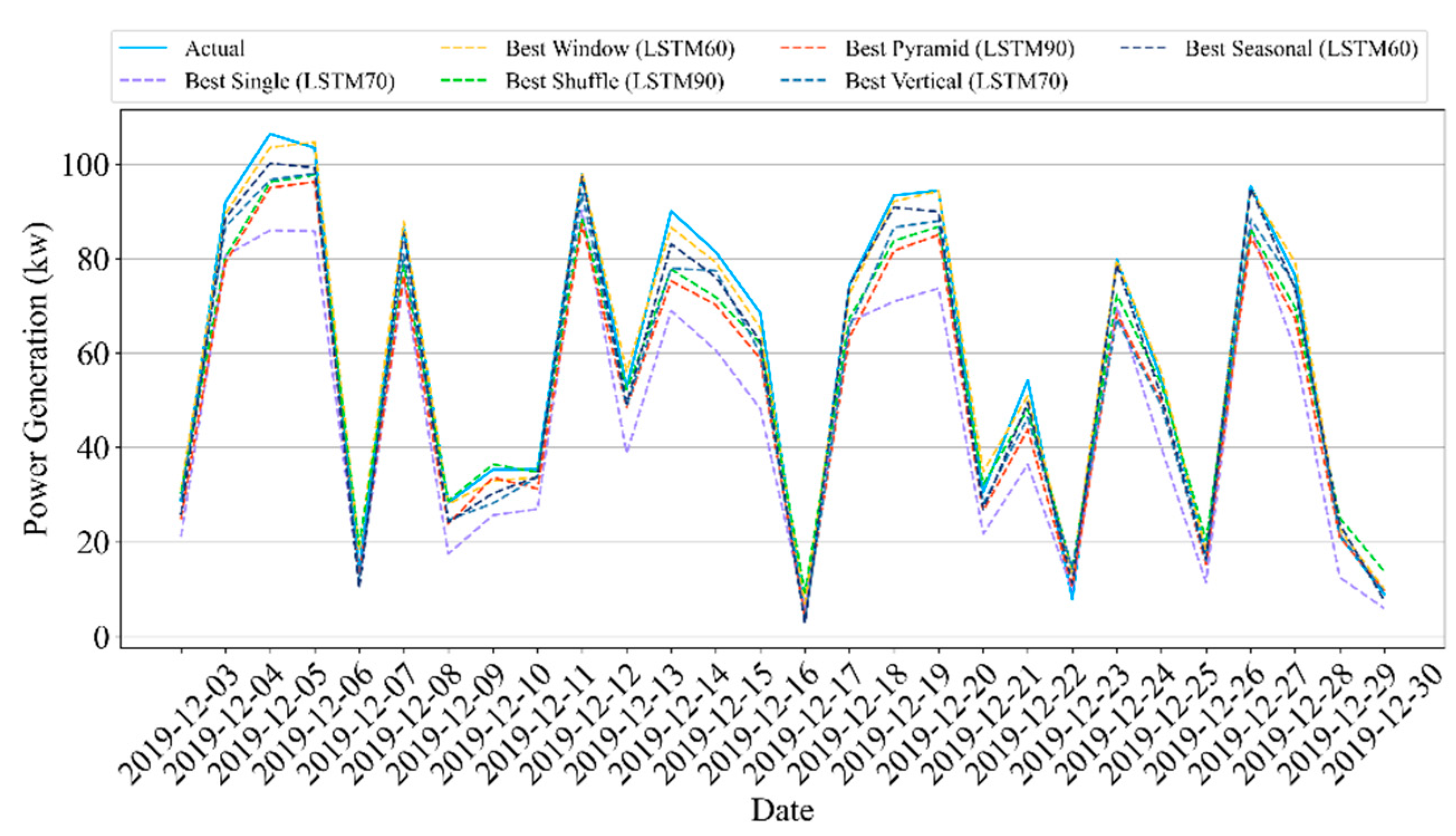
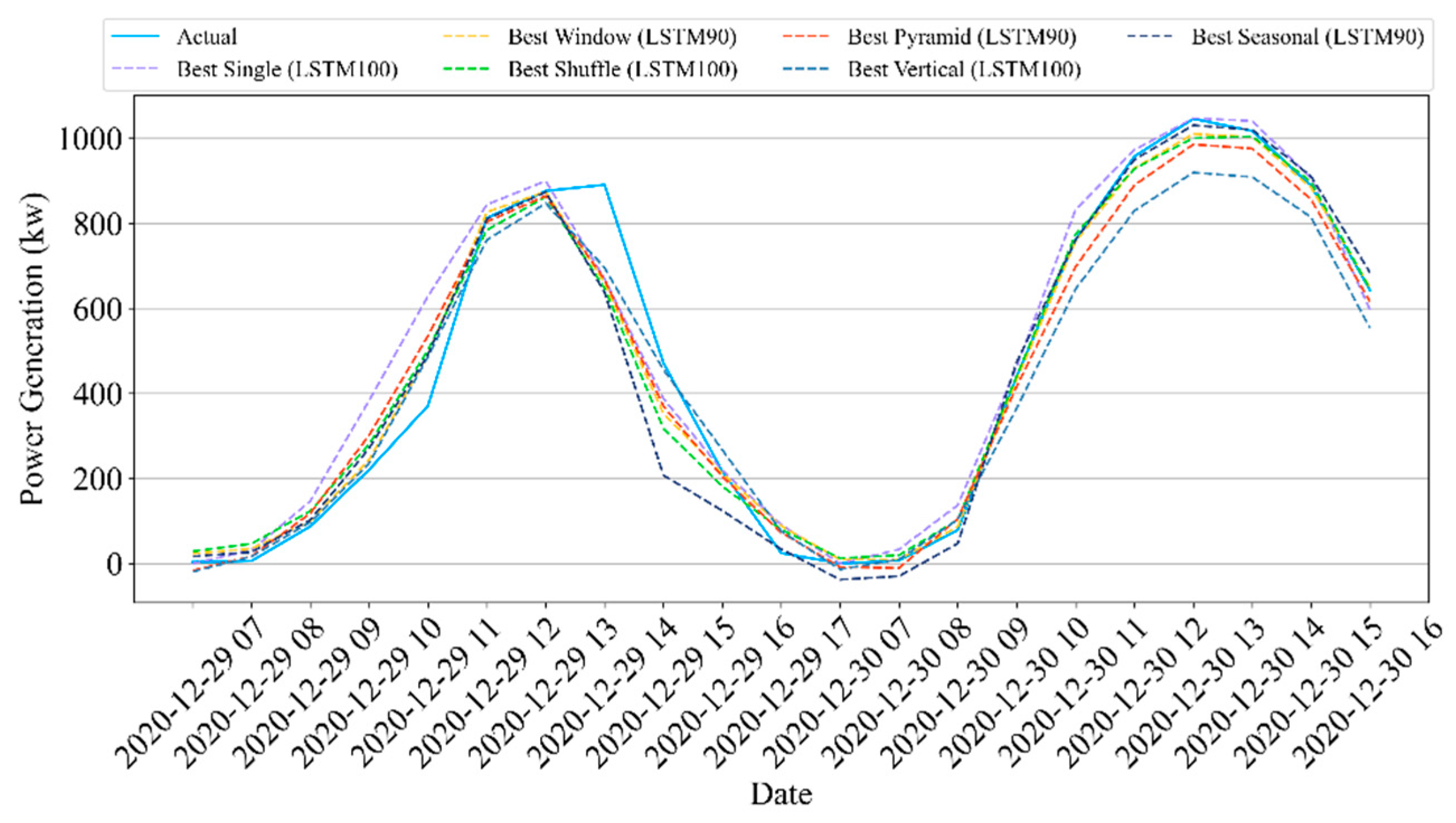
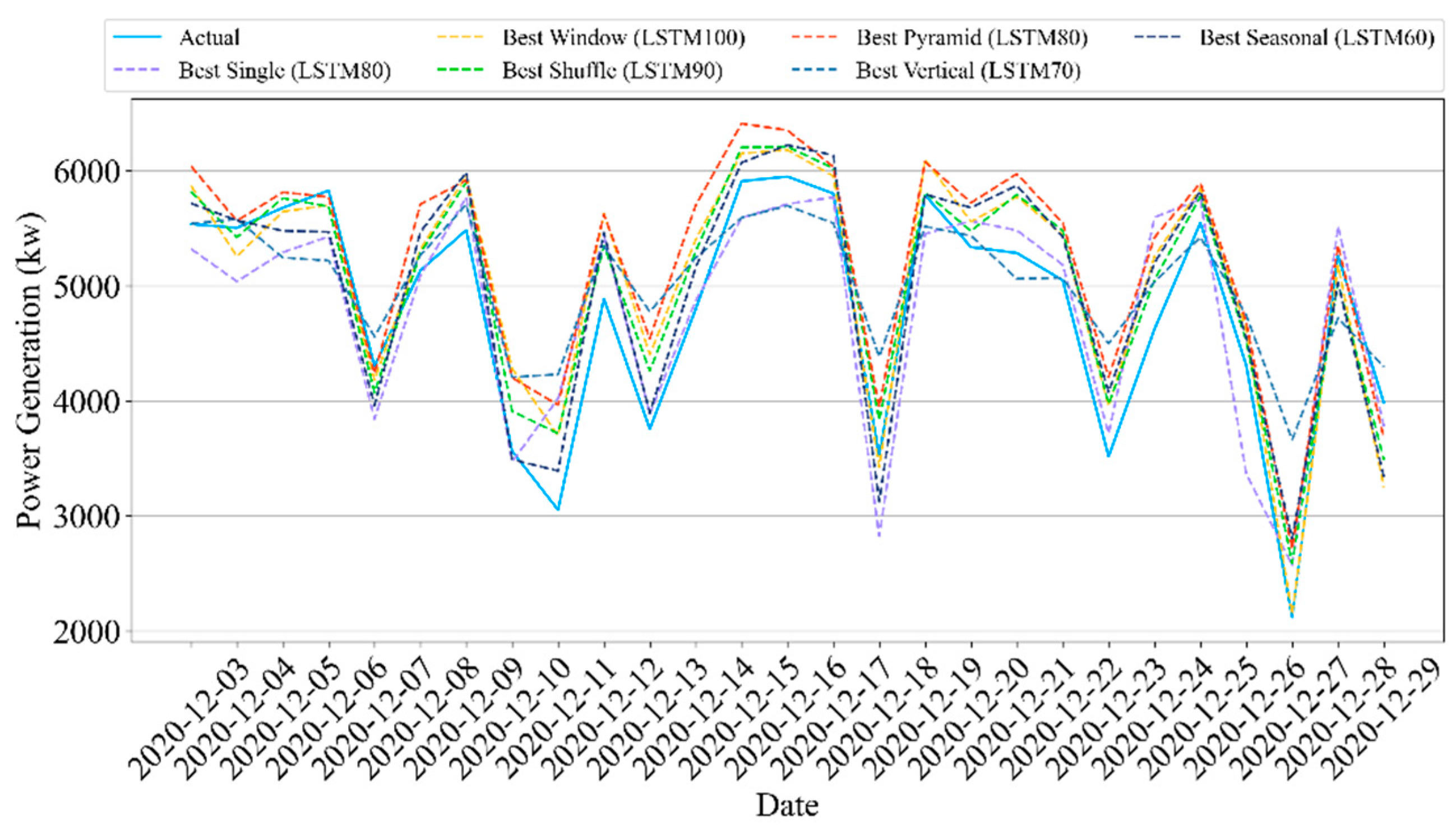
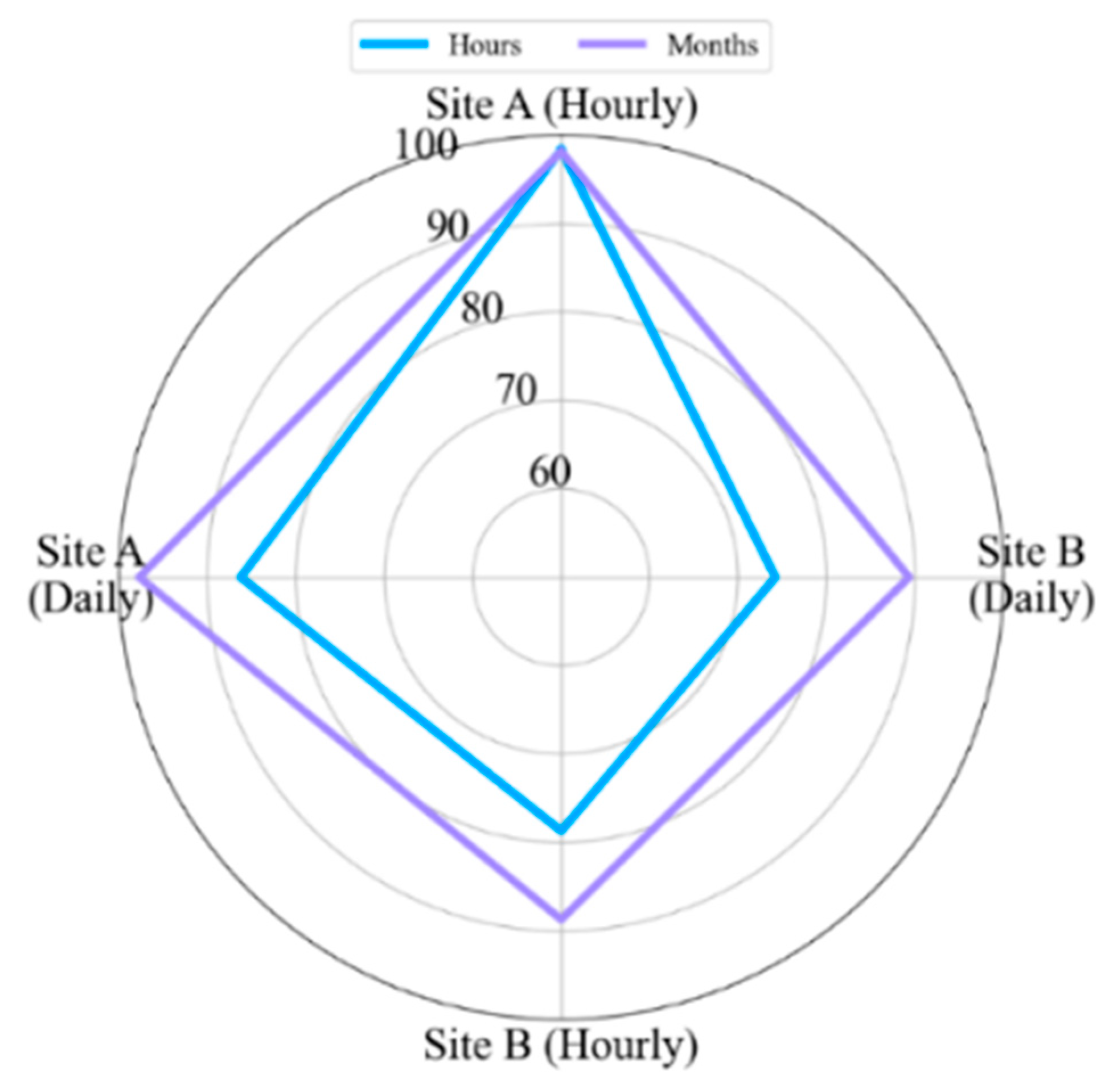
This study presented a methodology that forecasts the hourly and daily solar panel power generation using ensemble LSTM models and five data partition strategies: window, shuffle, pyramid, vertical, and seasonal. We intended to explore the influences of different time-series data partition strategies, the number of partitions, and subset sizes on the performance of the ensemble LSTM model. The extensive experimental results compared the concepts of LSTM methods using testbed (i.e., Site A) and real-world (i.e., Site B) solar panel data.

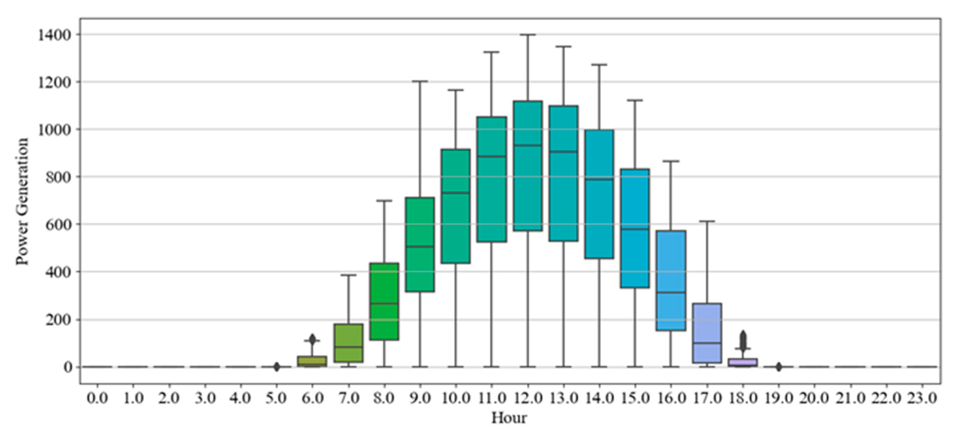
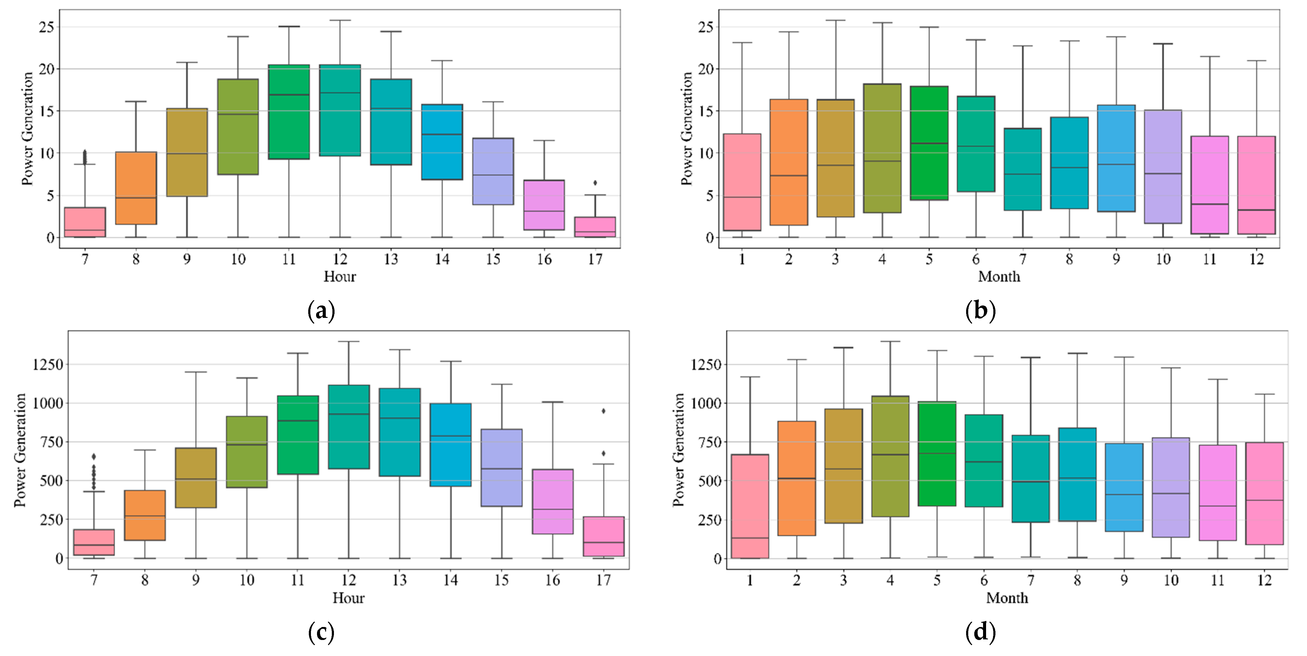
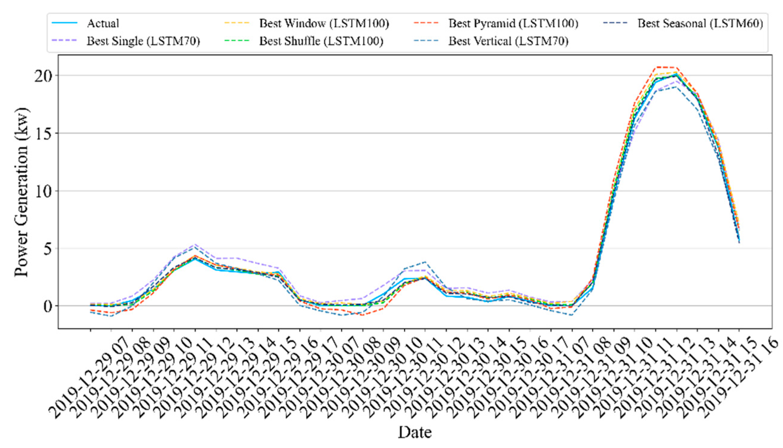
We first implemented five single LSTM models with different units using identical training and test data. The single models had an R² scores of 93.6–94.9% and 84.4–85.2% for Sites A and B, respectively, in hourly forecasting. For daily forecasting, Sites A and B had R2 scores of 86.8–94% and 83.7–85.8%, respectively. Second, the data partition ensemble LSTM model outperformed all single LSTM models in the experimental cases. More specifically, the results were as follows: Sites A and B had R² scores of 95.3–98.3% and 85.6–89%, respectively, in hourly forecasting and 90.5–98% and 82.2–89.3%, respectively, in daily forecasting. Particularly, the two-level seasonal data partition strategy showed good performance improvements. Solar panel power generation depends highly on seasons. If we compare winter and summer, winter days are shorter than summer days. Because of shorter days, the sun angle on solar panels changes rapidly in winter. On the contrary, the sun goes higher and stays longer in summer. Additionally, the winter months have more stormy and cloudy weather. Based on these reasons, the collected solar panel power generation data have different features for each season. Training prediction model for each season helps us to reduce high variance and bias. Additionally, we investigated the relationship between performance and the number of partitions as well as the size of subsets. The results indicated that adding more training data did not improve performance.

The experiments proved that the proposed data partition ensemble LSTM methods forecast the hourly and daily solar panel power generation more accurately and reliably. Integrating solar energy monitoring with forecasting models increases the performance of solar panel systems and provides advantages to all participants in the sector, such as government, businesses, and consumers. Using this system, solar energy consumers can reconcile their electricity usage and avoid unexpected power outages and unnecessary costs. Additionally, businesses can give customers additional options and products. Furthermore, the data generated from the models can be used to improve and develop plans. Governments have been promoting renewable energy and have set time-bound goals. Efficient electricity consumption by consumers will help to make government goals more realistic.

This study demonstrated that data partitioning has positive influences on forecasting the solar panel power generation, even though we used simple strategies. However, unlike methods such as clustering, these strategies cannot account for the relationship between the data. Therefore, we plan to study more logical strategies for data partitioning in future study. Consequently, each part of the data contains appropriate data points and helps improve the forecasting performance.

References

1. Guangul, F.M.; Chala, G.T. Solar energy as renewable energy source: SWOT analysis. In Proceedings of the 4th MEC International Conference on Big Data and Smart City (ICBDSC), Muscat, Oman, 15–16 January 2019. [Google Scholar]
2. International Energy Agency. Snapshot of Global PV Markets 2021; Report IEA-PVPS T1-39; International Energy Agency: Paris, France, 2021. [Google Scholar]
3. Korea Energy Agency. National Survey Report of PV Power Applications in Korea; Korea Energy Agency: Yongin-si, Korea, 2019. [Google Scholar]
4. Gao, M.; Li, J.; Hong, F.; Long, D. Day-ahead power forecasting in a large-scale photovoltaic plant based on weather classification using LSTM. Energy 2019, 187, 115838. [Google Scholar] [CrossRef]
5. Lee, C.-H.; Yang, H.-C.; Ye, G.-B. Predicting the performance of solar power generation using deep learning methods. Appl. Sci. 2021, 11, 6887. [Google Scholar] [CrossRef]
6. Zheng, J.; Zhang, H.; Dai, Y.; Wang, B.; Zheng, T.; Liao, Q.; Liang, Y.; Zhang, F.; Song, X. Time series prediction for output of multi-region solar power plants. Appl. Energy 2020, 257, 114001. [Google Scholar] [CrossRef]
7. Abdel-Nasser, M.; Mahmoud, K. Accurate photovoltaic power forecasting models using deep LSTM-RNN. Neural Comput. Appl. 2019, 31, 2727–2740. [Google Scholar] [CrossRef]
8. Wang, F.; Xuan, Z.; Zhen, Z.; Li, K.; Wang, T.; Shi, M. A day-ahead PV power forecasting method based on LSTM-RNN model and time correlation modification under partial daily pattern prediction framework. Energy Convers. Manag. 2020, 212, 112766. [Google Scholar] [CrossRef]
9. Wang, K.; Qi, X.; Liu, H. A comparison of day-ahead photovoltaic power forecasting models based on deep learning neural network. Appl. Energy 2019, 251, 113315. [Google Scholar] [CrossRef]
10. Wang, K.; Qi, X.; Liu, H. Photovoltaic power forecasting based LSTM-Convolutional Network. Energy 2019, 189, 116225. [Google Scholar] [CrossRef]
11. Ghimire, S.; Deo, R.C.; Raj, N.; Mi, J. Deep solar radiation forecasting with convolutional neural network and long short-term memory network algorithms. Appl. Energy 2019, 253, 113541. [Google Scholar] [CrossRef]
12. Gensler, A.; Henze, J.; Sick, B.; Raabe, N. Deep Learning for solar power forecasting—An approach using AutoEncoder and LSTM Neural Networks. In Proceedings of the 2016 IEEE International Conference on Systems, Man, and Cybernetics (SMC), Budapest, Hungary, 9–12 October 2016. [Google Scholar]
13. Dong, X.; Yu, Z.; Cao, W.; Shi, Y.; Ma, Q. A survey on ensemble learning. Front. Comput. Sci. 2020, 14, 241–258. [Google Scholar] [CrossRef]
14. Khan, W.; Walker, S.; Zeiler, W. Improved solar photovoltaic energy generation forecast using deep learning-based ensemble stacking approach. Energy 2022, 240, 122812. [Google Scholar] [CrossRef]
15. Pirbazari, A.M.; Sharma, E.; Chakravorty, A.; Elmenreich, W.; Rong, C. An ensemble approach for multi-step ahead energy forecasting of household communities. IEEE Access. 2021, 9, 36218–36240. [Google Scholar] [CrossRef]
16. Singla, P.; Duhan, M.; Saroha, S. An ensemble method to forecast 24-h ahead solar irradiance using wavelet decomposition and BiLSTM deep learning network. Earth Sci. Inform. 2022, 15, 291–306. [Google Scholar] [CrossRef] [PubMed]
17. Tan, M.; Yuan, S.; Li, S.; Su, Y.; Li, H.; He, F.H. Ultra-short-term industrial power demand forecasting using LSTM based hybrid ensemble learning. IEEE Trans. Power Syst. 2020, 35, 2937–2948. [Google Scholar] [CrossRef]
18. Wang, L.; Peng, H.; Tan, M.; Pan, R. A multistep prediction of hydropower station inflow based on bagging-LSTM model. Discret. Dyn. Nat. Soc. 2021, 2021, 1031442. [Google Scholar] [CrossRef]
19. Liang, J.; Wei, P.; Qu, B.; Yu, K.; Yue, C.; Hu, Y.; Ge, S. Ensemble learning based on multimodal multiobjective optimization. In Bio-inspired Computing: Theories and Applications, Proceedings of the International Conference on Bio-Inspired Computing: Theories and Applications, Zhengzhou, China, 22–25 November 2019; Pan, L., Liang, J., Qu, B., Eds.; Springer: Singapore, 2020; Volume 1159, p. 1159. [Google Scholar]
20. Wang, X.; Han, T. Transformer fault diagnosis based on stacking ensemble learning. IEEJ Trans. Electr. Electron. Eng. 2020, 15, 1734–1739. [Google Scholar] [CrossRef]
21. Deenadayalan, V.; Vaishnavi, P. Improvised deep learning techniques for the reliability analysis and future power generation forecast by fault identification and remediation. J. Ambient. Intell. Humaniz. Comput. 2021, 1–9. [Google Scholar] [CrossRef]
22. Wang, H.; Cai, R.; Zhou, B.; Aziz, S.; Qin, B.; Voropai, N.; Gan, L.; Barakhtenko, E. Solar irradiance forecasting based on direct explainable neural network. Energy Convers. Manag. 2020, 226, 113487. [Google Scholar] [CrossRef]
23. Zsibor´acs, H.; Pint´er, G.; Vincze, A.; Baranyai, H.; Mayer, M.J. The reliability of photovoltaic power generation scheduling in seventeen European countries. Energy Convers. Manag. 2022, 260, 115641. [Google Scholar] [CrossRef]
24. Tu, C.-S.; Tsai, W.-C.; Hong, C.-M.; Lin, W.-M. Short-Term Solar Power Forecasting via General Regression Neural Network with GreyWolf Optimization. Energies 2022, 15, 6624. [Google Scholar] [CrossRef]
25. Su, H.-Y.; Liu, T.-Y.; Hong, H.-H. Adaptive residual compensation ensemble models for improving solar energy generation forecasting. IEEE Trans. Sustain. Energy 2020, 11, 1103–1105. [Google Scholar] [CrossRef]
26. Lotfi, M.; Javadi, M.; Osório, G.J.; Monteiro, C.; Catalão, J.P.S. A novel ensemble algorithm for solar power forecasting based on kernel density estimation. Energies 2020, 13, 216. [Google Scholar] [CrossRef] [Green Version]
27. Wen, S.; Zhang, C.; Lan, H.; Xu, Y.; Tang, Y.; Huang, Y. A hybrid ensemble model for interval prediction of solar power output in ship onboard power systems. IEEE Trans. Sustain. Energy 2021, 12, 14–24. [Google Scholar] [CrossRef]
28. Zhang, X.; Li, Y.; Lu, S.; Hamann, H.F.; Hodge, B.-M.; Lehman, B. A solar time based analog ensemble method for regional solar power forecasting. IEEE Trans. Sustain. Energy 2019, 10, 268–279. [Google Scholar] [CrossRef]
29. Kim, B.; Suh, D.; Otto, M.-O.; Huh, J.-S. A Novel Hybrid Spatio-Temporal Forecasting of Multisite Solar Photovoltaic Generation. Remote Sens. 2021, 13, 2605. [Google Scholar] [CrossRef]
30. Daeyeon C&I Co., LTD. Available online: http://dycni.com/ (accessed on 26 March 2022).
31. Sagheer, A.; Kotb, M. Time series forecasting of petroleum production using deep LSTM recurrent networks. Neurocomputing 2019, 323, 203–213. [Google Scholar] [CrossRef]
32. Pheng, T.; Chuluunsaikhan, T.; Ryu, G.-A.; Kim, S.-H.; Nasridinov, A.; Yoo, K.-H. Prediction of process quality performance using statistical analysis and long short-term memory. Appl. Sci. 2022, 12, 735. [Google Scholar] [CrossRef]
33. Ai, S.; Chakravorty, A.; Rong, C. Evolutionary Ensemble LSTM based Household Peak Demand Prediction. In Proceedings of the International Conference on Artificial Intelligence in Information and Communication (ICAIIC), Okinawa, Japan, 11–13 February 2019. [Google Scholar]
34. Zhao, F.; Zeng, G.Q.; Lu, K.D. EnLSTM-WPEO: Short-term traffic flow prediction by ensemble LSTM, NNCT weight integration, and population extremal optimization. IEEE Trans. Veh. Technol. 2019, 69, 101–113. [Google Scholar] [CrossRef]
Figure 1. Overall flow of the proposed methodology. Here, the abbreviations of the features are described in Table 2; R2: Coefficient of Determination; RMSE: Root Mean Squared Error; MAE: Mean Absolute Error.
Energies 15 07482 g001
Figure 2. Locations of the study areas.
Energies 15 07482 g002
Figure 3. Solar panel power generation by hour Site B.
Energies 15 07482 g003
Figure 4. Power generation of (a) hourly in Site A, (b) monthly in Site A, (c) hourly in Site B, and (d) monthly in Site B.
Energies 15 07482 g004
Figure 5. Training structure of the LSTM models.
Energies 15 07482 g005
Figure 6. Results of hourly forecasting of Site A.
Energies 15 07482 g006
Figure 7. Results of daily forecasting of Site A.
Energies 15 07482 g007
Figure 8. Results of hourly forecasting of Site B.
Energies 15 07482 g008
Figure 9. Results of daily forecasting of Site B.
Energies 15 07482 g009
Figure 10. Comparison of seasonal partition.
Energies 15 07482 g010