
A Method for the Identification of Critical Interstop Sections in Terms of Introducing Electric Buses in Public Transport


Abstract
:1. Introduction
- -
- Which bus routes may be affected by only minor delays, making them suitable for electric buses?
- -
- Which sections of the road and street network cause the most delays in public transport?
2. Related Literature
3. Research Method
3.1. The Main Assumptions of the Method
- -
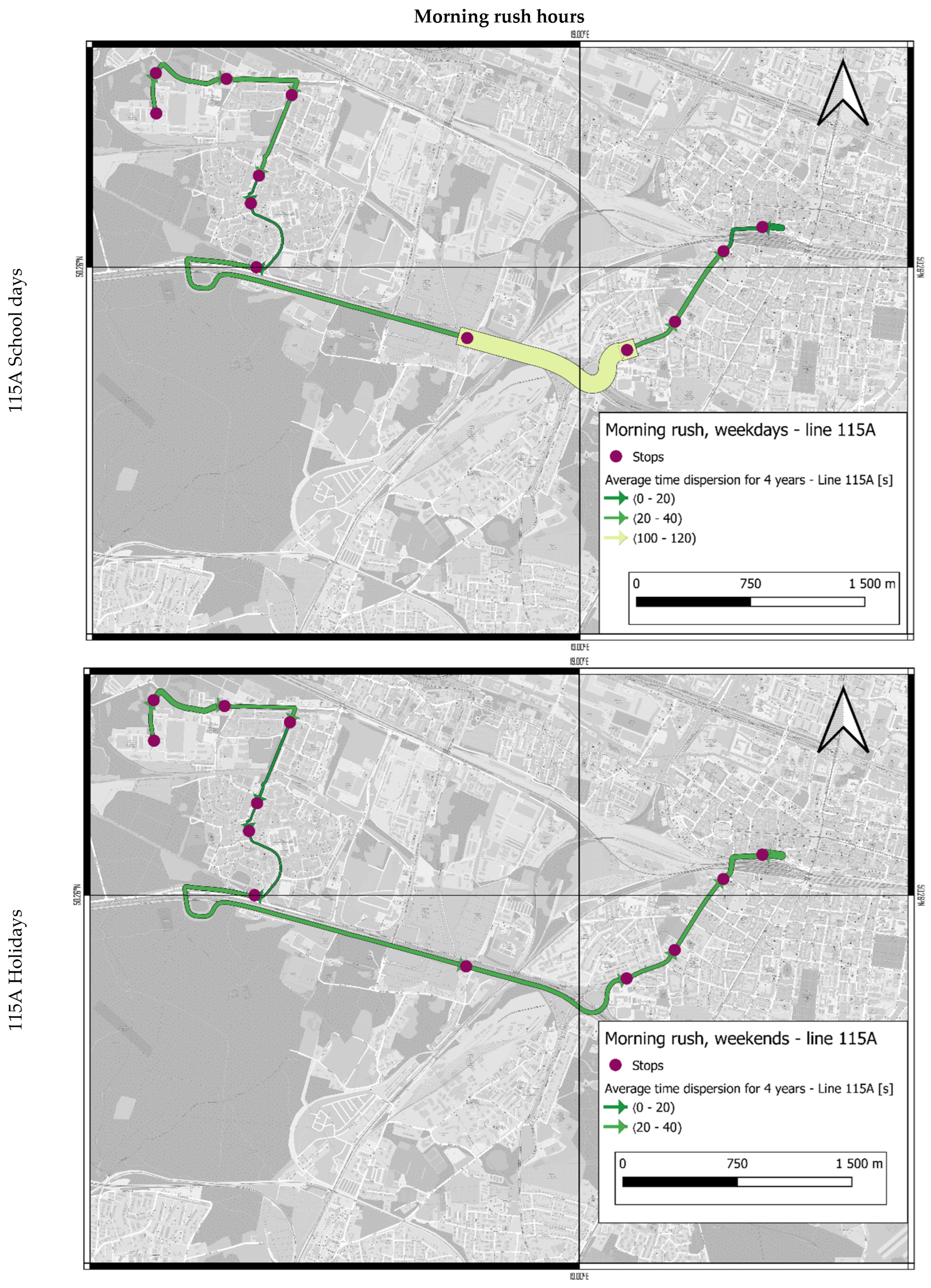
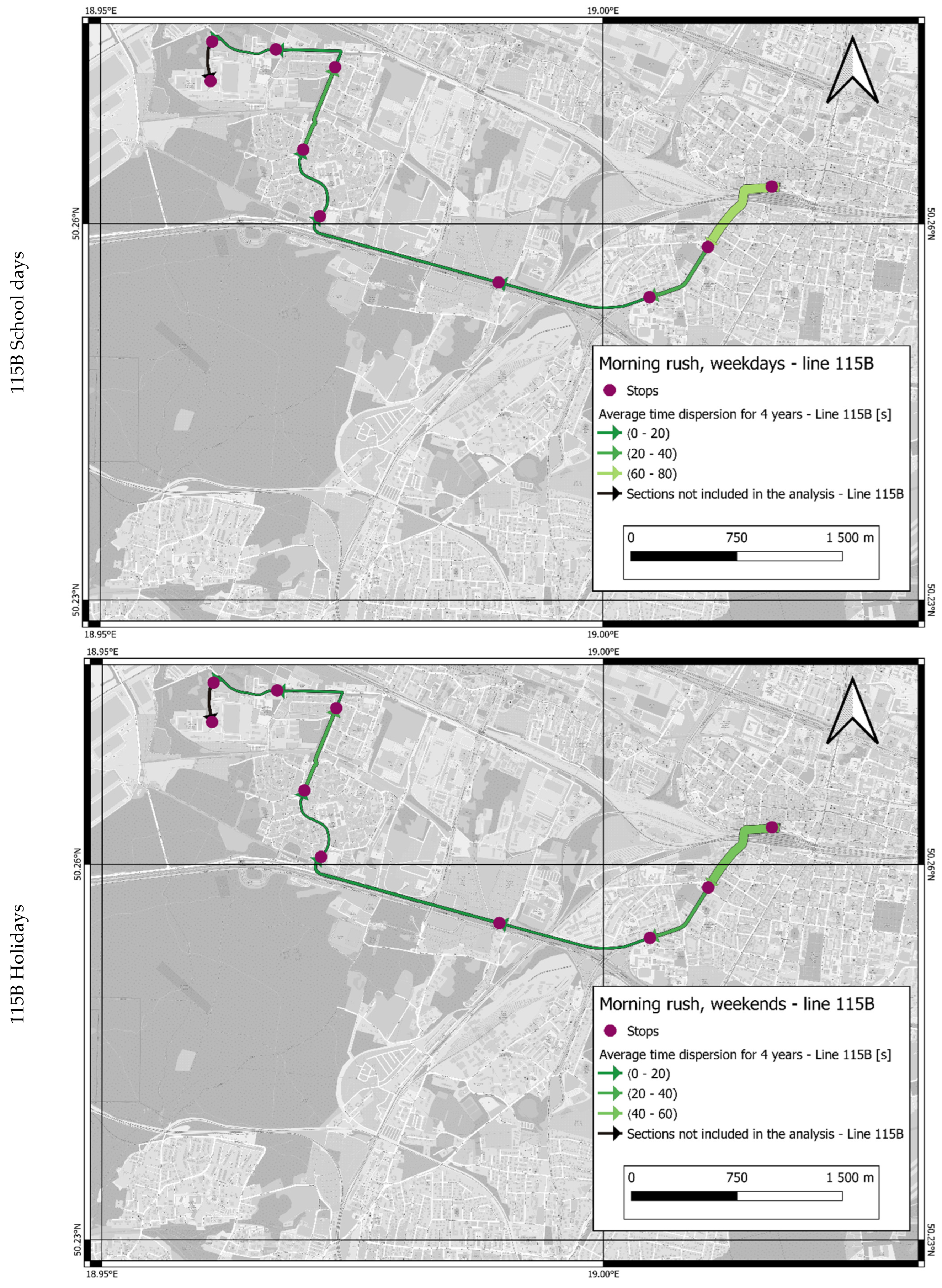
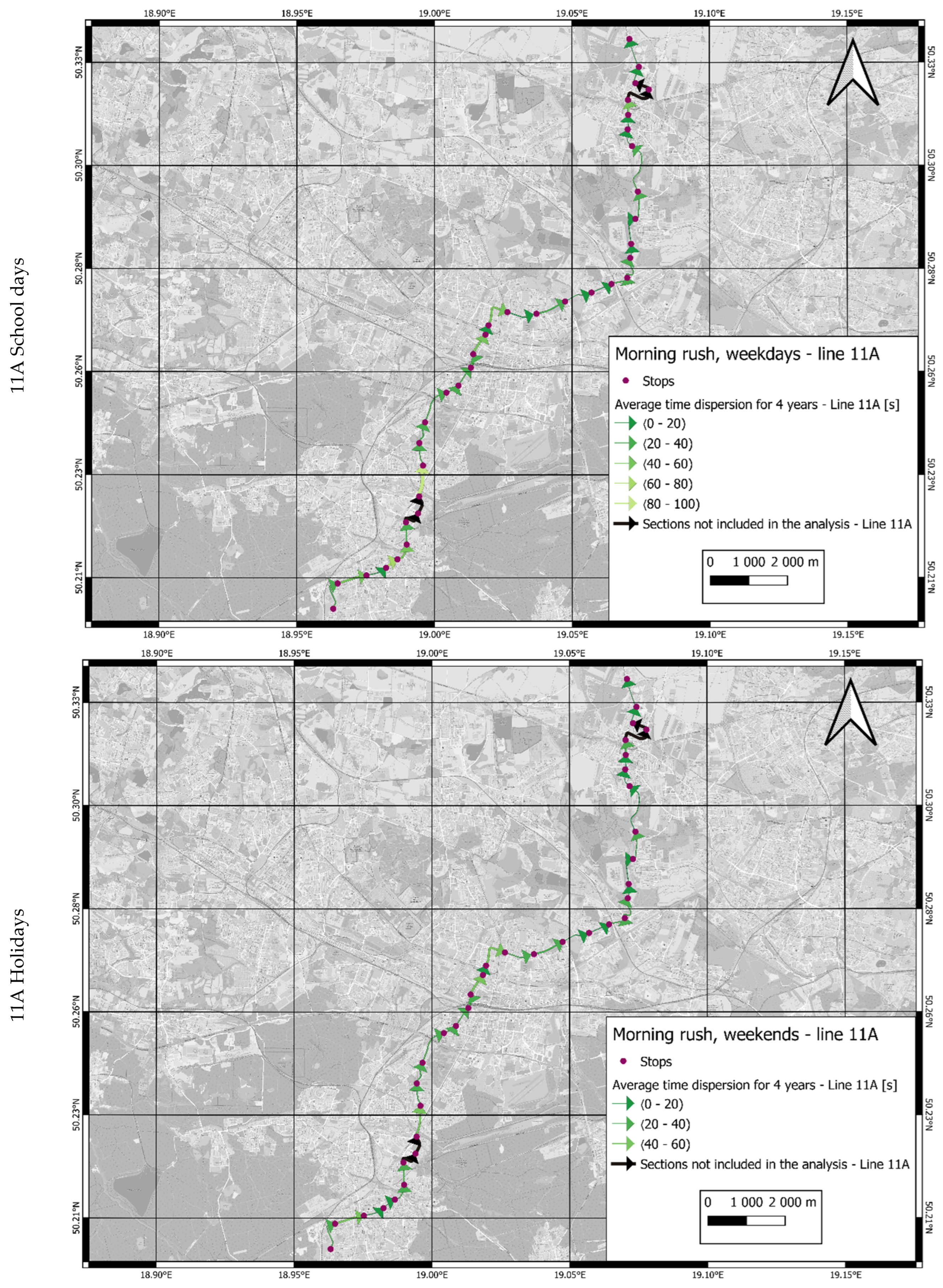
- School days morning rush hours (SM);
- -
- Holidays (all days off from school) morning rush hours (HM);
- -
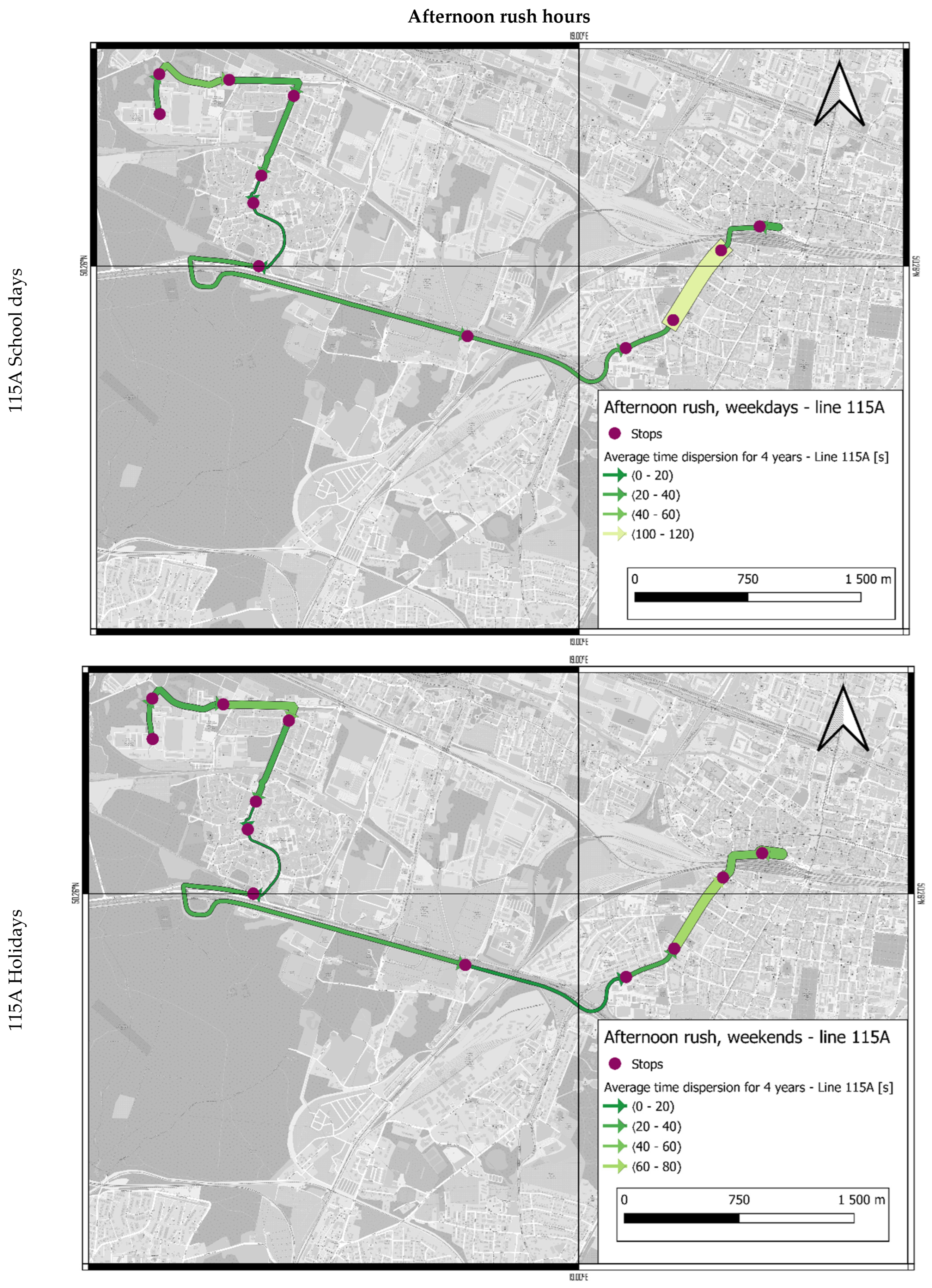
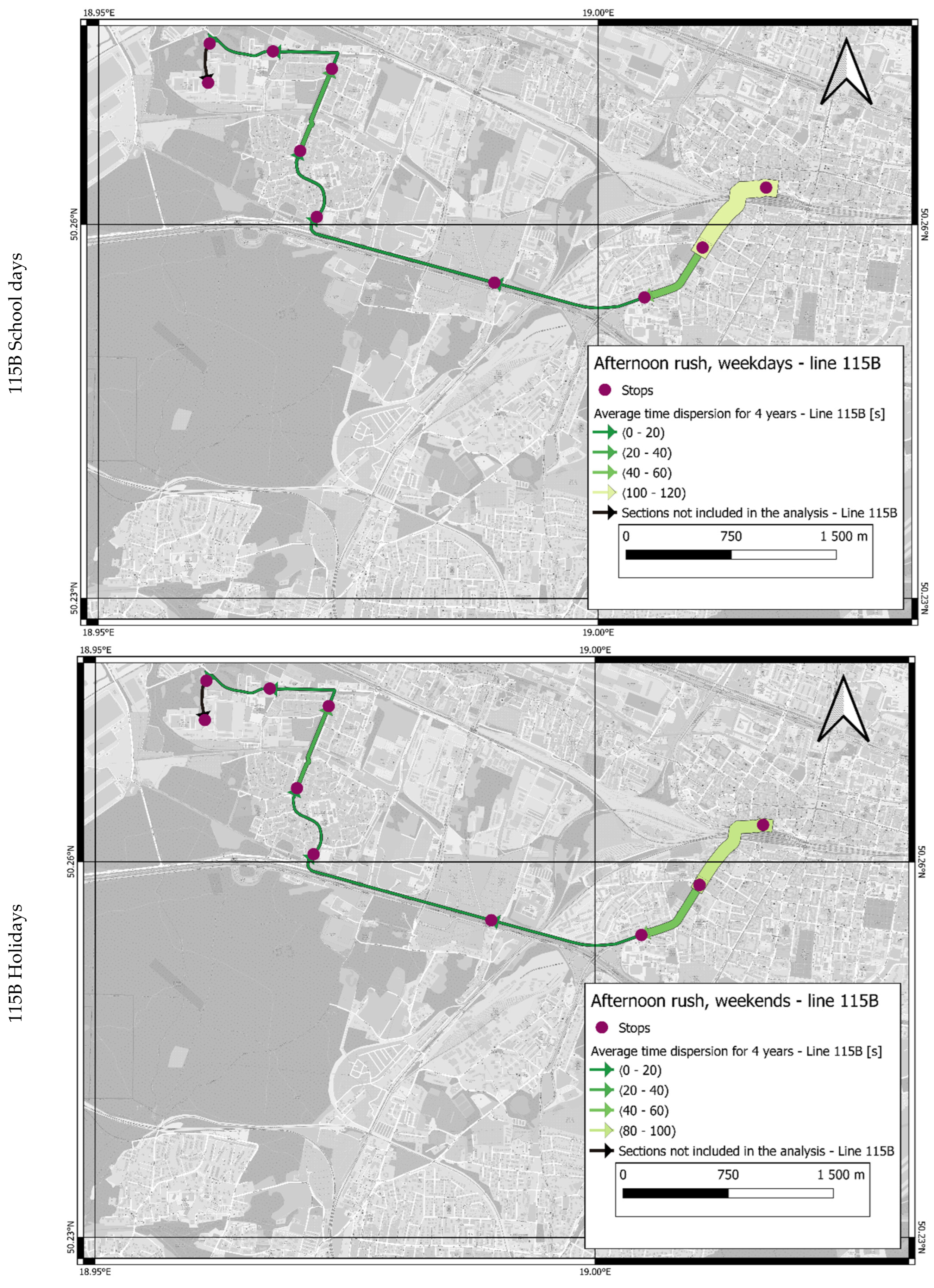
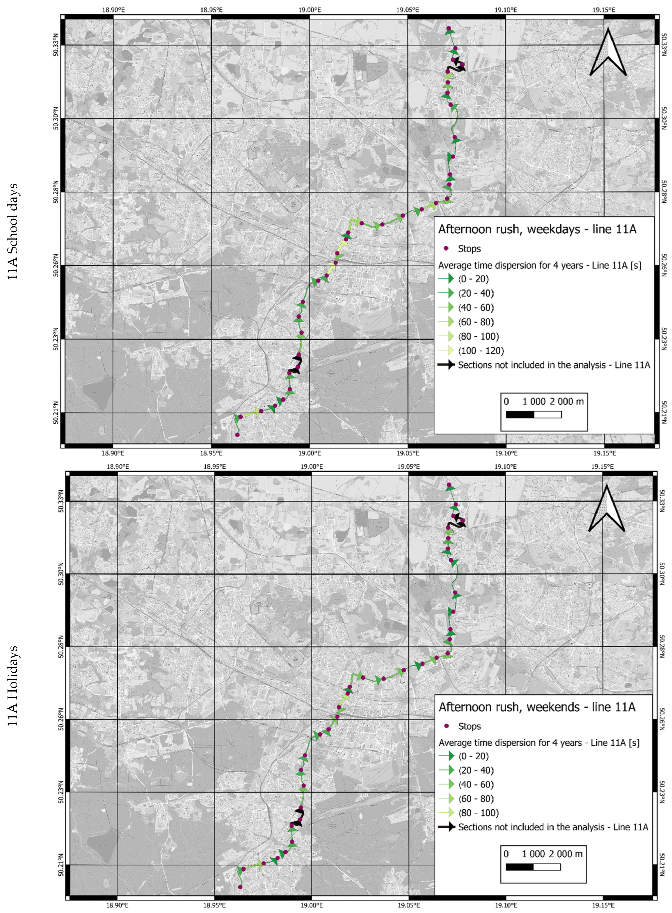
- School days afternoon rush hours (SA);
- -
- Holidays (all days off from school) afternoon rush hours (HA).
3.2. The Outline of the Method
4. Case Study
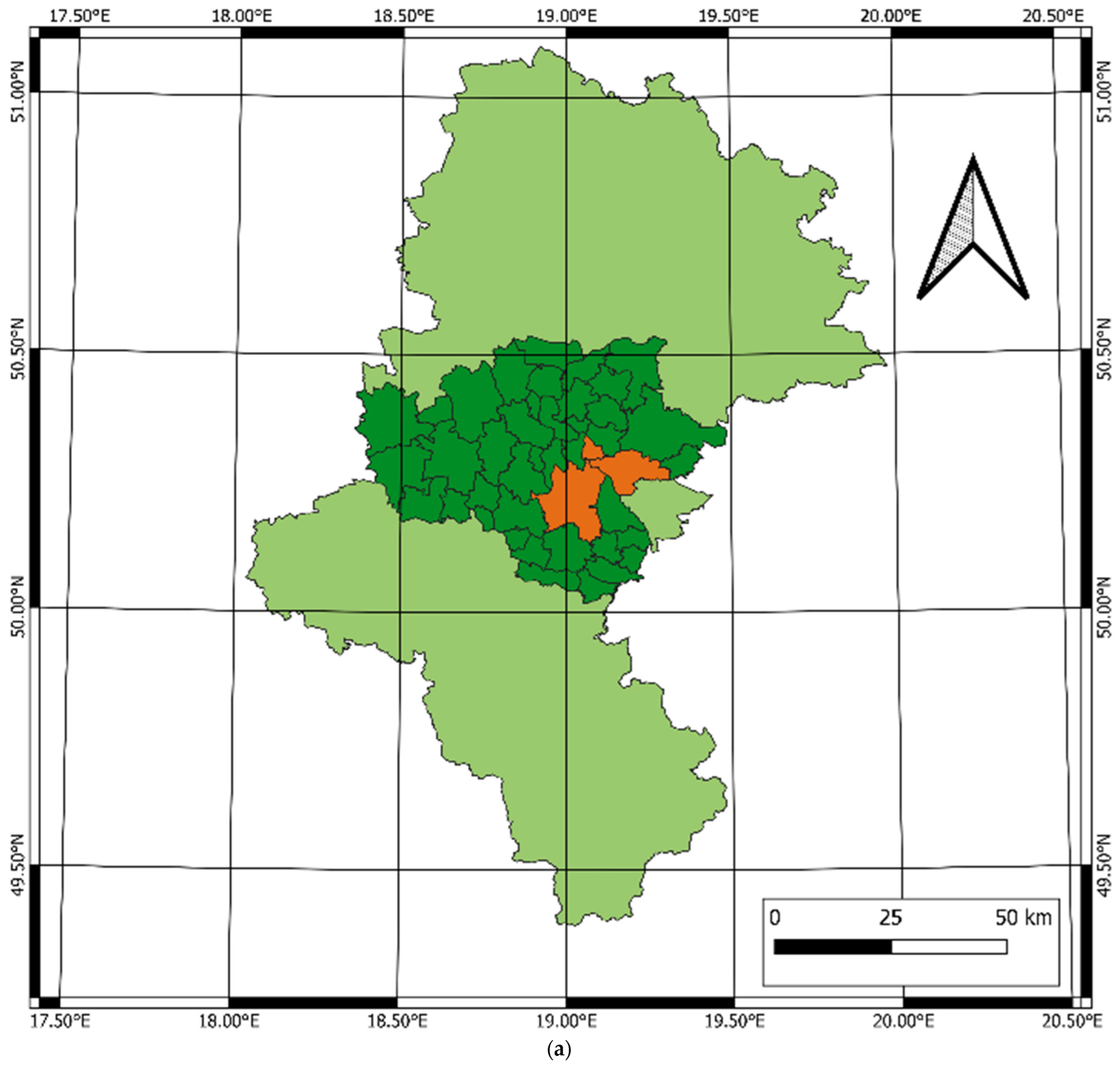
4.1. Study Area and Bus Routes
4.2. Data Filtering
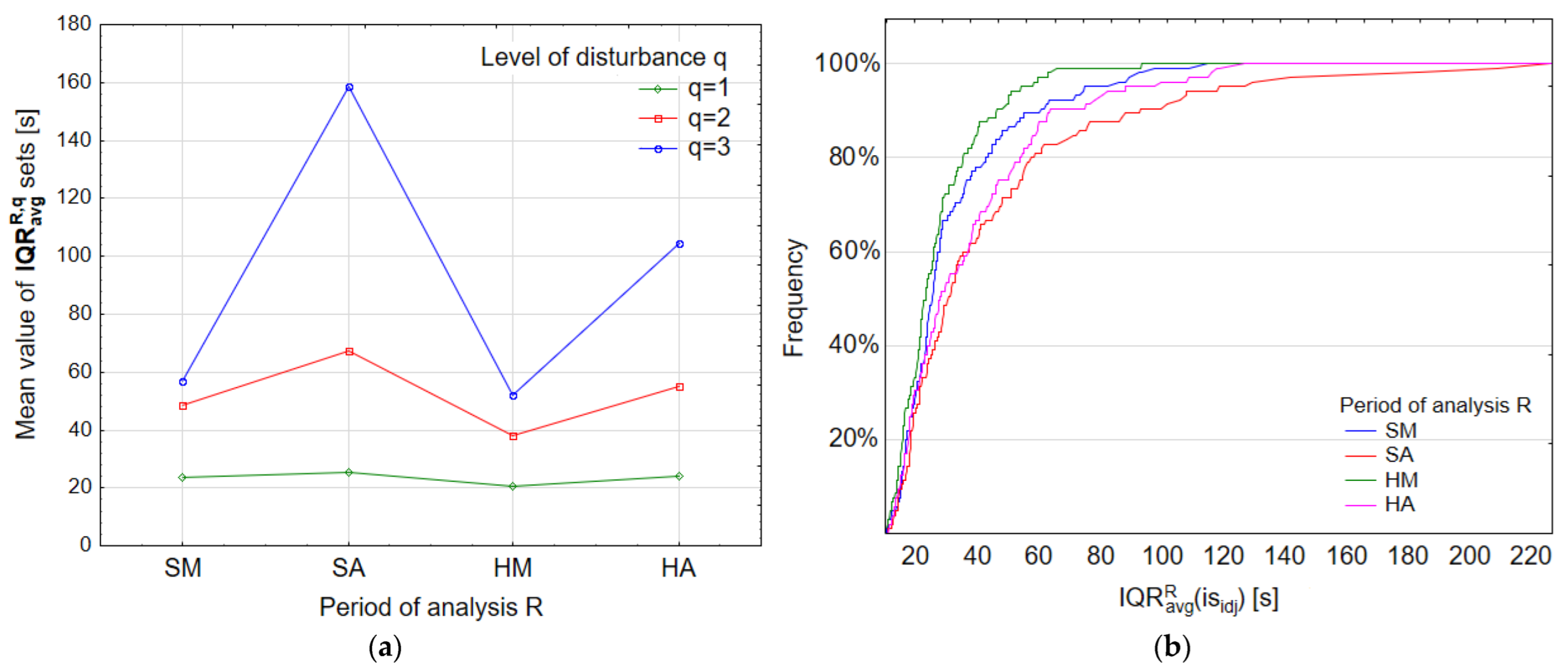
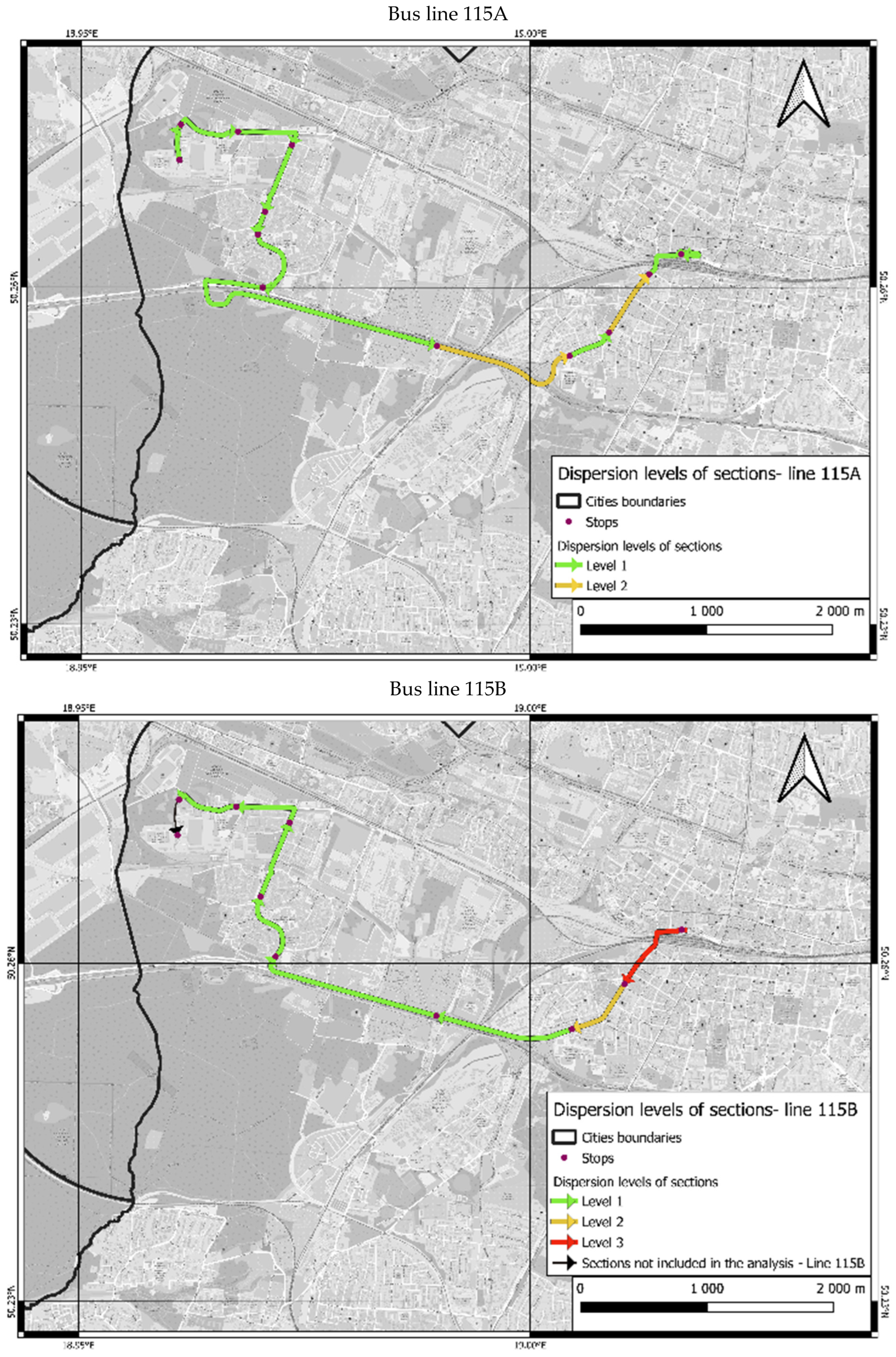
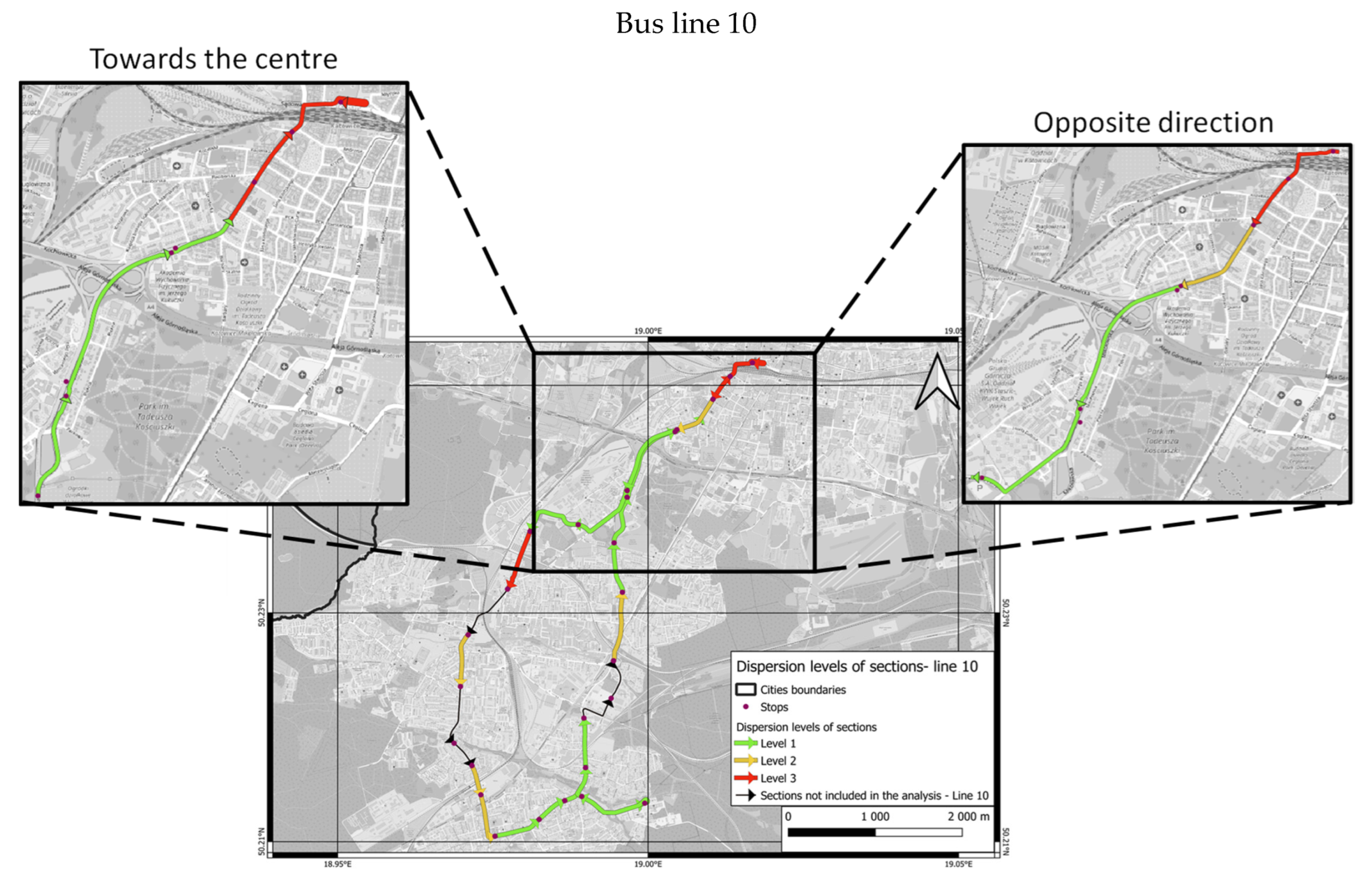
4.3. Results
5. Discussion
6. Conclusions
Author Contributions
Funding
Acknowledgments
Conflicts of Interest
Appendix A
References
- Zhang, T.; Chan, A.H.S.; Xue, H.; Zhang, X.; Tao, D. Driving Anger, Aberrant Driving Behaviors, and Road Crash Risk: Testing of a Mediated Model. Int. J. Environ. Res. Public Health 2019, 16, 297. [Google Scholar] [CrossRef] [Green Version]
- Olsson, L.E.; Friman, M. Accessibility Barriers and Perceived Accessibility: Implications for Public Transport. Urban Sci. 2021, 5, 63. [Google Scholar] [CrossRef]
- Rith, M.; Fillone, A.; Biona, J.B.M. The Impact of Socioeconomic Characteristics and Land Use Patterns on Household Vehicle Ownership and Energy Consumption in an Urban Area with Insufficient Public Transport Service–A Case Study of Metro Manila. J. Transp. Geogr. 2019, 79, 102484. [Google Scholar] [CrossRef]
- Kłos, M.J.; Sierpiński, G. Building a Model of Integration of Urban Sharing and Public Transport Services. Sustainability 2021, 13, 3086. [Google Scholar] [CrossRef]
- Jacek Kłos, M. Estimation of effects caused by the implementation of park ride system in the transport hub. Transport Problems 2016, 11, 5–12. [Google Scholar] [CrossRef]
- Sierpiński, G.; Staniek, M.; Kłos, M.J. Decision Making Support for Local Authorities Choosing the Method for Siting of In-City EV Charging Stations. Energies 2020, 13, 4682. [Google Scholar] [CrossRef]
- Jedynak, T.; Wąsowicz, K. The Relationship between Efficiency and Quality of Municipally Owned Corporations: Evidence from Local Public Transport and Waste Management in Poland. Sustainability 2021, 13, 9804. [Google Scholar] [CrossRef]
- Jacyna, M.; Wasiak, M.; Lewczuk, K.; Karoń, G. Noise and Environmental Pollution from Transport: Decisive Problems in Developing Ecologically Efficient Transport Systems. J. Vibroeng. 2017, 19, 5639–5655. [Google Scholar] [CrossRef] [Green Version]
- Chamier Gliszczyński, N. Sustainable Operation of a Transport System in Cities. Key Eng. Mater. 2011, 486, 175–178. [Google Scholar] [CrossRef]
- Bauer, M.; Bauer, K. Analysis of the Impact of the COVID-19 Pandemic on the Future of Public Transport: Example of Warsaw. Sustainability 2022, 14, 7268. [Google Scholar] [CrossRef]
- Bauer, M.; Dźwigoń, W.; Richter, M. Personal Safety of Passengers during the First Phase Covid-19 Pandemic in the Opinion of Public Transport Drivers in Krakow. Arch. Transp. 2021, 59, 41–55. [Google Scholar] [CrossRef]
- Szczepanek, W.K.; Kruszyna, M. The Impact of COVID-19 on the Choice of Transport Means in Journeys to Work Based on the Selected Example from Poland. Sustainability 2022, 14, 7619. [Google Scholar] [CrossRef]
- Cieśla, M.; Kuśnierz, S.; Modrzik, O.; Niedośpiał, S.; Sosna, P. Scenarios for the Development of Polish Passenger Transport Services in Pandemic Conditions. Sustainability 2021, 13, 10278. [Google Scholar] [CrossRef]
- Tubis, A.A.; Skupień, E.T.; Rydlewski, M. Method of Assessing Bus Stops Safety Based on Three Groups of Criteria. Sustainability 2021, 13, 8275. [Google Scholar] [CrossRef]
- Jakimavičius, K.; Palevičius, V.; Antuchevičiene, J.; Karpavičius, T. Internet GIS-Based Multimodal Public Transport Trip Planning Information System for Travelers in Lithuania. ISPRS Int. J. Geoinf. 2019, 8, 319. [Google Scholar] [CrossRef] [Green Version]
- Cascetta, E.; Cartenì, A. A Quality-Based Approach to Public Transportation Planning: Theory and a Case Study. Int. J. Sustain. Transp. 2014, 8, 84–106. [Google Scholar] [CrossRef] [Green Version]
- Krawiec, K.; Kłos, M.J. Parameters of Bus Lines Influencing the Allocation of Electric Buses to the Transport Tasks. In Scientific And Technical Conference Transport Systems Theory And Practice; Springer: Berlin/Heidelberg, Germany, 2018; pp. 129–138. [Google Scholar]
- Kaczmarczyk, M.; Sowizdzał, A.; Tomaszewska, B. Energetic and Environmental Aspects of Individual Heat Generation for Sustainable Development at a Local Scale-A Case Study from Poland. Energies 2020, 13, 454. [Google Scholar] [CrossRef] [Green Version]
- Żochowska, R.; Jacyna, M.; Kłos, M.J.; Soczówka, P. A GIS-Based Method of the Assessment of Spatial Integration of Bike-Sharing Stations. Sustainability 2021, 13, 3894. [Google Scholar] [CrossRef]
- O’Connor, D.; Caulfield, B. Level of Service and the Transit Neighbourhood-Observations from Dublin City and Suburbs. Res. Transp. Econ. 2018, 69, 59–67. [Google Scholar] [CrossRef] [Green Version]
- Sun, Y.; Wu, M.; Li, H. Using Gps Trajectories to Adaptively Plan Bus Lanes. Appl. Sci. 2021, 11, 1035. [Google Scholar] [CrossRef]
- Bok, J.; Kwon, Y. Comparable Measures of Accessibility to Public Transport Using the General Transit Feed Specification. Sustainability 2016, 8, 224. [Google Scholar] [CrossRef] [Green Version]
- Krawiec, K.; Kłos, M.J. Autonomous Bus Fleet in the Context of the Conventional-to-Electric Fleet Conversion Process. In Electric Mobility in Public Transport—Driving Towards Cleaner Air; Springer Nature: Berlin/Heidelberg, Germany, 2021; pp. 189–199. [Google Scholar]
- Zhang, Y.; Deng, J.; Zhu, K.; Tao, Y.; Liu, X.; Cui, L. Location and Expansion of Electric Bus Charging Stations Based on Gridded Affinity Propagation Clustering and a Sequential Expansion Rule. Sustainability 2021, 13, 8957. [Google Scholar] [CrossRef]
- Zoltowska, I.; Lin, J. Optimal Charging Schedule Planning for Electric Buses Using Aggregated Day-Ahead Auction Bids. Energies 2021, 14, 4727. [Google Scholar] [CrossRef]
- Połom, M.; Wiśniewski, P. Assessment of the Emission of Pollutants from Public Transport Based on the Example of Diesel Buses and Trolleybuses in Gdynia and Sopot. Int. J. Environ. Res. Public Health 2021, 18, 8379. [Google Scholar] [CrossRef] [PubMed]
- Xiaoliang, Z.; Limin, J. Analysis of Bus Line Operation Reliability Based on Copula Function. Sustainability 2021, 13, 8419. [Google Scholar] [CrossRef]
- Lin, J.; Wang, P.; Barnum, D.T. A Quality Control Framework for Bus Schedule Reliability. Transp. Res. E Logist. Transp. Rev. 2008, 44, 1086–1098. [Google Scholar] [CrossRef]
- Eboli, L.; Mazzulla, G. Performance Indicators for an Objective Measure of Public Transport Service Quality. Eur. Transp.-Trasp. Eur. 2012, 51, 1–21. [Google Scholar]
- Mishra, S.; Tang, L.; Ghader, S.; Mahapatra, S.; Zhang, L. Estimation and Valuation of Travel Time Reliability for Transportation Planning Applications. Case Stud. Transp. Policy 2018, 6, 51–62. [Google Scholar] [CrossRef]
- Durán-Hormazábal, E.; Tirachini, A. Estimation of Travel Time Variability for Cars, Buses, Metro and Door-to-Door Public Transport Trips in Santiago, Chile. Res. Transp. Econ. 2016, 59, 26–39. [Google Scholar] [CrossRef]
- Engelson, L.; Fosgerau, M. The Cost of Travel Time Variability: Three Measures with Properties. Transp. Res. Part B Methodol. 2016, 91, 555–564. [Google Scholar] [CrossRef] [Green Version]
- Jenelius, E. The Value of Travel Time Variability with Trip Chains, Flexible Scheduling and Correlated Travel Times. Transp. Res. Part B Methodol. 2012, 46, 762–780. [Google Scholar] [CrossRef]
- Sullivan, J.L.; Novak, D.C.; Aultman-Hall, L.; Scott, D.M. Identifying Critical Road Segments and Measuring System-Wide Robustness in Transportation Networks with Isolating Links: A Link-Based Capacity-Reduction Approach. Transp. Res. Part A Policy Pract. 2010, 44, 323–336. [Google Scholar] [CrossRef]
- Tampère, C.M.J.; Stada, J.; Immers, B.; Peetermans, E.; Organe, K. Methodology for Identifying Vulnerable Sections in a National Road Network. Transp. Res. Rec. 2012, 2007, 1–10. [Google Scholar] [CrossRef]
- Beaud, M.; Blayac, T.; Stéphan, M. Value of Travel Time Reliability: Two Alternative Measures. Procedia Soc. Behav. Sci. 2012, 54, 349–356. [Google Scholar] [CrossRef] [Green Version]
- Blayac, T.; Stéphan, M. Are Retrospective Rail Punctuality Indicators Useful? Evidence from Users Perceptions. Transp. Res. Part A Policy Pract. 2021, 146, 193–213. [Google Scholar] [CrossRef]
- Cats, O.; Hijner, A.M. Indicators of Spatial Passenger Delay Propagation and Their Relation to Topological Indicators. Review for INSTR2020. 2020. Available online: https://repository.tudelft.nl/islandora/object/uuid%3Ac8bbc57f-cd47-4bf1-9d9f-96c97804c24d (accessed on 4 October 2022).
- Buba, A.T.; Lee, L.S. A Differential Evolution for Simultaneous Transit Network Design and Frequency Setting Problem. Expert Syst. Appl. 2018, 106, 277–289. [Google Scholar] [CrossRef]
- Pternea, M.; Kepaptsoglou, K.; Karlaftis, M.G. Sustainable Urban Transit Network Design. Transp. Res. Part A Policy Pract. 2015, 77, 276–291. [Google Scholar] [CrossRef]
- Jara-Díaz, S.R.; Gschwender, A.; Ortega, M. Is Public Transport Based on Transfers Optimal? A Theoretical Investigation. Transp. Res. Part B Methodol. 2012, 46, 808–816. [Google Scholar] [CrossRef]
- Owais, M.; Osman, M.K. Complete Hierarchical Multi-Objective Genetic Algorithm for Transit Network Design Problem. Expert Syst. Appl. 2018, 114, 143–154. [Google Scholar] [CrossRef]
- Srinivasan, K.K.; Prakash, A.A.; Seshadri, R. Finding Most Reliable Paths on Networks with Correlated and Shifted Log-Normal Travel Times. Transp. Res. Part B Methodol. 2014, 66, 110–128. [Google Scholar] [CrossRef]
- Taylor, M.A.P.; D’Este, G.M. Transport Network Vulnerability: A Method for Diagnosis of Critical Locations in Transport Infrastructure Systems. Adv. Spat. Sci. 2007, 2, 9–30. [Google Scholar] [CrossRef]
- Yao, B.; Hu, P.; Lu, X.; Gao, J.; Zhang, M. Transit Network Design Based on Travel Time Reliability. Transp. Res. Part C Emerg. Technol. 2014, 43, 233–248. [Google Scholar] [CrossRef]
- Yu, B.; Yang, Z.Z.; Jin, P.H.; Wu, S.H.; Yao, B.Z. Transit Route Network Design-Maximizing Direct and Transfer Demand Density. Transp. Res. Part C Emerg. Technol. 2012, 22, 58–75. [Google Scholar] [CrossRef]
- van Oort, N.; van Nes, R. Regularity Analysis for Optimizing Urban Transit Network Design. Public Transp. 2009, 1, 155–168. [Google Scholar] [CrossRef]
- Farahani, R.Z.; Miandoabchi, E.; Szeto, W.Y.; Rashidi, H. A Review of Urban Transportation Network Design Problems. Eur. J. Oper. Res. 2013, 229, 281–302. [Google Scholar] [CrossRef] [Green Version]
- Cadarso, L.; Codina, E.; Escudero, L.F.; Marín, A. Rapid Transit Network Design: Considering Recovery Robustness and Risk Aversion Measures. Transp. Res. Procedia 2017, 22, 255–264. [Google Scholar] [CrossRef]
- Cancela, H.; Mauttone, A.; Urquhart, M.E. Mathematical Programming Formulations for Transit Network Design. Transp. Res. Part B Methodol. 2015, 77, 17–37. [Google Scholar] [CrossRef]
- Nicholson, A.J. Road Network Unreliability: Impact Assessment and Mitigation. Int. J. Crit. Infrastruct. 2007, 3, 346–375. [Google Scholar] [CrossRef]
- Mees, P.; Stone, J.; Imran, M.; Nielson, G. Public Transport Network Planning: A Guide to Best Practice in NZ Cities March 2010; NZ Transport Agency: Wellington, New Zealand, 2010; ISBN 9780478352917. [Google Scholar]
- Planu Zrównoważonego Rozwoju Publicznego Transportu Zbiorowego Dla Obszaru Górnośląsko-Zagłębiowskiej Metropolii Oraz Gmin, z Którymi Zawarto Porozumienie w Sprawie Powierzenia Górnośląsko-Zagłębiowskiej Metropolii Zadania Własnego Gmin, Tj. Pełnienia Funkcji Organizatora Publicznego Transportu Zbiorowego. Available online: https://bip.metropoliagzm.pl/uchwala/127154/uchwala-nr-xxxiii-262-2021 (accessed on 4 October 2022).
- Green Paper “Towards a New Culture for Urban Mobility”. Available online: https://ec.europa.eu/commission/presscorner/detail/en/MEMO_07_379 (accessed on 4 October 2022).
- STRATEGIA ROZWOJU TRANSPORTU 2020 ROKU. Available online: https://www.gov.pl/static/mi_arch/media/3511/Strategia_Rozwoju_Transportu_do_2020_roku.pdf (accessed on 4 October 2022).
- STRATEGIA ROZWOJU MIASTA Katowice 2030. Available online: https://katowice.eu/dla-mieszka%C5%84ca/strategie-i-raporty/strategia-rozwoju-miasta-2030 (accessed on 4 October 2022).


| Characteristics of Bus Lines | Direction of Bus Line | ||||
|---|---|---|---|---|---|
| 11A | 11B | 115A | 115B | 10A | |
| Number of interstop sections | 31 | 33 | 11 | 8 | 22 |
| Number of recorded departures | 164,927 | 176,992 | 92,366 | 84,231 | 107,458 |
| 2016 | 37,811 | 41,568 | 17,017 | 19,649 | 23,271 |
| School days morning rush hours SM | 13,918 | 16,091 | 6642 | 7793 | 9104 |
| School days afternoon rush hours SA | 14,036 | 14,204 | 6199 | 7204 | 7692 |
| Holidays morning rush hours HM | 4928 | 6076 | 2323 | 2567 | 3364 |
| Holidays afternoon rush hours HA | 4929 | 5197 | 1853 | 2085 | 3111 |
| 2017 | 41,518 | 43,268 | 21,309 | 21,359 | 28639 |
| School days morning rush hours SM | 15,496 | 16,723 | 8239 | 8440 | 10,975 |
| School days afternoon rush hours SA | 14,596 | 14,651 | 7762 | 7981 | 9594 |
| Holidays morning rush hours HM | 5715 | 6388 | 2867 | 2510 | 4170 |
| Holidays afternoon rush hours HA | 5711 | 5506 | 2441 | 2428 | 3900 |
| 2018 | 41,668 | 43,702 | 26,446 | 20,833 | 23,732 |
| School days morning rush hours SM | 16,687 | 18,351 | 11,109 | 8422 | 11,355 |
| School days afternoon rush hours SA | 15,971 | 15,435 | 9350 | 8064 | 10,827 |
| Holidays morning rush hours HM | 4528 | 5318 | 3311 | 2300 | 801 |
| Holidays afternoon rush hours HA | 4482 | 4598 | 2676 | 2047 | 749 |
| 2019 | 43,930 | 48,454 | 27,594 | 22,390 | 31,816 |
| School days morning rush hours SM | 16,569 | 18,772 | 10,962 | 8504 | 12,129 |
| School days afternoon rush hours SA | 16,102 | 17,240 | 9247 | 8111 | 11,135 |
| Holidays morning rush hours HM | 5706 | 6479 | 4035 | 2918 | 4379 |
| Holidays afternoon rush hours HA | 5553 | 5963 | 3350 | 2857 | 4173 |
| Level of Disturbance q | Linear and Square Euclidean Distance between Clusters | Number of Interstop Sections | ||
|---|---|---|---|---|
| 1 | 2 | 3 | ||
| 1 | - | 30.09 [s] | 80.98 [s] | 73 |
| 2 | 905.70 [s2] | - | 52.52 [s] | 25 |
| 3 | 6557.78 [s2] | 2759.01 [s2] | - | 7 |
| Period of Analysis R | Selected Measures of Summary Statistics | Level of Disturbance q | ||
|---|---|---|---|---|
| 1 | 2 | 3 | ||
| SM | Mean of | 23.4 | 48.5 | 56.8 |
| Standard deviation of | 11.4 | 23.8 | 25.0 | |
| Maximum value in | 86.0 | 114.6 | 97.4 | |
| Minimum value in | 10.4 | 16.6 | 26.6 | |
| SA | Mean of | 25.6 | 67.3 | 158.5 |
| Standard deviation of | 10.0 | 21.4 | 47.9 | |
| Maximum value in | 54.7 | 108.0 | 226.5 | |
| Minimum value in | 10.8 | 23.4 | 101.4 | |
| HM | Mean of | 20.5 | 37.9 | 52.1 |
| Standard deviation of | 7.0 | 11.9 | 23.4 | |
| Maximum value in | 50.7 | 65.9 | 93.5 | |
| Minimum value in | 10.2 | 16.0 | 26.7 | |
| HA | Mean of | 24.3 | 55.1 | 104.6 |
| Standard deviation of | 9.7 | 13.4 | 18.2 | |
| Maximum value in | 51.5 | 82.2 | 127.0 | |
| Minimum value in | 11.1 | 19.1 | 75.0 | |
| Attribute of Bus Line | Level of Disturbances q | Bus Line | ||
|---|---|---|---|---|
| 115 | 11 | 10 | ||
| Number of interstop sections allocated to level of dispersion | Level 1 | 15 | 45 | 13 |
| Level 2 | 3 | 17 | 5 | |
| Level 3 | 1 | 2 | 4 | |
| values characterising interstop sections in each level of dispersion | Level 1 | 22.29 | 22.1 | 29.39 |
| Level 2 | 46.45 | 52.77 | 53.68 | |
| Level 3 | 82.15 | 105.4 | 89.49 | |
| Total length of interstop sections allocated to level of dispersion [km] | Level 1 | 11.3 | 28.7 | 9 |
| Level 2 | 2.4 | 11.7 | 2.9 | |
| Level 3 | 0.7 | 2.3 | 2.7 | |
| value | 29.23 | 34.99 | 45.33 | |
Publisher’s Note: MDPI stays neutral with regard to jurisdictional claims in published maps and institutional affiliations. |
© 2022 by the authors. Licensee MDPI, Basel, Switzerland. This article is an open access article distributed under the terms and conditions of the Creative Commons Attribution (CC BY) license (https://creativecommons.org/licenses/by/4.0/).
Share and Cite
Barchański, A.; Żochowska, R.; Kłos, M.J. A Method for the Identification of Critical Interstop Sections in Terms of Introducing Electric Buses in Public Transport. Energies 2022, 15, 7543. https://doi.org/10.3390/en15207543
Barchański A, Żochowska R, Kłos MJ. A Method for the Identification of Critical Interstop Sections in Terms of Introducing Electric Buses in Public Transport. Energies. 2022; 15(20):7543. https://doi.org/10.3390/en15207543
Chicago/Turabian StyleBarchański, Adrian, Renata Żochowska, and Marcin Jacek Kłos. 2022. "A Method for the Identification of Critical Interstop Sections in Terms of Introducing Electric Buses in Public Transport" Energies 15, no. 20: 7543. https://doi.org/10.3390/en15207543